


1. Introduction
Nonlinear integrable equations are widely recognized for their critical role in mathematical physics and engineering, encompassing fields such as fluid mechanics, plasma physics, and ocean communications [1–4]. Nonlinear phenomena in nature can be described by nonlinear partial differential equations. In particular, high-dimensional integrable systems are more suitable for describing certain complex physical phenomena. Solving the exact and numerical solutions of integrable equations has become an important topic, attracting increasing attention from researchers [5–9]. It is noteworthy that the study of high-dimensional nonlocal integrable equations has gained widespread attention in recent years. Of particular interest is the exploration of the application of the physics informed neural network (PINN) algorithm in solving high-dimensional nonlocal integrable equations.
In this article, we are committed to solving forward and inverse problems for several integrable two-dimensional nonlocal equations via using the PINN deep learning method, focusing on the partial reverse space y-nonlocal Mel'nikov equation equation [10]
$\begin{eqnarray}\begin{array}{l}3{u}_{{yy}}-{u}_{{xt}}-\left(3{u}^{2}+{u}_{{xx}}+k{\rm{\Psi }}(x,y,t)\right.\\ \times {\left.{\rm{\Psi }}(x,-y,t)\right)}_{{xx}}=0,\\ {\rm{i}}{{\rm{\Psi }}}_{y}=u{\rm{\Psi }}+{{\rm{\Psi }}}_{{xx}},\end{array}\end{eqnarray}$
the partial reverse space-time nonlocal Mel'nikov equation [11] $\begin{eqnarray}\begin{array}{l}3{u}_{{yy}}-{u}_{{xt}}-{\left(3{u}^{2}+{u}_{{xx}}+k{\rm{\Psi }}(x,y,t){{\rm{\Psi }}}^{* }(-x,y,-t)\right)}_{{xx}}=0,\\ {\rm{i}}{{\rm{\Psi }}}_{y}=u{\rm{\Psi }}+{{\rm{\Psi }}}_{{xx}},\end{array}\end{eqnarray}$
and the nonlocal two-dimensional nonlinear Schrödinger (NLS) equation [12] $\begin{eqnarray}\begin{array}{l}{\rm{i}}{u}_{t}+{u}_{{xx}}+{u}_{{yy}}-2{u}_{{xy}}+2{uV}=0,\\ V=u(x,y,t){u}^{* }(-x,-y,t).\end{array}\end{eqnarray}$
The local Mel'nikov equation can describe the interaction between the long waves and short wave packets [13–15]. This equation can be regarded as a generalization of the Kadomtsev–Petviashvili (KP) equation by introducing a complex scalar field or as a generalization of the NLS equation by introducing a real scalar field [16–18]. For the partial reverse space y-nonlocal Mel'nikov equation, soliton and rational solutions have been obtained through the KP reduction method [10]. For the partial reverse space-time nonlocal Mel'nikov equation, solitons and breathers on periodic wave backgrounds have been constructed [19, 20]. General bright and dark soliton solutions for the partial reverse space-time nonlocal Mel'nikov equation were constructed by the Hirota bilinear method [11]. For the nonlocal two-dimensional NLS equation, it can be reduced to a (2+1)-dimensional NLS equation in the Heisenberg ferromagnetic spin chain [21–24].With the rapid development of computational power, utilizing deep learning to solve partial differential equations has garnered increasing attention from experts and scholars. Notably, Karniadakis et al recently introduced a novel neural network called PINN, which can solve partial differential equations with fewer datasets [8]. Experimental evidence has demonstrated the effectiveness of PINN in solving equations governed by mathematical physics systems. Subsequently, the use of PINN to generate data-driven solutions and discover data-driven parameters for nonlinear partial differential equations has attracted widespread attention. In the realm of integrable systems, Chen et al have constructed soliton solutions, higher-order breather waves, rogue waves, and rogue periodic waves for various types of nonlinear evolution equations driven by data, including KdV equations, NLS equations, Kaup–Newell (KN) equations, KP equations, Manakov systems, etc [25–32]. To apply the PINN algorithm to nonlocal nonlinear integrable systems, neural networks have been improved to address the data-driven positivity issue for nonlocal equations [33, 34]. Specifically, based on conservation laws, a two-stage PINN method has been used to derive some data-driven local wave solutions [35]. The Lax pairs of integrable systems were first integrated into deep neural networks for studying data-driven local wave solutions and Lax pair spectral problems [36]. Furthermore, data-driven solutions for some other equations have also been studied [37, 38]. However, to the best of our knowledge, there has been no study on local wave solutions and inverse problems involving integrable two-dimensional nonlocal equations using PINN deep learning. Therefore, in this paper, based on the PINN method, we mainly aim to present data-driven local waves and discuss the discovery of data-driven parameters for several two-dimensional nonlocal equations.
The outline of this article is structured as follows: in section 2 , we will provide a brief introduction to the PINN method. In sections 3 and 4 , we will utilize the PINN method to investigate data-driven two soliton solutions, lump solutions, and rogue wave solutions. Additionally, in section 4 , we will discuss the data-driven parameter discovery for equation (2 ) by employing the PINN method. The conclusion will be presented in the final section.
2. The PINN deep learning method
Without loss of generality, a generalized nonlocal complex (2+1)-dimensional nonlinear partial differential equation can be expressed in the following form:
$\begin{eqnarray}{\rm{i}}u{\left(x,y,t\right)}_{t}+{ \mathcal N }[u(x,y,t),\mu ]=0,\end{eqnarray}$
where μ denotes the nonlocal term of u = u(x, y, t). The variables x, y, and t belong to the intervals [X0, X1], [Y0, Y1] and [T0, T1], respectively. ${ \mathcal N }[\cdot ]$ represents a nonlinear differential operator, which is a linear combination of u, μ, and their derivatives up to the r-th order. To facilitate the separation of the real and imaginary parts of the equation, we rewrite u(x, y, t) as uR(x, y, t) + iuI(x, y, t), where uR and uI are the real and imaginary parts, respectively. Furthermore, we have μ = μR + iμI, where μR and μI are the nonlocal terms of uR and uI, respectively.Substituting u(x, y, t) = uR(x, y, t) + iuI(x, y, t) and μ = μR + iμI into equation (4 ), we obtain the following two real equations:
$\begin{eqnarray}\left\{\begin{array}{l}{\left({u}_{R}\right)}_{t}+{{ \mathcal N }}_{R}[{u}_{R},{u}_{I},{\mu }_{R},{\mu }_{I}]=0,\\ {\left({u}_{I}\right)}_{t}+{{ \mathcal N }}_{I}[{u}_{R},{u}_{I},{\mu }_{R},{\mu }_{I}]=0.\end{array}\right.\end{eqnarray}$
We approximate the solutions uR(x, y, t), uI(x, y, t), μR(x, y, t), μI(x, y, t) using neural networks as ${\hat{u}}_{R}(x,y,t;\theta )$, ${\hat{u}}_{I}(x,y,t;\theta )$, ${\hat{\mu }}_{R}(x,y,t;\theta )$, ${\hat{\mu }}_{I}(x,y,t;\theta )$, where θ represents a set of network parameters. Substituting ${\hat{u}}_{R}(x,y,t;\theta )$, ${\hat{u}}_{I}(x,y,t;\theta )$, ${\hat{\mu }}_{R}(x,y,t;\theta )$, ${\hat{\mu }}_{I}(x,y,t;\theta )$ into the above equations, we obtain the partial differential equation residuals as $\left\{\begin{array}{l}f_{A}(x, y, t ; \theta):=\frac{\partial}{\partial t} \hat{u}_{R}(x, y, t ; \theta) \\+\mathcal{N}_{R}\left[\hat{u}_{R}(x, y, t ; \theta), \hat{u}_{I}(x, y, t ; \theta), \hat{\mu}_{R}(x, y, t ; \theta), \hat{\mu}_{I}(x, y, t ; \theta)\right], \\f_{B}(x, y, t ; \theta):=\frac{\partial}{\partial t} \hat{u}_{I}(x, y, t ; \theta) \\+\mathcal{N}_{I}\left[\hat{u}_{R}(x, y, t ; \theta), \hat{u}_{I}(x, y, t ; \theta), \hat{\mu}_{R}(x, y, t ; \theta), \hat{\mu}_{I}(x, y, t ; \theta)\right] .\end{array}\right.$
Using automatic differentiation, we compute the derivatives of ${\hat{u}}_{R}(x,y,t;\theta )$, ${\hat{u}}_{I}(x,y,t;\theta )$, ${\hat{\mu }}_{R}(x,y,t;\theta )$, ${\hat{\mu }}_{I}(x,y,t;\theta )$ to obtain fA(x, y, t; θ), fB(x, y, t; θ). Subsequently, we train the deep neural networks ${\hat{u}}_{R}(x,y,t;\theta ),{\hat{u}}_{I}(x,y,t;\theta ),{\hat{\mu }}_{R}(x,y,t;\theta ),{\hat{\mu }}_{I}(x,y,t;\theta )$ and residual networks fA, fB by optimizing the network parameters. To achieve optimal training results, we use the tanh function as the activation function and initialize the weight matrices and bias vectors using the Xavier initialization method. Finally, we minimize the following loss function using the L-BFGS optimization method [39]: $\begin{eqnarray}{{Loss}}_{\theta }={{Loss}}_{{\hat{u}}_{R}}+{{Loss}}_{{\hat{u}}_{I}}+{{Loss}}_{{f}_{A}}+{{Loss}}_{{f}_{B}},\end{eqnarray}$
with $\begin{eqnarray}\left\{\begin{array}{l}{{Loss}}_{{\hat{u}}_{R}}=\displaystyle \frac{1}{{N}_{{IB}}}\displaystyle \sum _{i=1}^{{N}_{{IB}}}| {\hat{u}}_{R}({x}_{{IB}}^{i},{y}_{{IB}}^{i},{t}_{{IB}}^{i};\theta )-{u}_{R}^{i}{| }^{2},\\ {{Loss}}_{{\hat{u}}_{I}}=\displaystyle \frac{1}{{N}_{{IB}}}\displaystyle \sum _{i=1}^{{N}_{{IB}}}| {\hat{u}}_{I}({x}_{{IB}}^{i},{y}_{{IB}}^{i},{t}_{{IB}}^{i};\theta )-{u}_{I}^{i}{| }^{2},\\ {{Loss}}_{{f}_{A}}=\displaystyle \frac{1}{{N}_{f}}\displaystyle \sum _{j=1}^{{N}_{f}}| {f}_{A}({x}_{f}^{j},{y}_{f}^{j},{t}_{f}^{j}){| }^{2},\\ {{Loss}}_{{f}_{B}}=\displaystyle \frac{1}{{N}_{f}}\displaystyle \sum _{j=1}^{{N}_{f}}| {f}_{B}({x}_{f}^{j},{y}_{f}^{j},{t}_{f}^{j}){| }^{2},\end{array}\right.\end{eqnarray}$
where $\{{x}_{{IB}}^{i},{y}_{{IB}}^{i},{t}_{{IB}}^{i},{u}_{R}^{i},{u}_{I}^{i}\}{}_{i=1}^{{N}_{{IB}}}$ are the sampled initial and boundary value training data points, and $\{{x}_{f}^{j},{y}_{f}^{j},{t}_{f}^{j}\}{}_{j=1}^{{N}_{f}}$ are the collocation points sampled for fA, fB.To facilitate a clear understanding of the PINN algorithm process, we present a schematic diagram in figure 1.
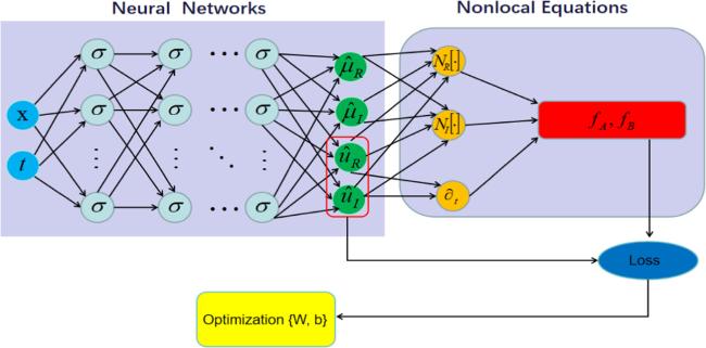
Figure 1. The PINN scheme solving the nonlocal complex (2+1)-dimensional equations. |
3. Numerical experiments for y-nonlocal Mel'nikov equation
In this section, we employ PINN to learn local wave solutions of the y-nonlocal Mel'nikov equation (1 ) with k = 1. These localized wave solutions comprise two soliton solutions and lump solutions. These solutions are derived using the KP hierarchy reduction method described in [10], and their respective dynamic behaviors are discussed therein. As stated in [10], the exact forms of these solutions can be expressed as follows:
$\begin{eqnarray}\begin{array}{rcl}u & = & \displaystyle \frac{20\sqrt{2}\cosh \tfrac{y}{2}(100{{\rm{e}}}^{\tfrac{\sqrt{2}(-15t-3x)}{2}}+{{\rm{e}}}^{\tfrac{\sqrt{2}(-5t-x)}{2}})+400{{\rm{e}}}^{\sqrt{2}(-5t-x)}}{{\left(20\sqrt{2}{{\rm{e}}}^{\tfrac{\sqrt{2}(-5t-x)}{2}}\cosh \tfrac{y}{2}+100{{\rm{e}}}^{\sqrt{2}(-5t-x)}+1\right)}^{2}},\\ {\rm{\Psi }} & = & \displaystyle \frac{100\sqrt{2}{{\rm{e}}}^{\sqrt{2}(-5t-x)}-40{\rm{i}}{{\rm{e}}}^{\tfrac{\sqrt{2}(-5t-x)}{2}}\sinh \tfrac{y}{2}+\sqrt{2}}{20\sqrt{2}{{\rm{e}}}^{\tfrac{\sqrt{2}(-5t-x)}{2}}\cosh \tfrac{y}{2}+100{{\rm{e}}}^{\sqrt{2}(-5t-x)}+1}.\end{array}\end{eqnarray}$
The exact lump solution is $\begin{eqnarray}\begin{array}{rcl}u & = & \displaystyle \frac{-196{t}^{2}+(56x-56)t-4{x}^{2}+4{y}^{2}+8x}{{\left({\left(7t-x\right)}^{2}+{y}^{2}+14t-2x+2\right)}^{2}},\\ {\rm{\Psi }} & = & \displaystyle \frac{\sqrt{2}(-{x}^{2}+(14t+2)x-4{\rm{i}}y-49{t}^{2}-{y}^{2}-14t+2)}{{x}^{2}-(14t+2)x+49{t}^{2}+{y}^{2}+14t+2}.\end{array}\end{eqnarray}$
Furthermore, to obtain data-driven soliton and lump solutions, we choose the PINN architecture consisting of 6 hidden layers with 40 neurons each.3.1. The data-driven two soliton solution
First, we take x ∈ [–15, 15], y ∈ [–15, 15] and t ∈ [–1, 1] in equation (1 ) as the boundary conditions. PINN can be utilized to obtain the two soliton solutions u, $\Psi$ given in equation (9 ).
Using MATLAB software, we discretize the x-spatial region [–15, 15] into 64 points, the y-spatial region [–15, 15] into 64 points, and the time region [–1, 1] into 32 points to acquire the raw training data. Employing the Latin hypercube sampling (LHS) method [40], we randomly choose NIB = 3000 points from the initial boundary data and designate Nf = 20000 points as collocation points within the interior region. By processing this filtered training data through PINN, we successfully learn the data-driven two soliton wave solutions u(x, y, t), $\Psi$(x, y, t). The ${{\mathbb{L}}}_{2}$-norm error of the learned solutions compared to the exact solutions are 7.448 063e-04 and 3.615 855e-03. The overall learning process involves 1265 iterations and takes approximately 329.9863 seconds. The corresponding three-dimensional plots of data-driven two soliton wave solutions u(x, y, t) and $\Psi$(x, y, t) are displayed in figure 2, respectively.

Figure 2. Solving the data-driven two soliton wave solution u(x, y, t) (see (a), (b), (c)), $\Psi$(x, y, t) (see (d), (e), (f)) in the (x, y) plane for y-nonlocal Mel'nikov equation ( |
3.2. The data-driven lump wave solution
For the data-driven lump solution, we consider x ∈ [ − 6, 6], y ∈ [ − 6, 6] and t ∈ [ − 0.5, 0.5] as boundaries and obtain the corresponding initial boundary conditions from equation (10 ). Considering the discretization of (x, y, t) into 64 points, 64 points, and 32 points respectively, and randomly selecting NIB = 3000 boundary data and Nf = 20000 collocation points, we successfully generate the data-driven lump solution. Experimental results indicate ${{\mathbb{L}}}_{2}$-norm errors between the learned solution and the exact solution of 1.023 086e-03 and 1.779 104e-03 respectively. The entire learning process involves 8820 iterations and takes 2301.3082 seconds. The dynamic behavior of the data-driven lump solution is illustrated in figure 3. From figure 3, we can also observe the excellent learning performance.

Figure 3. Solving the data-driven lump wave solution u(x, y, t) (see (a), (b), (c)), $\Psi$(x, y, t) (see (d), (e), (f)) in the (x, y) plane for y-nonlocal Mel'nikov equation ( |
4. Numerical experiments for two-dimensional nonlocal NLS equation
The two-dimensional nonlocal NLS equation along with Dirichlet boundary conditions is [12]
$\left\{\begin{array}{l}\mathrm{i} u_{t}+u_{x x}+u_{y y}-2 u_{x y}+2 u V=0, V=u(x, y, t) u^{*}(-x,-y, t), \\x \in[-3,3], \quad y \in[-3,3], \quad t \in[-0.2,0.2], \\u(x,-0.2)=\mathrm{e}^{-0.4 \mathrm{i}}\left(1-\frac{1-0.8 \mathrm{i}}{(x+2 y)^{2}+0.41}\right), \\u(-3, y, t)=\mathrm{e}^{2 \mathrm{it}}\left(1-\frac{4 \mathrm{i} t+1}{4 t^{2}+(-3+2 y)^{2}+\frac{1}{4}}\right), \\u(3, y, t)=\mathrm{e}^{2 \mathrm{it}}\left(1-\frac{4 \mathrm{i} t+1}{4 t^{2}+(3+2 y)^{2}+\frac{1}{4}}\right), \\u(x,-3, t)=\mathrm{e}^{2 \mathrm{it}}\left(1-\frac{4 \mathrm{i} t+1}{4 t^{2}+(x-6)^{2}+\frac{1}{4}}\right), \\u(x, 3, t)=\mathrm{e}^{2 \mathrm{it}}\left(1-\frac{4 \mathrm{i} t+1}{4 t^{2}+(x+6)^{2}+\frac{1}{4}}\right) .\end{array}\right.$
Our objective is to employ PINN to learn the rogue wave solution u(x, y, t), which has an analytical form given by $u(x,y,t)={{\rm{e}}}^{2{\rm{i}}t}\left(1-\displaystyle \frac{4{\rm{i}}t+1}{4{t}^{2}+{\left(x+2y\right)}^{2}+\tfrac{1}{4}}\right)$. We utilize a fully connected neural network with 6 layers, each containing 40 neurons, and employ hyperbolic tangent (tanh) activation functions. In MATLAB, we discretize the analytical solution in the spatial domain [−3, 3] into 64 points and in the time domain [−0.2, 0.2] into 32 points to generate initial training data. The raw training data consists of boundary value data and interior points. From the original boundary data, we randomly select NIB = 3000 initial boundary data points and designate Nf = 20000 points as collocation points within the interior. Using this training data with the PINN approach, the data-driven rogue wave solution u(x, y, t) is learned with an ${{\mathbb{L}}}_{2}$-norm error relative to the exact solution of 2.598 890e-04. The entire learning process involves 6905 iterations and takes approximately 727.4275 seconds. The corresponding dynamic behavior is described in figure 4, which displays the wave propagation pattern in the (x, y) plane.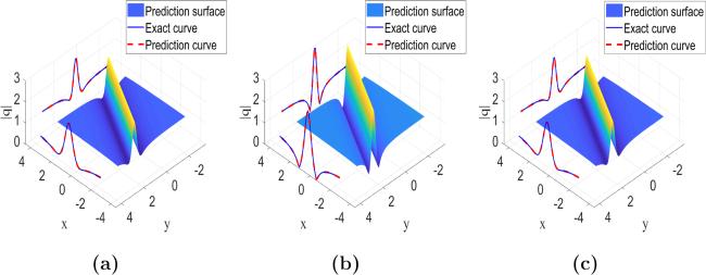
Figure 4. Solving the data-driven rogue wave solution u(x, y, t) in the (x, y) plane for two-dimensional nonlocal equation ( |
5. Numerical experiments for inverse problem
In this section, we focus on using the PINN method to solve inverse problems related to high-dimensional nonlocal equations. Specifically, we explore the partial reverse space-time nonlocal Mel'nikov equation. The reverse space-time nonlocal Mel'nikov equation with parameters can be written as:12 ). The specific solution is given as follows [11]
$\begin{eqnarray}\begin{array}{l}3{u}_{{yy}}-{u}_{{xt}}-\left(3{u}^{2}+{u}_{{xx}}+k{\rm{\Psi }}(x,y,t)\right.\\ \quad {\left.{{\rm{\Psi }}}^{* }(-x,y,-t)\right)}_{{xx}}=0,\\ {\rm{i}}{{\rm{\Psi }}}_{y}=u{\rm{\Psi }}+{{\rm{\Psi }}}_{{xx}},\quad x\in [-8,8],\\ \quad y\in [-8,8],\quad t\in [-4,4].\end{array}\end{eqnarray}$
Here, we set k = 1 to demonstrate the ability of the PINN method in learning the parameter k and the corresponding soliton solution of equation ( $\begin{eqnarray}u(x,y,t)=\displaystyle \frac{8{{\rm{e}}}^{2x-6t}}{{\left({{\rm{e}}}^{2x-8t}+{{\rm{e}}}^{2t}\right)}^{2}},\end{eqnarray}$
$\begin{eqnarray}{\rm{\Psi }}(x,y,t)=\displaystyle \frac{2\sqrt{2}{{\rm{e}}}^{x-{\rm{i}}y-3t}}{{{\rm{e}}}^{2x-8t}+{{\rm{e}}}^{2t}}.\end{eqnarray}$
Using the exact soliton wave solution (13 ) and discretizing the x-spatial region [−8, 8] into 64 points, the y-spatial region [−8, 8] into 64 points, and the time region [−4, 4] into 32 points, we can obtain a discrete dataset. By applying Latin Hypercube Sampling, we randomly select NIB = 5000 points as boundary data and Nf = 5000 points as collocation points to generate a training dataset. Using the obtained training dataset, we employ a 6-layer neural network with 40 neurons in each layer to predict the solutions u(x, y, t), $\Psi$(x, y, t), and the unknown parameter k. In the absence of noise, the ${{\mathbb{L}}}_{2}$-norm errors of the data-driven solutions u(x, y, t), $\Psi$(x, y, t) compared to the exact solutions are 1.877 311e-03 and 8.999 751e-04, respectively. Figure 5 clearly shows the 3D contour plots and 2D cross-sectional views of the data-driven soliton wave solutions in the (x, y) plane. Table 1 presents the exact parameters of the reverse space-time nonlocal Mel'nikov equation and the parameters k learned using PINN under different noise levels, along with their error rates. As seen in table 1, PINN demonstrates an excellent capability in accurately identifying the unknown parameter, especially when the training data is noise-free. Even with a noise level of 0.1, the error associated with the parameter k remains within an acceptable range, indicating robust predictions. However, as the noise level increases, the parameter error values become larger.
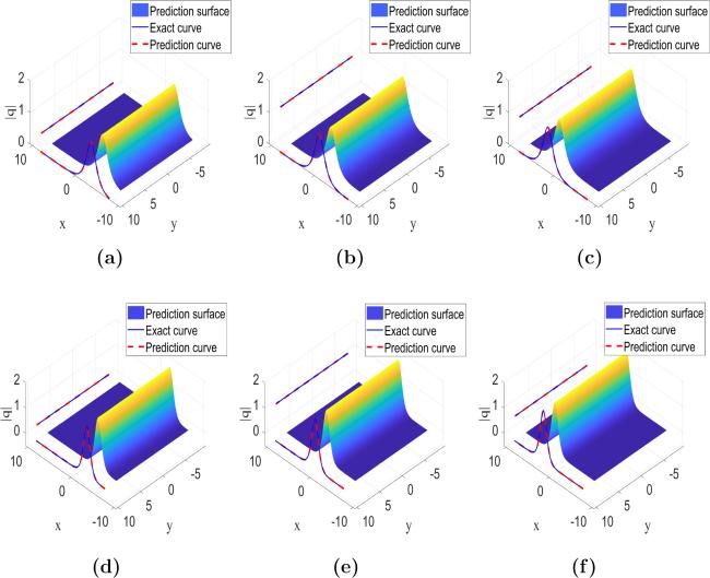
Figure 5. Solving the data-driven soliton wave solution u(x, y, t) (see (a), (b), (c)), $\Psi$(x, y, t) (see (d), (e), (f)) in the (x, y) plane for reverse space-time nonlocal Mel'nikov equation ( |
Table 1. Data-driven parameter discovery of k |
| Parameter | ||
|---|---|---|
| Noise | k | error of k |
| Correct parameter | 1 | 0 |
| Without noise | 1.000933 | 0.093 28% |
| With a 0.1 noise | 0.9913218 | 0.86782% |
| With a 0.5 noise | 0.9681684 | 3.18316% |
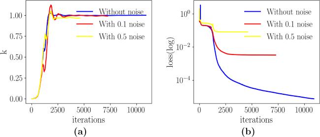
Further, we examined the variation of unknown parameters and loss functions with the number of iterations under different levels of noise. Figure 6(a) illustrates the variation of unknown parameters during the iterations under different noise conditions. It can be observed from the figure that as the noise increases, the curve gradually deviates from the curve of the true values. Figure 6(b) demonstrates the fluctuation of the loss function with the increase of iterations under different noise levels. The research results indicate that as the noise level rises, the convergence effect gradually weakens.
Figure 6. (a) The variation of unknown parameters k. (b) The variation of loss function with the different noise. |
6. Conclusion
In conclusion, we investigated data-driven local solutions and inverse problems for two-dimensional nonlocal equations using the PINN method. The PINN deep learning approach was employed to generate data-driven soliton solutions, lump solutions for the partial y-nonlocal Mel'nikov equation, and rogue wave solutions for the nonlocal two-dimensional NLS equation. It is noteworthy that obtaining data-driven solutions is quite challenging due to the increased dimensionality and the presence of nonlocal terms. This indicates that the dimensionality of the equations significantly impacts the performance of the PINN method. Additionally, we applied the PINN method to discuss data-driven parameter discovery for soliton solutions of the space-time nonlocal Mel'nikov equation. Our results demonstrate that the PINN deep learning method is highly effective and robust in studying local waves in high-dimensional nonlocal integrable systems.