Welcome to visit Communications in Theoretical Physics,
Mathematical Physics

On Sawada-Kotera and Kaup-Kuperschmidt integrable systems

  • Metin Gürses , 1 ,
  • Aslı Pekcan , 2, *
Expand
  • 1Department of Mathematics, Faculty of Science Bilkent University, 06800 Ankara, Turkey
  • 2Department of Mathematics, Faculty of Science Hacettepe University, 06800 Ankara, Turkey

*Author to whom any correspondence should be addressed.

Received date: 2024-04-05

  Revised date: 2024-08-05

  Accepted date: 2024-08-15

  Online published: 2024-11-15

Copyright

© 2024 Institute of Theoretical Physics CAS, Chinese Physical Society and IOP Publishing. All rights, including for text and data mining, AI training, and similar technologies, are reserved.

Abstract

To obtain new integrable nonlinear differential equations there are some well-known methods such as Lax equations with different Lax representations. There are also some other methods that are based on integrable scalar nonlinear partial differential equations. We show that some systems of integrable equations published recently are the ${{ \mathcal M }}_{2}$-extension of integrable such scalar equations. For illustration, we give Korteweg–de Vries, Kaup-Kupershmidt, and Sawada-Kotera equations as examples. By the use of such an extension of integrable scalar equations, we obtain some new integrable systems with recursion operators. We also give the soliton solutions of the systems and integrable standard nonlocal and shifted nonlocal reductions of these systems.

Cite this article

Metin Gürses , Aslı Pekcan . On Sawada-Kotera and Kaup-Kuperschmidt integrable systems[J]. Communications in Theoretical Physics, 2025 , 77(2) : 025003 . DOI: 10.1088/1572-9494/ad6f8e

1. Introduction

There are many ways of obtaining new integrable systems of equations such as taking the Lax representations in algebras of higher rank. In these methods we obtain real and complex valued coupled nonlinear equations which possess recursion operators and Hirota bilinear forms. There are also some other methods that use integrable systems with less number of dynamical variables to produce integrable systems with more dynamical variables. Recently, we observed such an effort to obtain systems of Sawada-Kotera (SK) and Kaup-Kuperschmidt (KK) equations [1, 2] by the use of Lax representations. The purpose of this paper is to show that the systems obtained in [1, 2] are easily obtained by a method that we call ${{ \mathcal M }}_{2}$-extensions of the SK and KK equations. This method is so general that it can be used for any integrable scalar equation.
Let ${{ \mathcal M }}_{2}$ be a special subclass of 2 × 2 matrices. Let $A\in {{ \mathcal M }}_{2}$ and be given by A = a1 I + a2 Σ where a1 and a2 are independent components of the matrix A, I is the 2 × 2 identity matrix, and
$\begin{eqnarray}{\rm{\Sigma }}=\left(\begin{array}{ll}0 & \sigma \\ 1 & 0\end{array}\right),\end{eqnarray}$
where σ is a real constant. Since Σ2 = σ I, products of all such matrices are also in this subclass of matrices. Hence ${{ \mathcal M }}_{2}$ is a commutative subclass of 2 × 2 matrices. Due to the special properties of this subclass ${{ \mathcal M }}_{2}$ of 2 × 2 matrices we can generate new systems of integrable equations from scalar integrable equations. We call this method the ${{ \mathcal M }}_{2}$-extension of integrable scalar equations. As an illustration consider the well-known Korteweg–de Vries (KdV) equation ut = uxxx + 6uux with Lax pair L = D2 + u, ${ \mathcal A }=4{D}^{3}+6{uD}+3{u}_{x}$ so that the Lax equation is satisfied by virtue of the KdV equation
$\begin{eqnarray}{L}_{t}+[L,{ \mathcal A }]=0,\end{eqnarray}$
and the recursion operator ${{ \mathcal R }}_{{KdV}}={D}^{2}+4u+2{u}_{x}{D}^{-1}$ [3]. Here D is the total x-derivative and D−1 = ∫x is the standard anti-derivative. Then ${{ \mathcal M }}_{2}$-extension of the KdV equation, its Lax pair, and recursion operator are, respectively, given as
$\begin{eqnarray}{U}_{t}={U}_{{xxx}}+6{{UU}}_{x},\end{eqnarray}$
$\begin{eqnarray}L={{ID}}^{2}+U,\end{eqnarray}$
$\begin{eqnarray}{ \mathcal A }=4{{ID}}^{3}+6{UD}+3{U}_{x},\end{eqnarray}$
$\begin{eqnarray}{ \mathcal R }={{ID}}^{2}+4U+2{U}_{x}\,{D}^{-1},\end{eqnarray}$
where
$\begin{eqnarray}U={uI}+v{\rm{\Sigma }}=\left(\begin{array}{ll}u & \sigma v\\ v & u\end{array}\right).\end{eqnarray}$
The pair L and ${ \mathcal A }$ solves the Lax equation due to the ${{ \mathcal M }}_{2}$-extension of the KdV equation (1.3) for U. In componentwise the above equations give a system of equations for the dynamical variables u and v
$\begin{eqnarray}{u}_{t}={u}_{{xxx}}+6({{uu}}_{x}+\sigma {{vv}}_{x}),\end{eqnarray}$
$\begin{eqnarray}{v}_{t}={v}_{{xxx}}+6{\left({uv}\right)}_{x},\end{eqnarray}$
admitting the recursion operator
$\begin{eqnarray}{ \mathcal R }=\left(\begin{array}{ll}{R}_{{\rm{KdV}}} & \,\sigma (4v+2{v}_{x}\,{D}^{-1})\\ 4v+2{v}_{x}\,{D}^{-1} & {R}_{{\rm{KdV}}}\end{array}\right).\end{eqnarray}$
It is interesting that the above extension of the KdV equation is equivalent to the pseudo-complexification of the KdV equation. First let σ = εσ∣ where ε = 0, ± 1. Then scale $v\to \tfrac{v}{\sqrt{| \sigma | }}$ (for σ ≠ 0) so the above system becomes
$\begin{eqnarray}{u}_{t}={u}_{{xxx}}+6({{uu}}_{x}+\epsilon {{vv}}_{x}),\end{eqnarray}$
$\begin{eqnarray}{v}_{t}={v}_{{xxx}}+6{\left({uv}\right)}_{x}.\end{eqnarray}$

For $\epsilon =0$ the above system is the extension of the KdV with its linearized equation for $v=\delta u$ (see [4]). For $\epsilon \ne 0$ this system is a consequence of the pseudo-complexification $u\to U=u+{ev}$ of the KdV equation where e is the pseudo-complex unit ${e}^{2}=\epsilon $. For complex numbers $\epsilon =-1$ but for pseudo-complex numbers $\epsilon =1$. Complex conjugation for both cases is the same ${e}^{* }=-e$. Hence our conclusion is that the ${{ \mathcal M }}_{2}$-extension of the KdV equation is the unification of linearization, complexification, and pseudo-complexification of the KdV equation. Our second conclusion is that this is valid in general.

We note that it is possible to define a second ${{ \mathcal M }}_{2}$-algebra by using a different unit Σ such that Σ2 = σ Σ, where σ is any real number. In this way we follow our approach to the KdV equation, for instance, we obtain different integrable coupled equations. Let uU = uI + vΣ then we obtain the following integrable coupled equations [5, 6]
$\begin{eqnarray}{u}_{t}={u}_{{xxx}}+6{{uu}}_{x},\end{eqnarray}$
$\begin{eqnarray}{v}_{t}={v}_{{xxx}}+6{\left({uv}\right)}_{x}+6\sigma \,{{vv}}_{x}.\end{eqnarray}$
An example of such unit is given as ${\rm{\Sigma }}=\left(\begin{array}{cc}0 & 0\\ 1 & \sigma \end{array}\right).$ One can obtain the Lax pair and the recursion operator of the above system by letting U = uI + vΣ in (1.4)–(1.6). We shall consider these two ${{ \mathcal M }}_{2}$-algebras in more detail in a forthcoming work [7]. In the rest of this work we use only the first ${{ \mathcal M }}_{2}$-algebra.
We use the ${{ \mathcal M }}_{2}$-extension method on integrable scalar equations to obtain systems of integrable equations and new integrable nonlocal equations. This method consists of three main steps. The first step is to replace the dynamical variable of the integrable scalar equation by uI + vΣ where u and v are the dynamical variables of the system. Here, since Σ2 = σI the system of equations contains also the constant σ. We write the dynamical equations for u and v. By using the recursion operator of the scalar equation we obtain the recursion operator of the system for u and v. Furthermore, if the Hirota bilinear form of the scalar equation is known then we obtain the bilinear form of the system of equations. At this step we obtain an integrable system for u and v. The second step is to obtain the symmetrical version of the system by defining new dynamical variables q = u + v and r = uv. At the same time one can obtain the recursion operator with respect to the dynamical variables q and r. The third step is to apply consistent reductions; standard (unshifted) nonlocal reductions r(x, t) = q(ε1x, ε2t) and $r(x,t)=\bar{q}({\epsilon }_{1}x,{\epsilon }_{2}t)$, and shifted nonlocal reductions r(x, t) = q(ε1x + x0, ε2t + t0) and $r(x,t)=\bar{q}({\epsilon }_{1}x+{x}_{0},{\epsilon }_{2}t+{t}_{0})$ for ${x}_{0},{t}_{0}\in {\mathbb{R}}$ where ${\epsilon }_{1}^{2}={\epsilon }_{2}^{2}=1$ to obtain standard nonlocal and shifted nonlocal reductions of the system for q and r [820]. All these equations are new and integrable. Using the reduction formulas, we can obtain the recursion operators of the nonlocal differential equations. Soliton solutions of the standard nonlocal and shifted nonlocal equations can be easily obtained by using soliton solutions of the systems and reduction formulas.

In 2 × 2 matrix algebra we have two subalgebras effective in our approach. It is possible to study the extension of the scalar integrable equations by using subalgebras of higher dimensional matrix algebras. We shall consider such extensions in later communications.

In the following section, we find ${{ \mathcal M }}_{2}$-extensions of the SK and KK equations, their recursion operators, and symmetrical versions of these systems. In section 3 we obtain nonlocal reductions of the SK and KK systems. In section 4 we find shifted nonlocal reductions of SK and KK systems. In section 5 we present Hirota bilinearization of SK and KK systems and give one-soliton solutions of these systems.

2. SK and KK systems

Recently, we observed some publications on the extensions of higher-order integrable equations by using the Lax representations [1, 2]. Here we show that such extensions are nothing but the ${{ \mathcal M }}_{2}$-extension of an integrable scalar equation explained in the previous section.
Scalar versions of SK and KK equations are given, respectively, as [1, 2, 2126]:
(1) SK equation, Lax pair and recursion operator
$\begin{eqnarray}{u}_{t}+{u}_{5x}+5{{uu}}_{{xxx}}+5{u}_{x}{u}_{{xx}}+5{u}^{2}{u}_{x}=0,\end{eqnarray}$
$\begin{eqnarray}L={D}^{3}+{uD},\end{eqnarray}$
$\begin{eqnarray}{ \mathcal A }=9{D}^{5}+15{{uD}}^{3}+15{u}_{x}{D}^{2}+5({u}^{2}+2{u}_{{xx}})D,\end{eqnarray}$
$\begin{eqnarray}\begin{array}{l}{{ \mathcal R }}_{{SK}}={D}^{6}+6{{uD}}^{4}+9{u}_{x}{D}^{3}\\ +\,(9{u}^{2}+11{u}_{{xx}}){D}^{2}+(10{u}_{{xxx}}+21{{uu}}_{x})D\\ +\,4{u}^{3}+16{{uu}}_{{xx}}+6{u}_{x}^{2}+5{u}_{4x}\\ +\,{u}_{x}{D}^{-1}(2{u}_{{xx}}+{u}^{2})-{u}_{t}\,{D}^{-1}.\end{array}\end{eqnarray}$
(2) KK equation, Lax pair and recursion operator
$\begin{eqnarray}{u}_{t}+{u}_{5x}+10{{uu}}_{{xxx}}+25{u}_{x}{u}_{{xx}}+20{u}^{2}{u}_{x}=0,\end{eqnarray}$
$\begin{eqnarray}L={D}^{3}+2{uD}+{u}_{x},\end{eqnarray}$
$\begin{eqnarray}\begin{array}{l}{ \mathcal A }=9{D}^{5}+3{{uD}}^{3}+45{u}_{x}{D}^{2}\\ +\,(20{u}^{2}+35{u}_{{xx}})D+10({u}^{2}+{u}_{{xx}}),\end{array}\end{eqnarray}$
$\begin{eqnarray}\begin{array}{l}{{ \mathcal R }}_{{KK}}={D}^{6}+12{{uD}}^{4}+36{u}_{x}{D}^{3}\\ +\,(36{u}^{2}+49{u}_{{xx}}){D}^{2}+(35{u}_{{xxx}}+120{{uu}}_{x})D\\ +\,32{u}^{3}+82{{uu}}_{{xx}}+69{u}_{x}^{2}+13{u}_{4x}\\ +\,2{u}_{x}{D}^{-1}({u}_{{xx}}+4{u}^{2})-2{u}_{t}\,{D}^{-1}.\end{array}\end{eqnarray}$
${{ \mathcal M }}_{2}$-extensions of these equations, Lax pairs and recursion operators are, respectively, given as
(3) SK system, Lax pair and recursion operator
$\begin{eqnarray}{U}_{t}+{U}_{5x}+5{{UU}}_{{xxx}}+5{U}_{x}{U}_{{xx}}+5{U}^{2}{U}_{x}=0,\end{eqnarray}$
$\begin{eqnarray}L={{ID}}^{3}+{UD},\end{eqnarray}$
$\begin{eqnarray}{ \mathcal A }=9{{ID}}^{5}+15{{UD}}^{3}+15{U}_{x}{D}^{2}+5({U}^{2}+2{U}_{{xx}})D,\end{eqnarray}$
$\begin{eqnarray}\begin{array}{l}{ \mathcal R }={{ID}}^{6}+6{{UD}}^{4}+9{U}_{x}{D}^{3}\\ +\,(9{U}^{2}+11{U}_{{xx}}){D}^{2}+(10{U}_{{xxx}}+21{{UU}}_{x})D\\ +\,4{U}^{3}+16{{UU}}_{{xx}}+6{U}_{x}^{2}+5{U}_{4x}\\ +\,{U}_{x}{D}^{-1}(2{U}_{{xx}}+{U}^{2})-{U}_{t}\,{D}^{-1}.\end{array}\end{eqnarray}$
The above equations correspond to the system of equations for the dynamical variables u and v as
$\begin{eqnarray}\begin{array}{l}{u}_{t}+{u}_{5x}+5{{uu}}_{{xxx}}+5{u}_{x}{u}_{{xx}}\\ +\,5{u}^{2}{u}_{x}+5\sigma {\left({{vv}}_{{xx}}+{v}^{2}u\right)}_{x}=0,\end{array}\end{eqnarray}$
$\begin{eqnarray}{v}_{t}+{v}_{5x}+5{\left({{vu}}_{{xx}}+{{uv}}_{{xx}}+{u}^{2}v\right)}_{x}+5\sigma {v}^{2}{v}_{x}=0.\end{eqnarray}$
The recursion operator of this system is
$\begin{eqnarray}{ \mathcal R }=\left(\begin{array}{ll}{R}_{{SK}}+\sigma \,{A}_{11} & \quad \sigma {A}_{21}\\ {A}_{21} & {R}_{{SK}}+\sigma \,{A}_{11}\end{array}\right),\end{eqnarray}$
where
$\begin{eqnarray}\begin{array}{l}{A}_{11}=9{v}^{2}{D}^{2}+21{{vv}}_{x}D+12{{uv}}^{2}+16{{vv}}_{{xx}}\\ +\,6{v}_{x}^{2}+{u}_{x}{D}^{-1}{v}^{2}+2{v}_{x}{D}^{-1}({v}_{{xx}}+{uv}),\end{array}\end{eqnarray}$
$\begin{eqnarray}\begin{array}{l}{A}_{21}=-{v}_{t}+6{{vD}}^{4}+9{v}_{x}{D}^{3}+(18{uv}+11{v}_{{xx}}){D}^{2}\\ +\,(10{v}_{{xxx}}+21{\left({uv}\right)}_{x})D+4(\sigma {v}^{3}+3{u}^{2}v)\\ +\,16({{vu}}_{{xx}}+{{uv}}_{{xx}})+12{u}_{x}{v}_{x}+5{v}_{4x}\\ +\,{v}_{x}{D}^{-1}(2{u}_{{xx}}+{u}^{2}+\sigma {v}^{2})+2{u}_{x}{D}^{-1}({v}_{{xx}}+{uv}).\end{array}\end{eqnarray}$
By letting u = q + r, v = qr, and tat, where a is a constant, we get symmetrical version of the system (2.13) and (2.14) as
$\begin{eqnarray}\begin{array}{l}{{aq}}_{t}+{q}_{5x}+\displaystyle \frac{5}{2}[(\sigma +3){q}_{{xx}}-(\sigma -1){r}_{{xx}}]{q}_{x}+10[(\sigma +1){q}^{2}\\ -\,(\sigma -1){qr}]{q}_{x}+5(\sigma -1)({r}^{2}-{q}^{2}){r}_{x}\\ +\,\displaystyle \frac{5}{2}(\sigma -1)({r}_{{xx}}-{q}_{{xx}}){r}_{x}+\displaystyle \frac{5}{2}[(\sigma +3)q-(\sigma -1)r]{q}_{{xxx}}\\ +\displaystyle \frac{5}{2}(\sigma -1)(r-q){r}_{{xxx}}=0,\end{array}\end{eqnarray}$
$\begin{eqnarray}\begin{array}{l}{{ar}}_{t}+{r}_{5x}+\displaystyle \frac{5}{2}[(\sigma +3){r}_{{xx}}-(\sigma -1){q}_{{xx}}]{r}_{x}+10[(\sigma +1){r}^{2}\\ -\,(\sigma -1){qr}]{r}_{x}+5(\sigma -1)({q}^{2}-{r}^{2}){q}_{x}\\ +\,\displaystyle \frac{5}{2}(\sigma -1)({q}_{{xx}}-{r}_{{xx}}){q}_{x}+\displaystyle \frac{5}{2}[(\sigma +3)r-(\sigma -1)q]{r}_{{xxx}}\\ +\,\displaystyle \frac{5}{2}(\sigma -1)(q-r){q}_{{xxx}}=0.\end{array}\end{eqnarray}$
(4) KK system, Lax pair and recursion operator
$\begin{eqnarray}{U}_{t}+{U}_{5x}+10{{UU}}_{{xxx}}+25{U}_{x}{U}_{{xx}}+20{U}^{2}{U}_{x}=0,\end{eqnarray}$
$\begin{eqnarray}L={{ID}}^{3}+2{UD}+{U}_{x},\end{eqnarray}$
$\begin{eqnarray}\begin{array}{rcl}{ \mathcal A } & = & 9{{ID}}^{5}+3{{UD}}^{3}+45{U}_{x}{D}^{2}+(20{U}^{2}+35{U}_{{xx}})D\\ & & +10({U}^{2}+{U}_{{xx}}),\end{array}\end{eqnarray}$
$\begin{eqnarray}\begin{array}{l}{ \mathcal R }={{ID}}^{6}+12{{UD}}^{4}+36{U}_{x}{D}^{3}+(36{U}^{2}+49{U}_{{xx}}){D}^{2}\\ \,+\,(35{U}_{{xxx}}+120{{UU}}_{x})D\\ \,+\,32{U}^{3}+82{{UU}}_{{xx}}+69{U}_{x}^{2}+13{U}_{4x}\\ \,+\,2{U}_{x}{D}^{-1}({U}_{{xx}}+4{U}^{2})-2{U}_{t}\,{D}^{-1}.\end{array}\end{eqnarray}$
In componentwise the above equations give the following system of equations for the dynamical variables u and v
$\begin{eqnarray}\begin{array}{l}{u}_{t}+{u}_{5x}+10{{uu}}_{{xxx}}+25{u}_{x}{u}_{{xx}}+20{u}^{2}{u}_{x}\\ \,+\,5\sigma (2{{vv}}_{{xxx}}+5{v}_{x}{v}_{{xx}}+4{\left({v}^{2}u\right)}_{x})=0,\end{array}\end{eqnarray}$
$\begin{eqnarray}\begin{array}{l}{v}_{t}+{v}_{5x}+5(2{{vu}}_{{xxx}}+5{v}_{x}{u}_{{xx}}+2{{uv}}_{{xxx}}\\ \,+\,5{u}_{x}{v}_{{xx}}+4{\left({u}^{2}v\right)}_{x})+20\sigma {v}^{2}{v}_{x}=0.\end{array}\end{eqnarray}$
The recursion operator of the above system is
$\begin{eqnarray}{ \mathcal R }=\left(\begin{array}{ll}{R}_{{KK}}+\sigma \,{A}_{11} & \sigma {A}_{21}\\ {A}_{21} & {R}_{{KK}}+\sigma \,{A}_{11}\end{array}\right),\end{eqnarray}$
where
$\begin{eqnarray}\begin{array}{l}{A}_{11}=36{v}^{2}{D}^{2}+120{{vv}}_{x}D+96{{uv}}^{2}+82{{vv}}_{{xx}}\\ +\,69{v}_{x}^{2}+8{u}_{x}{D}^{-1}{v}^{2}+2{v}_{x}{D}^{-1}({v}_{{xx}}+8{uv}),\end{array}\end{eqnarray}$
$\begin{eqnarray}\begin{array}{l}{A}_{21}=-2{v}_{t}+12{{vD}}^{4}+36{v}_{x}{D}^{3}+(72{uv}+49{v}_{{xx}}){D}^{2}\\ +(35{v}_{{xxx}}+120{\left({uv}\right)}_{x})D\\ +\,32(\sigma {v}^{3}+3{u}^{2}v)+82({{vu}}_{{xx}}+{{uv}}_{{xx}})+138{u}_{x}{v}_{x}\\ +\,13{v}_{4x}+2{v}_{x}{D}^{-1}({u}_{{xx}}+4{u}^{2}+\sigma 4{v}^{2})\\ +2{u}_{x}{D}^{-1}({v}_{{xx}}+8{uv}).\end{array}\end{eqnarray}$
Letting u = q + r, v = qr, and tat, where a is a constant, yields symmetrical version of the system (2.24) and (2.25) as
$\begin{eqnarray}\begin{array}{l}{{aq}}_{t}+{q}_{5x}+\displaystyle \frac{25}{2}[(\sigma +3){q}_{{xx}}-(\sigma -1){r}_{{xx}}]{q}_{x}\\ +\,40[(\sigma +1){q}^{2}-(\sigma -1){qr}]{q}_{x}\\ +20(\sigma -1)({r}^{2}-{q}^{2}){r}_{x}\\ +\,\displaystyle \frac{25}{2}(\sigma -1)({r}_{{xx}}-{q}_{{xx}}){r}_{x}\\ +5[(\sigma +3)q-(\sigma -1)r]{q}_{{xxx}}\\ +\,5(\sigma -1)(r-q){r}_{{xxx}}=0,\end{array}\end{eqnarray}$
$\begin{eqnarray}\begin{array}{l}{{ar}}_{t}+{r}_{5x}+\displaystyle \frac{25}{2}[(\sigma +3){r}_{{xx}}-(\sigma -1){q}_{{xx}}]{r}_{x}\\ +\,40[(\sigma +1){r}^{2}-(\sigma -1){qr}]{r}_{x}\\ +20(\sigma -1)({q}^{2}-{r}^{2}){q}_{x}\\ +\,\displaystyle \frac{25}{2}(\sigma -1)({q}_{{xx}}-{r}_{{xx}}){q}_{x}\\ +\,5[(\sigma +3)r-(\sigma -1)q]{r}_{{xxx}}\\ +\,5(\sigma -1)(q-r){q}_{{xxx}}=0.\end{array}\end{eqnarray}$
We use the symmetrical versions of systems to obtain nonlocal reductions of them which will be the subject of the next section.

3. Nonlocal reductions

In the last decade, there has been intensive interest in obtaining new integrable nonlocal equations and studying the properties of these equations [814]. Here we give some new nonlocal equations of fifth order, namely nonlocal SK and nonlocal KK equations. The above symmetrical versions of SK (2.18), (2.19), and KK (2.29), (2.30) systems are good candidates to obtain new nonlocal integrable equations of fifth order.
(1) Nonlocal SK equations:
Consider the symmetrical SK system (2.18) and (2.19).
(a) r(x, t) = q(ϵ1x, ϵ2t), ${\varepsilon }_{1}^{2}={\varepsilon }_{2}^{2}=1$.
When we apply this real nonlocal reduction on the SK system (2.18) and (2.19) we get the condition ϵ1ϵ2 = 1 for consistency. Therefore here we have only one nonlocal reduction r = q(–x, –t) which reduces the system (2.18), (2.19) to the following nonlocal space-time reversal SK equation
$\begin{eqnarray}\begin{array}{l}{{aq}}_{t}+{q}_{5x}+\displaystyle \frac{5}{2}[(\sigma +3){q}_{{xx}}-(\sigma -1){q}_{{xx}}^{\varepsilon }]{q}_{x}\\ +\,10[(\sigma +1){q}^{2}-(\sigma -1){{qq}}^{\varepsilon }]{q}_{x}\\ +\,5(\sigma -1)\left({\left({q}^{\varepsilon }\right)}^{2}-{q}^{2}\right){q}_{x}^{\varepsilon }+\displaystyle \frac{5}{2}(\sigma -1)({q}_{{xx}}^{\varepsilon }-{q}_{{xx}}){q}_{x}^{\varepsilon }\\ +\,\displaystyle \frac{5}{2}[(\sigma +3)q-(\sigma -1){q}^{\varepsilon }]{q}_{{xxx}}+\,\displaystyle \frac{5}{2}(\sigma -1)({q}^{\varepsilon }-q){q}_{{xxx}}^{\varepsilon }=0,\end{array}\end{eqnarray}$
where qϵ = q(–x, –t). In [2], Qi-Liang et al obtained the same nonlocal SK equation from the local SK equation by using a discrete symmetry group without giving a symmetrical local SK system. They analyzed (3.1), particularly for σ = 0 and σ = –1, to find soliton and periodic wave solutions of this equation with the help of the Jacobi elliptic function expansion method and Hirota method. They did not consider other types of nonlocalities of the SK equation.
(b) $r(x,t)=\bar{q}({\varepsilon }_{1}x,{\varepsilon }_{2}t)$, ${\varepsilon }_{1}^{2}={\varepsilon }_{2}^{2}=1$.
Applying the complex nonlocal reduction $r(x,t)=\bar{q}({\varepsilon }_{1}x,{\varepsilon }_{2}t)$ to the symmetrical SK system (2.18) and (2.19) yields the constraint
$\begin{eqnarray}\bar{a}{\varepsilon }_{1}{\varepsilon }_{2}=a\end{eqnarray}$
for consistency. The system (2.18), (2.19) reduces to nonlocal space reversal SK equation for (ϵ1, ϵ2) = (–1, 1) with $a=-\bar{a};$ nonlocal time reversal SK equation for (ϵ1, ϵ2) = (1, –1) with $a=-\bar{a};$ nonlocal space-time reversal equation SK for (ϵ1, ϵ2) = (–1, –1) with $a=\bar{a}$ given by
$\begin{eqnarray}\begin{array}{l}{{aq}}_{t}+{q}_{5x}+\displaystyle \frac{5}{2}[(\sigma +3){q}_{{xx}}-(\sigma -1){\bar{q}}_{{xx}}^{\varepsilon }]{q}_{x}\\ +10[(\sigma +1){q}^{2}-(\sigma -1)q{\bar{q}}^{\varepsilon }]{q}_{x}\\ +\,5(\sigma -1)\left({\left({\bar{q}}^{\varepsilon }\right)}^{2}-{q}^{2}\right){\bar{q}}_{x}^{\varepsilon }\\ +\,\displaystyle \frac{5}{2}(\sigma -1)({\bar{q}}_{{xx}}^{\varepsilon }-{q}_{{xx}}){\bar{q}}_{x}^{\varepsilon }\\ +\,\displaystyle \frac{5}{2}[(\sigma +3)q-(\sigma -1){\bar{q}}^{\varepsilon }]{q}_{{xxx}}\\ +\,\displaystyle \frac{5}{2}(\sigma -1)({\bar{q}}^{\varepsilon }-q){\bar{q}}_{{xxx}}^{\varepsilon }=0,\end{array}\end{eqnarray}$
where ${\bar{q}}^{\varepsilon }=\bar{q}({\varepsilon }_{1}x,{\varepsilon }_{2}t)$, ${\varepsilon }_{1}^{2}={\varepsilon }_{2}^{2}=1$. Hence the above equation consists of three different reductions representing different nonlocal complex SK equations.
(2) Nonlocal KK equations:
Consider the symmetrical KK system (2.24) and (2.25).
(a) r(x, t) = q(ϵ1x, ϵ2t), ${\varepsilon }_{1}^{2}={\varepsilon }_{2}^{2}=1$.
Similar to the symmetrical SK system, applying the reduction r(x, t) = q(ϵ1x, ϵ2t) to the symmetrical KK system (2.24) and (2.25) gives the constraint ϵ1ϵ2 = 1 for consistency. Hence we have only one real nonlocal reduction r = q( − x, − t) which reduces the system (2.29) and (2.30) to the nonlocal space-time reversal KK equation
$\begin{eqnarray}\begin{array}{l}{{aq}}_{t}+{q}_{5x}+\displaystyle \frac{25}{2}[(\sigma +3){q}_{{xx}}-(\sigma -1){q}_{{xx}}^{\varepsilon }]{q}_{x}\\ +40[(\sigma +1){q}^{2}-(\sigma -1){{qq}}^{\varepsilon }]{q}_{x}\\ +20(\sigma -1)\left({\left({q}^{\varepsilon }\right)}^{2}-{q}^{2}\right){q}_{x}^{\varepsilon }+\displaystyle \frac{25}{2}(\sigma -1)({q}_{{xx}}^{\varepsilon }-{q}_{{xx}}){q}_{x}^{\varepsilon }\\ +5[(\sigma +3)q-(\sigma -1){q}^{\varepsilon }]{q}_{{xxx}}+5(\sigma -1)({q}^{\varepsilon }-q){q}_{{xxx}}^{\varepsilon }=0,\end{array}\end{eqnarray}$
where qϵ = q(–x, –t). In [1], Qi-Liang et al extended the generalized local fifth-order equation to the same nonlocal KK equation for σ = − 1 without deriving a symmetrical local KK system. They obtained periodic wave solutions of the equation (3.4) by using a special traveling wave ansatz consisting of Jacobi elliptic functions. They did not analyze other types of nonlocalities of the KK equation.
(b) $r(x,t)=\bar{q}({\varepsilon }_{1}x,{\varepsilon }_{2}t)$, ${\varepsilon }_{1}^{2}={\varepsilon }_{2}^{2}=1$.
When we apply this complex nonlocal reduction to the symmetrical KK system (2.29) and (2.30) we obtain the condition $\bar{a}{\varepsilon }_{1}{\varepsilon }_{2}=a$ for consistency as in the SK system case. The KK system (2.29), (2.30) reduces to nonlocal space reversal KK equation for (ϵ1, ϵ2) = (–1, 1) with $a=\mbox{--}\bar{a};$ nonlocal time reversal KK equation for (ϵ1, ϵ2) = (1, –1) with $a=\mbox{--}\bar{a};$ nonlocal space-time reversal KK equation for (ϵ1, ϵ2) = (–1, –1) with $a=\bar{a}$. Explicitly, we have
$\begin{eqnarray}\begin{array}{l}{{aq}}_{t}+{q}_{5x}+\displaystyle \frac{25}{2}[(\sigma +3){q}_{{xx}}-(\sigma -1){\bar{q}}_{{xx}}^{\varepsilon }]{q}_{x}\\ +\,40[(\sigma +1){q}^{2}-(\sigma -1)q{\bar{q}}^{\varepsilon }]{q}_{x}\\ +\,20(\sigma -1)\left({\left({\bar{q}}^{\varepsilon }\right)}^{2}-{q}^{2}\right){\bar{q}}_{x}^{\varepsilon }+\displaystyle \frac{25}{2}(\sigma -1)({\bar{q}}_{{xx}}^{\varepsilon }-{q}_{{xx}}){\bar{q}}_{x}^{\varepsilon }\\ +\,5[(\sigma +3)q-(\sigma -1){\bar{q}}^{\varepsilon }]{q}_{{xxx}}+\,5(\sigma -1)({\bar{q}}^{\varepsilon }-q){\bar{q}}_{{xxx}}^{\varepsilon }=0,\end{array}\end{eqnarray}$
where ${\bar{q}}^{\varepsilon }=\bar{q}({\varepsilon }_{1}x,{\varepsilon }_{2}t)$, ${\varepsilon }_{1}^{2}={\varepsilon }_{2}^{2}=1$. Then the above equation consists of three different reductions representing different nonlocal complex KK equations.

By using the reduction formulas (1).a, (1).b, (2).a, and (2).b, and the recursion operators of SK and KK systems, i.e., (2.15) and (2.26), we can obtain the recursion operators of the nonlocal SK and nonlocal KK equations, respectively. Similarly, to obtain the Lax pairs of nonlocal SK and KK equations we write the L and ${ \mathcal A }$ operators in (2.10), (2.11) for SK and in (2.21), (2.22) for KK with respect to the symmetrical variables q and r and use the associated reductions. We also note that all our nonlocal integrable equations consist of one nonlocal term such as $q(-x,t)$, or $q(x,-t)$, or $q(-x,-t)$. In [27] the integrable equations obtained consist of mixed nonlocal terms such as $q(-x,t)$ and $q(-x,-t)$, etc. This is mainly due to the matrix constraint equations compatible with the zero curvature conditions.

4. Shifted nonlocal reductions

After quite a few works on integrable nonlocal reductions, Ablowitz and Musslimani generalized standard nonlocal reductions to shifted nonlocal reductions in [15] as
$\begin{eqnarray}\begin{array}{l}r=q({\varepsilon }_{1}x+{x}_{0},{\varepsilon }_{2}t+{t}_{0}),\,\,\,r=\bar{q}({\varepsilon }_{1}x+{x}_{0},{\varepsilon }_{2}t+{t}_{0}),\\ {x}_{0},{t}_{0}\in {\mathbb{R}},\end{array}\end{eqnarray}$
for ${\varepsilon }_{1}^{2}={\varepsilon }_{2}^{2}=1$ and (ϵ1, ϵ2) ≠ (1, 1). It is obvious that if x0 = t0 = 0, the shifted reductions become standard (unshifted) nonlocal reductions. There are also several works on integrable shifted nonlocal equations and their different type of solutions obtained by various types of methods [1620].
Here we give shifted nonlocal SK and KK equations by applying the above shifted nonlocal reductions to the symmetrical SK system (2.18), (2.19), and the symmetrical KK system (2.29), (2.30).
(1) Shifted nonlocal SK equations:
(a) r(x, t) = q(ϵ1x + x0, ϵ2t + t0), ${x}_{0},{t}_{0}\in {\mathbb{R}}$, ${\varepsilon }_{1}^{2}={\varepsilon }_{2}^{2}=1$.
Using this real shifted nonlocal reduction on the SK system (2.18), (2.19) requires the condition ϵ1ϵ2 = 1 to be satisfied for consistency. Hence we have only one shifted nonlocal reduction r = q(–x + x0, –t + t0) and the corresponding shifted nonlocal space-time reversal SK equation is
$\begin{eqnarray}\begin{array}{l}{{aq}}_{t}+{q}_{5x}+\displaystyle \frac{5}{2}[(\sigma +3){q}_{{xx}}-(\sigma -1){q}_{{xx}}^{\varepsilon }]{q}_{x}\\ +\,10[(\sigma +1){q}^{2}-(\sigma -1){{qq}}^{\varepsilon }]{q}_{x}\\ +\,5(\sigma -1)\left({\left({q}^{\varepsilon }\right)}^{2}-{q}^{2}\right){q}_{x}^{\varepsilon }\\ +\,\displaystyle \frac{5}{2}(\sigma -1)({q}_{{xx}}^{\varepsilon }-{q}_{{xx}}){q}_{x}^{\varepsilon }\\ +\,\displaystyle \frac{5}{2}[(\sigma +3)q-(\sigma -1){q}^{\varepsilon }]{q}_{{xxx}}\\ +\,\displaystyle \frac{5}{2}(\sigma -1)({q}^{\varepsilon }-q){q}_{{xxx}}^{\varepsilon }=0,\end{array}\end{eqnarray}$
where qϵ = q(–x + x0, − t + t0), ${x}_{0},{t}_{0}\in {\mathbb{R}}$.
(b) $r(x,t)=\bar{q}({\varepsilon }_{1}x+{x}_{0},{\varepsilon }_{2}t+{t}_{0})$, ${\varepsilon }_{1}^{2}={\varepsilon }_{2}^{2}=1$.
Applying the complex shifted nonlocal reduction to the system (2.18), (2.19) gives the following constraint
$\begin{eqnarray}\bar{a}{\varepsilon }_{1}{\varepsilon }_{2}=a\end{eqnarray}$
for consistency. Therefore the symmetrical SK system reduces to shifted nonlocal SK equations represented by
$\begin{eqnarray}\begin{array}{l}{{aq}}_{t}+{q}_{5x}+\displaystyle \frac{5}{2}[(\sigma +3){q}_{{xx}}-(\sigma -1){\bar{q}}_{{xx}}^{\varepsilon }]{q}_{x}\\ +\,10[(\sigma +1){q}^{2}-(\sigma -1)q{\bar{q}}^{\varepsilon }]{q}_{x}\\ +\,5(\sigma -1)\left({\left({\bar{q}}^{\varepsilon }\right)}^{2}-{q}^{2}\right){\bar{q}}_{x}^{\varepsilon }+\displaystyle \frac{5}{2}(\sigma -1)({\bar{q}}_{{xx}}^{\varepsilon }-{q}_{{xx}}){\bar{q}}_{x}^{\varepsilon }\\ +\,\displaystyle \frac{5}{2}[(\sigma +3)q-(\sigma -1){\bar{q}}^{\varepsilon }]{q}_{{xxx}}\\ +\,\displaystyle \frac{5}{2}(\sigma -1)({\bar{q}}^{\varepsilon }-q){\bar{q}}_{{xxx}}^{\varepsilon }=0,\end{array}\end{eqnarray}$
where ${\bar{q}}^{\varepsilon }=\bar{q}({\varepsilon }_{1}x+{x}_{0},{\varepsilon }_{2}t+{t}_{0})$, ${x}_{0},{t}_{0}\in {\mathbb{R}}$, ${\varepsilon }_{1}^{2}={\varepsilon }_{2}^{2}=1$. The above equation consists three shifted nonlocal SK equations; shifted nonlocal space reversal SK equation for (ϵ1, ϵ2) = (–1, 1), t0 = 0, $a=-\bar{a}$, shifted nonlocal time reversal SK equation for (ϵ1, ϵ2) = (1, –1), x0 = 0, $a=\mbox{--}\bar{a}$, and shifted nonlocal space-time reversal equation SK equation for (ϵ1, ϵ2) = (–1, –1), $a=\bar{a}$.
(2) Shifted nonlocal KK equations:
(a) r(x, t) = q(ϵ1x + x0, ϵ2t + t0), ${x}_{0},{t}_{0}\in {\mathbb{R}}$, ${\varepsilon }_{1}^{2}={\varepsilon }_{2}^{2}=1$.
Applying the reduction r(x, t) = q(ϵ1x + x0, ϵ2t + t0) to the system (2.24) and (2.25) yields the condition ϵ1ϵ2 = 1 for consistency. Similar to the SK system case, we have only one real shifted nonlocal reduction r = q(–x + x0, − t + t0) reducing the KK system (2.29) and (2.30) to the shifted nonlocal space-time reversal KK equation
$\begin{eqnarray}\begin{array}{l}{{aq}}_{t}+{q}_{5x}+\displaystyle \frac{25}{2}[(\sigma +3){q}_{{xx}}-(\sigma -1){q}_{{xx}}^{\varepsilon }]{q}_{x}\\ +40[(\sigma +1){q}^{2}-(\sigma -1){{qq}}^{\varepsilon }]{q}_{x}\\ +\,20(\sigma -1)\left({\left({q}^{\varepsilon }\right)}^{2}-{q}^{2}\right){q}_{x}^{\varepsilon }\\ +\displaystyle \frac{25}{2}(\sigma -1)({q}_{{xx}}^{\varepsilon }-{q}_{{xx}}){q}_{x}^{\varepsilon }\\ +\,5[(\sigma +3)q-(\sigma -1){q}^{\varepsilon }]{q}_{{xxx}}\\ +\,5(\sigma -1)({q}^{\varepsilon }-q){q}_{{xxx}}^{\varepsilon }=0,\end{array}\end{eqnarray}$
where qϵ = q( − x + x0, − t + t0), ${x}_{0},{t}_{0}\in {\mathbb{R}}$.
(b) $r(x,t)=\bar{q}({\varepsilon }_{1}x+{x}_{0},{\varepsilon }_{2}t+{t}_{0})$, ${x}_{0},{t}_{0}\in {\mathbb{R}}$, ${\varepsilon }_{1}^{2}\,={\varepsilon }_{2}^{2}=1$.
Under the complex shifted nonlocal reduction we get the condition $\bar{a}{\varepsilon }_{1}{\varepsilon }_{2}=a$ for consistency and the symmetrical KK system (2.29), (2.30) reduces to three different shifted nonlocal KK equations given by
$\begin{eqnarray}\begin{array}{l}{{aq}}_{t}+{q}_{5x}+\displaystyle \frac{25}{2}[(\sigma +3){q}_{{xx}}-(\sigma -1){\bar{q}}_{{xx}}^{\varepsilon }]{q}_{x}\\ +\,40[(\sigma +1){q}^{2}-(\sigma -1)q{\bar{q}}^{\varepsilon }]{q}_{x}\\ +\,20(\sigma -1)\left({\left({\bar{q}}^{\varepsilon }\right)}^{2}-{q}^{2}\right){\bar{q}}_{x}^{\varepsilon }+\displaystyle \frac{25}{2}(\sigma -1)({\bar{q}}_{{xx}}^{\varepsilon }-{q}_{{xx}}){\bar{q}}_{x}^{\varepsilon }\\ +\,5[(\sigma +3)q-(\sigma -1){\bar{q}}^{\varepsilon }]{q}_{{xxx}}+\,5(\sigma -1)({\bar{q}}^{\varepsilon }-q){\bar{q}}_{{xxx}}^{\varepsilon }=0,\end{array}\end{eqnarray}$
where ${\bar{q}}^{\varepsilon }=\bar{q}({\varepsilon }_{1}x+{x}_{0},{\varepsilon }_{2}t+{t}_{0})$, ${x}_{0},{t}_{0}\in {\mathbb{R}}$, ${\varepsilon }_{1}^{2}={\varepsilon }_{2}^{2}=1$. Indeed we have shifted nonlocal space reversal KK equation for (ϵ1, ϵ2) = (–1, 1), t0 = 0, $a=-\bar{a}$, shifted nonlocal time reversal KK equation for (ϵ1, ϵ2) = (1, –1), x0 = 0, $a=\mbox{--}\bar{a}$, and shifted nonlocal space-time reversal KK equation for (ϵ1, ϵ2) = (–1, –1), $a=\bar{a}$.

5. Hirota bilinearization and one-soliton solution

It is also possible to write the Hirota bilinear forms of the extended equations. Starting with the Hirota bilinear forms of the scalar SK and KK equations and writing them for extended variable U we obtain the corresponding Hirota forms of SK and KK systems.
(i) For the SK system (2.13) and (2.14).
Let $u=6{\left(\mathrm{ln}(f)\right)}_{{xx}}$ then the Hirota bilinear form of SK equation is given as [2830]
$\begin{eqnarray}{D}_{x}\left({D}_{t}+{D}_{x}^{5}\right)\{f\cdot f\}=0.\end{eqnarray}$
For the system of equations we make use of the above bilinearization. We let $U=6{\left({F}^{-1}\,{F}_{x}\right)}_{x}$ where F = f1I + f2Σ and ${F}^{-1}=\tfrac{1}{{f}_{1}^{2}-\sigma {f}_{2}^{2}}\,({f}_{1}I-{f}_{2}{\rm{\Sigma }})$. Here f1 and f2 are the functions to be determined by the Hirota method. We get
$\begin{eqnarray}{{FF}}_{6x}-6{F}_{x}{F}_{5x}+15{F}_{{xx}}{F}_{4x}-10{F}_{{xxx}}^{2}+{{FF}}_{{xt}}-{F}_{x}{F}_{t}=0\end{eqnarray}$
or equivalently
$\begin{eqnarray}{D}_{x}\left({D}_{t}+{D}_{x}^{5}\right)\{F\cdot F\}=0.\end{eqnarray}$
When we write the above equation in componentwise we obtain
$\begin{eqnarray}{D}_{x}\left({D}_{t}+{D}_{x}^{5}\right)\{{f}_{1}\cdot {f}_{1}+\sigma {f}_{2}\cdot {f}_{2}\}=0,\end{eqnarray}$
$\begin{eqnarray}{D}_{x}\left({D}_{t}+{D}_{x}^{5}\right)\{{f}_{1}\cdot {f}_{2}\}=0.\end{eqnarray}$
Hence solving f1 and f2 from the above expressions and using them in $U=6{\left({F}^{-1}\,{F}_{x}\right)}_{x}={uI}+v{\rm{\Sigma }}$, we obtain u and v in terms of f1 and f2. To find one-soliton solution of the system (2.13), (2.14), take ${f}_{1}={\alpha }_{1}+{\alpha }_{2}{{\rm{e}}}^{{k}_{1}x+{\omega }_{1}t+{\delta }_{1}}$ and ${f}_{2}={\alpha }_{3}+{\alpha }_{4}{{\rm{e}}}^{{k}_{2}x+{\omega }_{2}t+{\delta }_{2}}$ for some constants kj, ωj, δj, j = 1, 2 and αi, i = 1, 2, 3, 4. Inserting this choice into the Hirota bilinear form (5.4) and (5.5) yields
$\begin{eqnarray}{k}_{2}={k}_{1},\quad {\omega }_{2}={\omega }_{1}=-{k}_{1}^{5},\end{eqnarray}$
and
$\begin{eqnarray}u(x,t)=\displaystyle \frac{{U}_{1}(x,t)}{{U}_{2}(x,t)},\quad v(x,t)=\displaystyle \frac{{U}_{3}(x,t)}{{U}_{2}(x,t)},\end{eqnarray}$
where
$\begin{eqnarray}\begin{array}{rcl}{U}_{1}(x,t) & = & 7-6{k}_{1}^{2}\left[(\sigma {\alpha }_{3}^{2}-{\alpha }_{1}^{2})({\alpha }_{1}{\alpha }_{2}{{\rm{e}}}^{{\delta }_{1}}-\sigma {\alpha }_{3}{\alpha }_{4}{{\rm{e}}}^{{\delta }_{2}}){{\rm{e}}}^{\phi }\right.\\ & & +2(\sigma {\alpha }_{3}^{2}-{\alpha }_{1}^{2})({\alpha }_{2}^{2}{{\rm{e}}}^{2{\delta }_{1}}-\sigma {\alpha }_{4}^{2}{{\rm{e}}}^{2{\delta }_{2}}){{\rm{e}}}^{2\phi }\\ & & \left.+({\alpha }_{1}{\alpha }_{2}{{\rm{e}}}^{{\delta }_{1}}-\sigma {\alpha }_{3}{\alpha }_{4}{{\rm{e}}}^{{\delta }_{2}})(\sigma {\alpha }_{4}^{2}{{\rm{e}}}^{2{\delta }_{2}}-{\alpha }_{2}^{2}{{\rm{e}}}^{2{\delta }_{1}}){{\rm{e}}}^{3\phi }\right],\end{array}\end{eqnarray}$
$\begin{eqnarray}\begin{array}{rcl}{U}_{2}(x,t) & = & \left[({\alpha }_{1}^{2}-\sigma {\alpha }_{3}^{2})+2({\alpha }_{1}{\alpha }_{2}{{\rm{e}}}^{{\delta }_{1}}-\sigma {\alpha }_{3}{\alpha }_{4}{{\rm{e}}}^{{\delta }_{2}}){{\rm{e}}}^{\phi }\right.\\ & & {\left.+({\alpha }_{2}^{2}{{\rm{e}}}^{2{\delta }_{1}}-\sigma {\alpha }_{4}^{2}{{\rm{e}}}^{2{\delta }_{2}}){{\rm{e}}}^{2\phi }\right]}^{2},\end{array}\end{eqnarray}$
$\begin{eqnarray}\begin{array}{rcl}{U}_{3}(x,t) & = & 6{k}_{1}^{2}\left[(\sigma {\alpha }_{3}^{2}-{\alpha }_{1}^{2})({\alpha }_{2}{\alpha }_{3}{{\rm{e}}}^{{\delta }_{1}}-{\alpha }_{1}{\alpha }_{4}{{\rm{e}}}^{{\delta }_{2}}){{\rm{e}}}^{\phi }\right.\\ & & \left.+({\alpha }_{2}{\alpha }_{3}{{\rm{e}}}^{{\delta }_{1}}-{\alpha }_{1}{\alpha }_{4}{{\rm{e}}}^{{\delta }_{1}})({\alpha }_{2}^{2}{{\rm{e}}}^{2{\delta }_{1}}-\sigma {\alpha }_{4}^{2}{{\rm{e}}}^{2{\delta }_{2}}){{\rm{e}}}^{3\phi }\right],\end{array}\end{eqnarray}$
for $\phi ={k}_{1}x-{k}_{1}^{5}t$.

Take particular values for the parameters of the solution (5.7) as ${k}_{1}=\tfrac{1}{2},\sigma =-1$, ${\alpha }_{1}=1,{\alpha }_{2}=-1,{\alpha }_{3}=2,{\alpha }_{4}=-\tfrac{3}{2}$, ${\delta }_{1}={\delta }_{2}=0$. Then the solution $(u(x,t),v(x,t))$ becomes

$\begin{eqnarray}\begin{array}{l}u(x,t)=\displaystyle \frac{12{{\rm{e}}}^{\tfrac{1}{2}x-\tfrac{1}{32}t}[65{{\rm{e}}}^{\tfrac{1}{2}x-\tfrac{1}{32}t}-26{{\rm{e}}}^{x-\tfrac{1}{16}t}-40]}{{\left[32{{\rm{e}}}^{\tfrac{1}{2}x-\tfrac{1}{32}t}-13{{\rm{e}}}^{x-\tfrac{1}{16}t}-20\right]}^{2}},\\ v(x,t)=\displaystyle \frac{-3{{\rm{e}}}^{\tfrac{1}{2}x-\tfrac{1}{32}t}[13{{\rm{e}}}^{x-\tfrac{1}{16}t}-20]}{{\left[32{{\rm{e}}}^{\tfrac{1}{2}x-\tfrac{1}{32}t}-13{{\rm{e}}}^{x-\tfrac{1}{16}t}-20\right]}^{2}}.\end{array}\end{eqnarray}$
The graphs of the above solutions are given in figure 1.

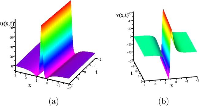
Figure 1. One-soliton solution (u(x, t), v(x, t)) of the SK system (2.13), (2.14) for ${k}_{1}=\tfrac{1}{2}$, σ = − 1, ${\alpha }_{1}=1,{\alpha }_{2}=\mbox{--}1,{\alpha }_{3}=2,{\alpha }_{4}=-\tfrac{3}{2}$, δ1 = δ2 = 0.
(ii) For the KK system (2.24) and (2.25).
Letting $u=\tfrac{3}{2}{\left(\mathrm{ln}(f)\right)}_{{xx}}$ yields the Hirota bilinear form of KK equation as [28, 31, 32]
$\begin{eqnarray}(16{D}_{x}{D}_{t}+{D}_{x}^{6})\{f\cdot f\}+20{D}_{x}^{2}\{f\cdot g\}=0,\end{eqnarray}$
$\begin{eqnarray}{D}_{x}^{4}\{f\cdot f\}-\displaystyle \frac{4}{3}{fg}=0,\end{eqnarray}$
where g is an auxiliary function. Similar to the SK system, we let $U=\tfrac{3}{2}{\left({F}^{-1}\,{F}_{x}\right)}_{x}$ where F = f1I + f2Σ. We determine f1 and f2 by the Hirota method. We get
$\begin{eqnarray}\begin{array}{l}32({{FF}}_{{xt}}-{F}_{x}{F}_{t})+2({{FF}}_{6x}-6{F}_{x}{F}_{5x}+15{F}_{{xx}}{F}_{4x}-10{F}_{{xxx}}^{2})\\ +20({F}_{{xx}}G-2{F}_{x}{G}_{x}+{{FG}}_{{xx}})=0,\end{array}\end{eqnarray}$
$\begin{eqnarray}2({{FF}}_{4x}-4{F}_{x}{F}_{{xxx}}+6{F}_{{xx}}^{2})-\displaystyle \frac{4}{3}{FG}=0,\end{eqnarray}$
which is equivalent to
$\begin{eqnarray}(16{D}_{x}{D}_{t}+{D}_{x}^{6})\{F\cdot F\}+20{D}_{x}^{2}\{F\cdot G\}=0,\end{eqnarray}$
$\begin{eqnarray}{D}_{x}^{4}\{F\cdot F\}-\displaystyle \frac{4}{3}{FG}=0,\end{eqnarray}$
where G = g1I + g2Σ. In componentwise we have
$\begin{eqnarray}\begin{array}{l}(16{D}_{x}{D}_{t}+{D}_{x}^{6})\{{f}_{1}\cdot {f}_{1}+\sigma {f}_{2}\cdot {f}_{2}\}\\ +20{D}_{x}^{2}\{{f}_{1}\cdot {g}_{1}+\sigma {f}_{2}\cdot {g}_{2}\}=0,\end{array}\end{eqnarray}$
$\begin{eqnarray}\begin{array}{l}(16{D}_{x}{D}_{t}+{D}_{x}^{6})\{{f}_{1}\cdot {f}_{2}+{f}_{2}\cdot {f}_{1}\}\\ +20{D}_{x}^{2}\{{f}_{2}\cdot {g}_{1}+{f}_{1}\cdot {g}_{2}\}=0,\end{array}\end{eqnarray}$
$\begin{eqnarray}{D}_{x}^{4}\{{f}_{1}\cdot {f}_{1}+\sigma {f}_{2}\cdot {f}_{2}\}-\displaystyle \frac{4}{3}({f}_{1}{g}_{1}+\sigma {f}_{2}{g}_{2})=0,\end{eqnarray}$
$\begin{eqnarray}{D}_{x}^{4}\{{f}_{2}\cdot {f}_{1}+{f}_{1}\cdot {f}_{2}\}-\displaystyle \frac{4}{3}({f}_{2}{g}_{1}+{f}_{1}{g}_{2})=0.\end{eqnarray}$
To obtain one-soliton solution of the system (2.24), (2.25) we take ${f}_{1}={\alpha }_{0}+{\alpha }_{1}{{\rm{e}}}^{{\theta }_{1}}+{\alpha }_{2}{{\rm{e}}}^{2{\theta }_{1}}$, ${f}_{2}={\alpha }_{3}+{\alpha }_{4}{{\rm{e}}}^{{\theta }_{1}}$, ${g}_{1}={\alpha }_{5}{{\rm{e}}}^{{\theta }_{1}}$, and ${g}_{2}={\alpha }_{6}{{\rm{e}}}^{{\theta }_{1}}$, where θ1 = k1x + ω1t + δ1 for some constants k1, ω1, δ1, and αj, j = 1,…,6. From the above system we get ${\omega }_{1}=-{k}_{1}^{5}$ and the following constraints:
$\begin{eqnarray}\begin{array}{l}{\alpha }_{0}=\displaystyle \frac{{\alpha }_{3}(\sigma {\alpha }_{4}^{2}+{\alpha }_{1}^{2})}{2{\alpha }_{1}{\alpha }_{4}},\,{\alpha }_{2}=\displaystyle \frac{{\alpha }_{1}{\alpha }_{4}}{8{\alpha }_{3}},\\ {\alpha }_{5}=\displaystyle \frac{3}{2}{\alpha }_{1}{k}_{1}^{4},\,{\alpha }_{6}=\displaystyle \frac{3}{2}{\alpha }_{4}{k}_{1}^{4}.\end{array}\end{eqnarray}$
Hence one-soliton solution of the KK system (2.24), (2.25) is given by the pair (u,v)
$\begin{eqnarray}u=\displaystyle \frac{{W}_{1}}{{W}_{2}},\quad v=\displaystyle \frac{{W}_{3}}{{W}_{2}},\end{eqnarray}$
where
$\begin{eqnarray}\begin{array}{rcl}{W}_{1} & = & -12{k}_{1}^{2}{\alpha }_{1}^{2}{\alpha }_{3}{\alpha }_{4}\left[32{\alpha }_{3}^{5}{\alpha }_{4}(7\sigma {\alpha }_{4}^{2}-9{\alpha }_{1}^{2}){\left(\sigma {\alpha }_{4}^{2}-{\alpha }_{1}^{2}\right)}^{2}{{\rm{e}}}^{{\theta }_{1}}\right.\\ & & -16{\alpha }_{1}^{2}{\alpha }_{3}^{4}{\alpha }_{4}^{2}(\sigma {\alpha }_{4}^{2}-{\alpha }_{1}^{2})(23\sigma {\alpha }_{4}^{2}-27{\alpha }_{1}^{2}){{\rm{e}}}^{2{\theta }_{1}}\\ & & -16{\alpha }_{1}^{2}{\alpha }_{3}^{3}{\alpha }_{4}^{3}(\sigma {\alpha }_{4}^{2}-{\alpha }_{1}^{2})(\sigma {\alpha }_{4}^{2}-17{\alpha }_{1}^{2}){{\rm{e}}}^{3{\theta }_{1}}\\ & & +4{\alpha }_{1}^{4}{\alpha }_{3}^{2}{\alpha }_{4}^{4}(23\sigma {\alpha }_{4}^{2}-27{\alpha }_{1}^{2}){{\rm{e}}}^{4{\theta }_{1}}\\ & & +2{\alpha }_{1}^{4}{\alpha }_{3}{\alpha }_{4}^{5}(7\sigma {\alpha }_{4}^{2}-9{\alpha }_{1}^{2}){{\rm{e}}}^{5{\theta }_{1}}-{\alpha }_{4}^{6}{\alpha }_{1}^{6}{{\rm{e}}}^{6{\theta }_{1}}\\ & & \left.+64{\alpha }_{3}^{6}{\left(\sigma {\alpha }_{4}^{2}-{\alpha }_{1}^{2}\right)}^{3}\right],\end{array}\end{eqnarray}$
$\begin{eqnarray}\begin{array}{rcl}{W}_{2} & = & \left[64{\alpha }_{1}^{2}{\alpha }_{3}^{3}{\alpha }_{4}(\sigma {\alpha }_{4}^{2}-{\alpha }_{1}^{2})+8{\alpha }_{1}^{2}{\alpha }_{3}^{2}{\alpha }_{4}^{2}(7\sigma {\alpha }_{4}^{2}-9{\alpha }_{1}^{2}){{\rm{e}}}^{2{\theta }_{1}}\right.\\ & & -16{\alpha }_{1}^{4}{\alpha }_{4}^{3}{\alpha }_{3}{{\rm{e}}}^{3{\theta }_{1}}-{\alpha }_{4}^{4}{\alpha }_{1}^{4}{{\rm{e}}}^{4{\theta }_{1}}\\ & & {\left.-16{\alpha }_{3}^{4}{\left(\sigma {\alpha }_{4}^{2}-{\alpha }_{1}^{2}\right)}^{2}\right]}^{2},\end{array}\end{eqnarray}$
$\begin{eqnarray}\begin{array}{rcl}{W}_{3} & = & -12{k}_{1}^{2}{\alpha }_{4}^{2}{\alpha }_{1}{\alpha }_{3}{{\rm{e}}}^{{\theta }_{1}}\left[64{\alpha }_{1}^{2}{\alpha }_{3}^{2}{\alpha }_{4}{\left(\sigma {\alpha }_{4}^{2}-{\alpha }_{1}^{2}\right)}^{2}{{\rm{e}}}^{{\theta }_{1}}\right.\\ & & -16{\alpha }_{1}^{2}{\alpha }_{3}^{4}{\alpha }_{4}^{2}(11\sigma {\alpha }_{4}^{2}-7{\alpha }_{1}^{2})(\sigma {\alpha }_{4}^{2}-{\alpha }_{1}^{2}){{\rm{e}}}^{2{\theta }_{1}}\\ & & -4{\alpha }_{1}^{4}{\alpha }_{3}^{2}{\alpha }_{4}^{2}(11\sigma {\alpha }_{4}^{2}-7{\alpha }_{1}^{2}){{\rm{e}}}^{4{\theta }_{1}}-4{\alpha }_{1}^{6}{\alpha }_{4}^{5}{\alpha }_{3}{{\rm{e}}}^{5{\theta }_{1}}\\ & & \left.-{\alpha }_{4}^{6}{\alpha }_{1}^{6}{{\rm{e}}}^{6{\theta }_{1}}-64{\alpha }_{3}^{6}{\left(\sigma {\alpha }_{4}^{2}-{\alpha }_{1}^{2}\right)}^{3}\right],\end{array}\end{eqnarray}$
where ${\theta }_{1}={k}_{1}x-{k}_{1}^{5}t+{\delta }_{1}$.

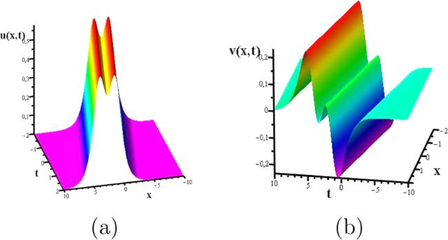
Consider the particular values for the parameters of the solution (5.23) as ${k}_{1}=1,\sigma =-1$, ${\alpha }_{1}={\alpha }_{3}=1,{\alpha }_{4}=2,{\delta }_{1}=0$. We have the solution $(u(x,t),v(x,t))$ where

$\begin{eqnarray}\begin{array}{rcl}u(x,t) & = & 24{{\rm{e}}}^{x-t}\left[59200{{\rm{e}}}^{x-t}+38080{{\rm{e}}}^{2x-2t}\right.\\ & & +\,13440{{\rm{e}}}^{3x-3t}+7616{{\rm{e}}}^{4x-4t}\\ & & \left.+\,2368{{\rm{e}}}^{5x-5t}+64{{\rm{e}}}^{6x-6t}+8000\right]/\left[640{{\rm{e}}}^{x-t}+1184{{\rm{e}}}^{2x-2t}\right.\\ & & {\left.+\,128{{\rm{e}}}^{3x-3t}+16{{\rm{e}}}^{4x-4t}+400\right]}^{2},\end{array}\end{eqnarray}$
$\begin{eqnarray}\begin{array}{rcl}v(x,t) & = & -48{{\rm{e}}}^{x-t}\left[3200{{\rm{e}}}^{x-t}-16320{{\rm{e}}}^{2x-2t}\right.\\ & & \left.+3264{{\rm{e}}}^{4x-4t}-128{{\rm{e}}}^{5x-5t}-64{{\rm{e}}}^{6x-6t}+8000\right]\\ & & /{\left[640{{\rm{e}}}^{x-t}+1184{{\rm{e}}}^{2x-2t}+128{{\rm{e}}}^{3x-3t}+16{{\rm{e}}}^{4x-4t}+400\right]}^{2}.\end{array}\end{eqnarray}$
The graphs of the above solutions are given in figure 2.

Figure 2. One-soliton solution (u(x, t), v(x, t)) of the KK system (2.24), (2.25) for k1 = 1, σ = − 1, α1 = α3 = 1, α4 = 2, δ1 = 0.

We note that taking different expansions for the functions f1 and f2 in (5.4) and (5.5) or ${f}_{1},{f}_{2},{g}_{1},{g}_{2}$ in (5.18)-(5.21) may put strong conditions on the parameters yielding u = 0 or v = 0. For instance, if we use ${f}_{1}={f}_{0}+{{\rm{e}}}^{{k}_{1}x+{\omega }_{1}t+{\delta }_{1}}$, ${f}_{2}={g}_{0}$, where f0, g0 are constants, in the Hirota bilinear form (5.4), (5.5) we get ${\omega }_{1}=-{k}_{1}^{5}$ and also ${g}_{0}=0$ making v = 0. In this case the SK system (2.13), (2.14) for the dynamical variables u and v reduces to the SK equation (2.1) for u.

Since the expressions are quite longer we shall not display two- and three-soliton solutions of the SK and KK systems here. The more interesting case is the soliton solutions of the nonlocal SK and KK equations presented in section 3. They can be easily obtained by using the above soliton solutions of the systems with the reduction formulas (1).a, (1).b, (2).a, and (2).b presented in section 3. These equations will restrict parameters in the soliton solutions (5.7) and (5.23). We shall discuss two- and three-soliton solutions of the SK and KK systems and soliton solutions of the nonlocal SK and KK equations in a forthcoming publication.

6. Concluding remarks

Integrable nonlinear partial differential equations form a special subclass of partial differential equations. They possess Lax pairs which allow the Cauchy problem to be solved by the application of the inverse scattering transform. They possess infinitely many generalized symmetries which imply the existence of a recursion operator. They possess a bi-Hamiltonian structure which indicates the existence of infinitely many conserved quantities. Hence it is an active research area to obtain new integrable equations. There are certain methods for this purpose. For example one of them is the zero curvature formalism and the other one is the prolongation structures. Here in this paper we proposed commuting algebras to produce systems of integrable equations from scalar integrable equations.
We obtained systems of integrable equations with their recursion operators from scalar integrable equations by applying ${{ \mathcal M }}_{2}$-extension. We used this method for SK and KK equations and obtained the SK system and KK system of equations, respectively. Applying the nonlocal reductions to the symmetrical versions of SK and KK systems we obtained eight different new standard nonlocal and eight different new shifted nonlocal integrable differential equations. We also presented one-soliton solutions for the SK and KK systems.

This work is partially supported by the Scientific and Technological Research Council of Turkey (TÜBİTAK).

1
Qi-Liang Z, Man J, Sen-Yue L 2019 Fifth-order Alice-Bob systems and their abundant periodic and solitary wave solutions Commun. Theor. Phys. 71 1149

DOI

2
Qi-Liang Z, Sen-Yue L, Man J 2020 Solitons and soliton molecules in two nonlocal Alice-Bob Sawada-Kotera system Commun. Theor. Phys. 72 060005

DOI

3
Gardner C S, Greene J M, Kruskal M D, Miura R M 1974 Korteweg-de Vries equation and generalizations. VI. Methods for exact solution Commun. Pure Appl. Math. 27 97 133

DOI

4
Ma W X, Fuchssteiner B 1996 Integrable theory of the perturbation equations Chaos Solitons Fractals 7 1227 1250

DOI

5
Ma W X, Zhu Z N 2010 Constructing nonlinear discrete integrable Hamiltonian couplings Comput. Math. Appl. 60 2601 2608

DOI

6
Ma W X 2024 Integrable couplings and two-dimensional unital algebras Axioms 13 481

DOI

7
Gürses M, Pekcan A 2024 How to obtain nonlocal integrable equations in preparation

8
Ablowitz M J, Musslimani Z H 2013 Integrable nonlocal nonlinear Schrödinger equation Phys. Rev. Lett. 110 064105

DOI

9
Ablowitz M J, Musslimani Z H 2016 Inverse scattering transform for the integrable nonlocal nonlinear Schrödinger equation Nonlinearity 29 915 946

DOI

10
Ablowitz M J, Musslimani Z H 2016 Integrable nonlocal nonlinear equations Stud. Appl. Math. 139 7 59

DOI

11
Gürses M, Pekcan A 2018 Nonlocal nonlinear Schrödinger equations and their soliton solutions J. Math. Phys. 59 051501

DOI

12
Gürses M, Pekcan A 2018 Integrable nonlocal reductions Symmetries, Differential Equations and Applications SDEA-III, Istanbul, Turkey, August 2017 266 Kac V G Berlin Springer

13
Gürses M, Pekcan A 2019 Nonlocal nonlinear modified KdV equations and their soliton solutions Commun. Nonlinear Sci. Numer. Simulat. 67 427 448

DOI

14
Ma W X 2023 Integrable nonlocal nonlinear Schrödinger hierarchies of type (−λ*, λ) and soliton solutions Rep. Math. Phys. 92 19 36

DOI

15
Ablowitz M J, Musslimani Z H 2021 Integrable space-time shifted nonlocal nonlinear equations Phys. Lett. A 409 127516

DOI

16
Ablowitz M J, Musslimani Z H, Ossi N J Inverse scattering transform for continuous and discrete space-time shifted integrable equations arXiv:2312.11780v2 [nlin.SI].

17
Gürses M, Pekcan A 2022 Soliton solutions of the shifted nonlocal NLS and MKdV equations Phys. Lett. A 422 127793

DOI

18
Liu S M, Wang J, Zhang D J 2022 Solutions to integrable space-time shifted nonlocal equations Rep. Math. Phys. 89 199 220

DOI

19
Wang X, Wei J 2022 Three types of Darboux transformation and general soliton solutions for the space shifted nonlocal PT symmetric nonlinear Schrödinger equation Appl. Math. Lett. 130 107998

DOI

20
Wang X B, Tian S F 2022 Exotic localized waves in the shifted nonlocal multicomponent nonlinear Schrödinger equation Theor. Math. Phys. 212 1193 1210

DOI

21
Ma W X 2022 N-soliton solutions and the Hirota conditions in (1+1)-dimensions Int. J. Nonlinear Sci. Numer. Simulat. 23 123 133

DOI

22
Gürses M, Karasu A, Sokolov V 1999 On construction of recursion operators from Lax representation J. Math. Phys. 40 6473 6490

DOI

23
Wang J P 2002 A list of 1 + 1 dimensional integrable equations and their properties J. Nonlinear Math. Phys. 9 213 233

DOI

24
Euler M, Euler N 2011 A class of semilinear fifth-order evolution equations: recursion operators and multi potentialisations J. Nonlinear Math. Phys. 18 61 75

DOI

25
Lee C T, Lee C C 2012 Lax pairs and Hamiltonians for the Kaup–Kupershmidt-type equation Phys. Scr. 85 035004

DOI

26
Kaup J D 1980 On the inverse scattering problem for cubic-eigenvalue problems of the class $\Psi$xxx + 6Q$\Psi$x + 6R$\Psi$ = λ$\Psi$ Stud. Appl. Math. 62 189 216

DOI

27
Ma W X 2023 Soliton solutions to constrained nonlocal integrable nonlinear Schrödinger hierarchies of type (−λ, λ) Int. J. Geom. Methods Mod. Phys. 20 2350098

DOI

28
Jimbo M, Miwa T 1983 Solitons and infinite dimensional Lie algebras Publ. Res. Inst. Math. Sci. 19 943

DOI

29
Kazi Sazzad Hossain A K M, Akbar M A 2023 Multi-soliton solutions of the Sawada-Kotera equation using the Hirota direct method: novel insights into nonlinear evolution equations Partial Differ. Equ. Appl. Math. 8 100572

DOI

30
Kumar S, Mohan B 2022 A novel and efficient method for obtaining Hirota's bilinear form for the nonlinear evolution equation in (n+1) dimensions, Partial Differ Equ. Appl. Math. 5 100274

31
Parker A 2000 On soliton solutions of the Kaup–Kupershmidt equation. I. Direct bilinearisation and solitary wave Physica D 137 25 33

DOI

32
Parker A 2000 On soliton solutions of the Kaup–Kupershmidt equation. II. ‘Anomalous' N-soliton solutions Physica D 137 34 48

DOI

Outlines

/