


1. Introduction
2. Preliminaries
3. Monogamy of the unified-(q, s) entanglement
For convenience, we denote ${\rho }_{{A}_{{j}_{1}}| {A}_{{j}_{2}}\cdots {A}_{{j}_{m}}}$ as ${\rho }_{{AB}}$. There exists a pure state decomposition $\{{q}_{i},\left|{\phi }_{i}\right\rangle \}$ such that
Next, we prove that ${g}_{q,s}^{2}({C}^{2}({\rho }_{{AB}}))\leqslant {U}_{q,s}^{2}({\rho }_{{AB}})$. Let $\{{p}_{i},\left|{\omega }_{i}\right\rangle \}$ be the optimal pure state decomposition of ${U}_{q,s}({\rho }_{{AB}})$. Then
For $(q,s)\in { \mathcal R }$, we have
4. Tighter monogamy inequalities in terms of UE
Consider the function $f(x,m)={\left(1+x\right)}^{m}-{p}^{m-1}{x}^{m}$ with $x\geqslant 0$, $1\leqslant p\leqslant 1+\tfrac{1}{x}$ and $m\geqslant 1$. Since $\tfrac{\partial f(x,m)}{\partial x}$ = $m{\left(1+x\right)}^{m-1}-{{mp}}^{m-1}{x}^{m-1}$ = $m[{\left(1+x\right)}^{m-1}-{\left({px}\right)}^{m-1}]\geqslant 0$, the function $f(x,m)$ increases with x. As $x\geqslant h\geqslant 0$, we have $f{(x,m)\geqslant f(h,m)=(1+h)}^{m}-{p}^{m-1}{h}^{m}$. Therefore, we get the inequality (
By straightforward calculation, we have
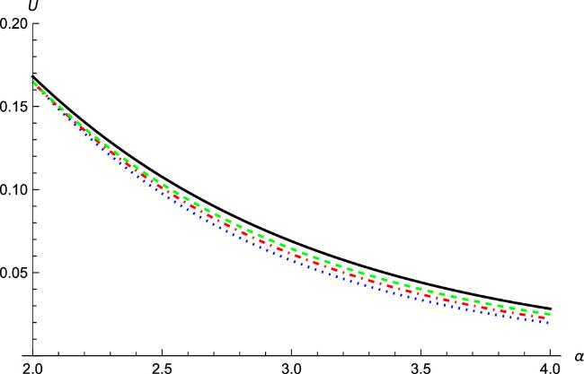
Figure 1. From top to bottom, the black line is the exact values of ${U}_{\mathrm{2,1}}({\rho }_{{P}_{1}| {P}_{2}{P}_{3}})$. The green dashed line (red dot-dashed line) represents the lower bound from our result ( |
From theorem 4, ${U}_{q,s}^{2}({\rho }_{{{AB}}_{i}})\geqslant {h}_{i}{U}_{q,s}^{2}({\rho }_{A| {B}_{i+1}\cdots {B}_{r-1}})$, ${U}_{q,s}^{2}({\rho }_{A| {B}_{i}\cdots {B}_{r-1}})\geqslant {U}_{q,s}^{2}({\rho }_{{{AB}}_{i}})+{\mu }_{i}{U}_{q,s}^{2}({\rho }_{A| {B}_{i+1}\cdots {B}_{r-1}})$, $1\leqslant {p}_{i}\leqslant 1+\tfrac{{\mu }_{i}{U}_{q,s}^{2}({\rho }_{A| {B}_{i+1}\cdots {B}_{r-1}})}{{U}_{q,s}^{2}({\rho }_{{{AB}}_{i}})}$ for $i=1,2,\cdots ,k$. We have
5. Generalized monogamy relation and upper bound for n-qudit systems
For q = 2 and $\tfrac{1}{2}\leqslant s\leqslant 1$ we have
Using the subadditivity of unified-($q,s$) entropy, we have the following inequality,
6. Applications
Table 1. The values of PRE ${{\rm{\Upsilon }}}_{{P}_{11}{P}_{12}| {P}_{21}{P}_{22}}$ for different q and all the possible values of a, denoted by ϒ(q, a, b), when s = 1, m = 4, b = 5, n = 6. |
| q | ϒ(q, 1, 5) | ϒ(q, 2, 5) | ϒ(q, 3, 5) | ϒ(q, 4, 5) |
|---|---|---|---|---|
| 2.0 | 0.191 172 | 0.193 981 | 0.191 172 | 0.183 117 |
| | ||||
| 2.1 | 0.179 591 | 0.182 176 | 0.179 591 | 0.172876 |
| | ||||
| 2.2 | 0.168 899 | 0.171 295 | 0.168 899 | 0.162006 |
| | ||||
| 2.3 | 0.159 022 | 0.161 259 | 0.159 022 | 0.152585 |
| | ||||
| 2.4 | 0.149 893 | 0.151 993 | 0.149 893 | 0.143847 |
Table 2. The values of PRE ${{\rm{\Upsilon }}}_{{P}_{11}{P}_{12}| {P}_{21}{P}_{22}}$ for different q and all the possible values of a, denoted by ϒ(q, a, b), when s = 1, m = 4, b = 6, n = 6. |
| q | ϒ(q, 1, 6) | ϒ(q, 2, 6) | ϒ(q, 3, 6) | ϒ(q, 4, 6) |
|---|---|---|---|---|
| 2.0 | 0.173 999 | 0.183 117 | 0.173 999 | 0.148 145 |
| | ||||
| 2.1 | 0.163 680 | 0.172 876 | 0.163 680 | 0.139568 |
| | ||||
| 2.2 | 0.154 082 | 0.162 006 | 0.154 082 | 0.131526 |
| | ||||
| 2.3 | 0.145 158 | 0.152 585 | 0.145 158 | 0.123996 |
| | ||||
| 2.4 | 0.136 863 | 0.143 847 | 0.136 863 | 0.116952 |
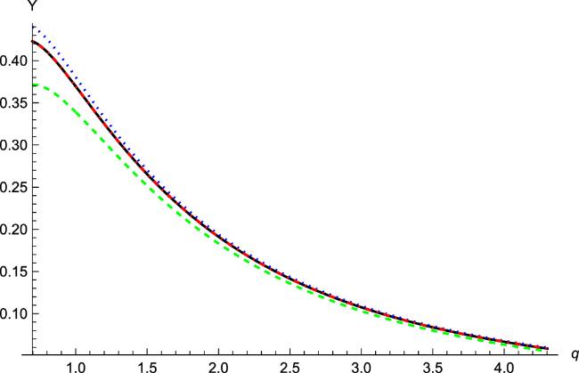
Figure 2. s = 1, m = 4, b = 5, n = 6. From top to bottom, the blue dotted line represents a = 2, the black line represents a = 1, the red dot-dashed line represents a = 3, and the green dashed line represents a = 4. The curves coincide when a = 1 and a = 3. |
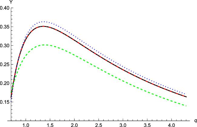
Figure 3. s = 1, m = 4, b = 6, n = 6. From top to bottom, the blue dotted line represents a = 2, the black line represents a = 1, the red dot-dashed line represents a = 3, and the green dashed line represents a = 4. The curves coincide when a = 1 and a = 3. |
Table 3. The values of PRE ${\rm{\Upsilon }}{{\prime} }_{{P}_{11}{P}_{12}| {P}_{21}{P}_{22}}$ for different q and all the possible values of m, denoted by ${\rm{\Upsilon }}^{\prime} (q,m)$, when s = 1 and n = 6. |
| q | ${\rm{\Upsilon }}^{\prime} (q,1)$ | ${\rm{\Upsilon }}^{\prime} (q,2)$ | ${\rm{\Upsilon }}^{\prime} (q,3)$ | ${\rm{\Upsilon }}^{\prime} (q,4)$ | ${\rm{\Upsilon }}^{\prime} (q,5)$ |
|---|---|---|---|---|---|
| 2.0 | 0.077 113 | 0.197 450 | 0.249 914 | 0.197 450 | 0.077113 |
| | |||||
| 2.1 | 0.071 820 | 0.185 350 | 0.235 131 | 0.185350 | 0.071820 |
| | |||||
| 2.2 | 0.067 131 | 0.174 229 | 0.221 395 | 0.174229 | 0.067131 |
| | |||||
| 2.3 | 0.062 961 | 0.163 993 | 0.208 622 | 0.163993 | 0.062961 |
| | |||||
| 2.4 | 0.059 234 | 0.154 560 | 0.196 737 | 0.154560 | 0.059234 |
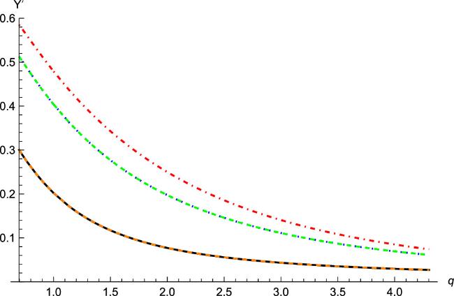
Figure 4. s = 1, n = 6. From top to bottom, the red dot-dashed line represents m = 3, the blue dotted line represents m = 2, the green dashed line represents m = 4, the black line represents m = 1, and the orange dashed line represents m = 5. The curves coincide when m = 1 (m = 2) and m = 5 (m = 4). |