


1. Introduction
As one of the most promising candidates for the realization of quantum information processing and quantum computation, coherent control of quantum superconducting circuits has become a hot topic in the field of quantum optics, which is called circuit quantum electrodynamics (QED) [1–8]. Compared to the traditional cavity QED system, which is realized by coupling the natural atom to the single-mode electromagnetic field in the microcavity, ultrastrong and deep strong coupling between different components of the system can be realized in the circuit QED system. In other words, the coupling strength can be comparable to the frequency of the cavity field or atom (qubit) [9–15]. As a result, the rotating wave approximation can no longer be applied to superconducting circuits.
Photon blockade is an exotic phenomenon in quantum optics. This indicates that the photon exhibits a sub-Poissonian distribution, and the excitation of a single photon prevents simultaneous excitation of the second or subsequent photons. This phenomenon can be predicted by measuring the second-order correlation function g(2)(0), where g(2)(0) ≈ 0 implies a perfect two-photon blockade, and is useful for constructing an ideal single-photon source. A photon blockade was observed in the QED system, which was induced by the strong nonlinearity of the system [16, 17]. An unconventional photon blockade induced by multichannel interference was investigated in detail [18–22]. Moreover, nonreciprocal photon blockade has also been predicted [23, 24]. Considering the microwave regime, it is interesting to investigate photon blockade in superconducting circuits that operate in the ultrastrong coupling regime.
The challenge in the ultrastrong coupling regime is the energy structure modification induced by counter-rotating wave terms. Consequently, the effect of the environment cannot be described by the phenomenal master equation even when we consider the Markovian approximation [25]. In this sense, to deeply understand photon blockade in the ultrastrong coupling regime, we must rederive the master equation in the eigenpresentation of the coupling system.
In this study, we addressed the aforementioned issue by considering a transmon–transmon coupling system. Beginning with the Lagrangian of the system, we obtained the Hamiltonian using the Legendre transformation and predicted the ultrastrong coupling with the available experimental parameters. Then, the exact diagonalization of the full Hamiltonian [26, 27] allowed us to obtain the master equation and discuss the photon blockade. In addition, we illustrate the optimal parameter for the realization of photon blockade and compare the results with those of the rotating wave approximation.
2. Model and Hamiltonian
The system under consideration is composed of a pair of transmons, as illustrated in figure 1. The Lagrangian of the coupled system is given by [28]
$\begin{eqnarray}\begin{array}{rcl}{ \mathcal L } & = & \displaystyle \frac{{C}_{1}}{2}{\dot{\psi }}_{1}^{2}+\displaystyle \frac{{C}_{2}}{2}{\dot{\psi }}_{2}^{2}-\displaystyle \frac{{\psi }_{1}^{2}}{2{L}_{1}}-\displaystyle \frac{{\psi }_{2}^{2}}{2{L}_{2}}\\ & & +{E}_{{\rm{J}}1}\cos \left(\displaystyle \frac{{\psi }_{1}}{{\phi }_{0}}\right)+{E}_{{\rm{J}}2}\cos \left(\displaystyle \frac{{\psi }_{2}}{{\phi }_{0}}\right)+\displaystyle \frac{{C}_{{\rm{J}}}}{2}{\left(\dot{{\psi }_{1}}-{\dot{\psi }}_{2}\right)}^{2},\end{array}\end{eqnarray}$
where Ci, Li, EJi, and ψi (i = 1, 2) are the capacitance, inductance, Josephson energy, and phase of the ith transmon, respectively. CJ is the capacitance that couples the two transmons, and φ0 is the reduced flux quantum. We introduce the conjugate node charge ${Q}_{i}=\partial { \mathcal L }/\partial {\dot{\psi }}_{i}$ and follow the standard quantization procedure. The Hamiltonian can be obtained as $\begin{eqnarray}\begin{array}{rcl}H & = & {Q}_{1}{\dot{\psi }}_{1}+{Q}_{2}{\dot{\psi }}_{2}-{ \mathcal L }\\ & = & \displaystyle \sum _{i=1}^{2}\left[\displaystyle \frac{{Q}_{1}^{2}}{2{C}_{{\rm{T}}i}}+\displaystyle \frac{{\psi }_{1}^{2}}{2{L}_{i}}-{E}_{{\rm{J}}i}\cos (\displaystyle \frac{{\psi }_{i}}{{\phi }_{0}})\right]+\displaystyle \frac{{Q}_{1}{Q}_{2}}{{C}_{\mathrm{int}}},\end{array}\end{eqnarray}$
where $\begin{eqnarray}{C}_{{\rm{T}}i}=\displaystyle \frac{({C}_{1}+{C}_{{\rm{J}}})({C}_{2}+{C}_{{\rm{J}}})-{C}_{{\rm{J}}}^{2}}{{C}_{3-i}+{C}_{{\rm{J}}}},\end{eqnarray}$
$\begin{eqnarray}{C}_{\mathrm{int}}=\displaystyle \frac{({C}_{1}+{C}_{{\rm{J}}})({C}_{2}+{C}_{{\rm{J}}})-{C}_{{\rm{J}}}^{2}}{{C}_{{\rm{J}}}}.\end{eqnarray}$
The Hamiltonian can be further divided into three terms as H = H0 + HU + HI, where $\begin{eqnarray}{H}_{0}=\displaystyle \sum _{i=1,2}\left(\displaystyle \frac{{Q}_{i}^{2}}{2{C}_{{\rm{T}}i}}+\displaystyle \frac{{\psi }_{i}^{2}}{2{L}_{{\rm{T}}i}}\right),\end{eqnarray}$
$\begin{eqnarray}{H}_{{\rm{U}}}=-\displaystyle \sum _{i=1,2}{E}_{{\rm{J}}i}\left[\cos (\displaystyle \frac{{\psi }_{i}}{{\phi }_{0}})-1+\displaystyle \frac{{\psi }_{i}^{2}}{2{\phi }_{0}^{2}}\right],\end{eqnarray}$
$\begin{eqnarray}{H}_{{\rm{I}}}=\displaystyle \frac{{Q}_{1}{Q}_{2}}{{C}_{\mathrm{int}}}.\end{eqnarray}$
H0 is the linear part of the two transmons with $\begin{eqnarray}\displaystyle \frac{1}{{L}_{{\rm{T}}i}}=\displaystyle \frac{1}{{L}_{i}}+\displaystyle \frac{{E}_{{\rm{J}}i}}{{\phi }_{0}^{2}}.\end{eqnarray}$
HU represents the nonlinear parts of the transmons, and HI is their interaction.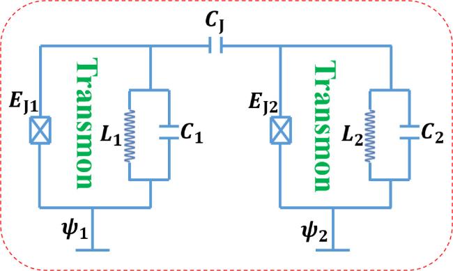
Figure 1. Schematic of a pair of transmons that couple to each via capacity CJ. Ci, Li, EJi, and ψi (where i = 1, 2) are the capacitance, inductance, Josephson energy, and the phase of the ith transmon, respectively. |
Defining the dimensionless charge and phase variables by $({E}_{{\rm{L}}i}={\phi }_{0}^{2}/{L}_{{\rm{T}}i},\,{E}_{{\rm{C}}i}={e}^{2}/2{C}_{{\rm{T}}i})$ 11 ) represents the free term of the two transmons. Equation (13 ) represents their interaction, where we consider both the rotating wave terms ${a}_{1}^{\dagger }{a}_{2}+{a}_{2}^{\dagger }{a}_{1}$ and counter-rotating wave terms ${a}_{1}^{\dagger }{a}_{2}^{\dagger }+{a}_{1}{a}_{2}$. It is interesting to note that the small quantity εi (where i = 1, 2) comes from the commute relation of $[{a}_{i},{a}_{j}^{\dagger }]={\delta }_{i,j}$. This term reflects the effect of the quantum fluctuation.
$\begin{eqnarray}\displaystyle \frac{{Q}_{i}}{2e}={\left(\tfrac{{E}_{{\rm{L}}i}}{8{E}_{{\rm{C}}i}}\right)}^{\tfrac{1}{4}}{q}_{i},\displaystyle \frac{{\psi }_{i}}{{\phi }_{0}}={\left(\tfrac{8{E}_{{\rm{C}}i}}{{E}_{{\rm{L}}i}}\right)}^{\tfrac{1}{4}}{\varphi }_{i},\end{eqnarray}$
and introducing the bosonic annihilation and creation operators $\begin{eqnarray}{a}_{i}=\displaystyle \frac{{\varphi }_{i}+{\rm{i}}{q}_{i}}{\sqrt{2}},{a}_{i}^{\dagger }=\displaystyle \frac{{\varphi }_{i}-{\rm{i}}{q}_{i}}{\sqrt{2}},\end{eqnarray}$
we can achieve the second quantization Hamiltonian $\begin{eqnarray}{H}_{0}=\displaystyle \sum _{i=1,2}{\hslash }{\delta }_{i}{a}_{i}^{\dagger }{a}_{i},\end{eqnarray}$
$\begin{eqnarray}{H}_{{\rm{U}}}=-\displaystyle \sum _{i=1,2}{U}_{i}{a}_{i}^{\dagger }{a}_{i}^{\dagger }{a}_{i}{a}_{i},\end{eqnarray}$
$\begin{eqnarray}{H}_{{\rm{I}}}=J({a}_{1}^{\dagger }{a}_{2}+{a}_{2}^{\dagger }{a}_{1}-{a}_{1}^{\dagger }{a}_{2}^{\dagger }-{a}_{2}^{\dagger }{a}_{1}^{\dagger }),\end{eqnarray}$
where $\begin{eqnarray}\hslash {\delta }_{i}=\sqrt{8{E}_{{\rm{C}}i}{E}_{{\rm{L}}i}}-\sqrt{\displaystyle \frac{2{E}_{{\rm{J}}i}^{2}{E}_{{\rm{C}}i}}{{E}_{{\rm{L}}i}}}(1-{{\rm{e}}}^{-\tfrac{{\epsilon }_{i}}{4}}),\end{eqnarray}$
$\begin{eqnarray}{\epsilon }_{i}=\sqrt{\displaystyle \frac{8{E}_{{\rm{C}}i}}{{E}_{{\rm{L}}i}}},\end{eqnarray}$
$\begin{eqnarray}{U}_{i}=\displaystyle \frac{{E}_{{\rm{J}}i}{E}_{{\rm{C}}i}}{{E}_{{\rm{L}}i}}{{\rm{e}}}^{-\tfrac{{\epsilon }_{i}}{4}},\end{eqnarray}$
$\begin{eqnarray}J=\displaystyle \frac{2{e}^{2}}{{C}_{\mathrm{int}}}{\left(\tfrac{{E}_{{\rm{L}}1}{E}_{{\rm{L}}2}}{64{E}_{{\rm{C}}1}{E}_{{\rm{C}}2}}\right)}^{\tfrac{1}{4}}.\end{eqnarray}$
Equation (In what follows, we set the inductances L1 = L2 = ∞ , capacitances C1 = C2 = C, and Josephson energies EJ1 = EJ2 = EJ. As a result, we can achieve the symmetry condition δ1 = δ2 = δ, U1 = U2 = U, and ε1 = ε2 = ε.
In figure 2(a), we plot the curve of J/δ as a function of the capacity CJ, which couples the two transmons. As shown in the figure, the ratio J/δ increases monotonously with an increase in CJ and achieves an ultrastrong coupling regime J/δ > 0.1 when CJ/C > 0.5. This is why we must consider the counter-rotating wave coupling terms in equation (13 ). Meanwhile, as shown in figure 2(b), we investigated the nonlinear interaction strength U as a function of CJ. This shows that U is much smaller than J, implying that we are working in a weak nonlinear interaction regime. As a result, in the Hamiltonian HU, it is safe to neglect the counter-rotating wave terms, such as ${a}_{i}^{4},{a}_{i}^{\dagger }{a}_{i}^{3}$, and so on.
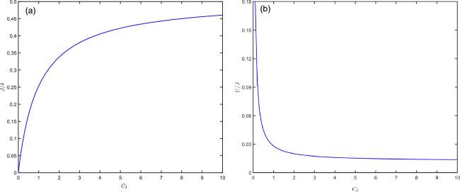
Figure 2. Parameters of (a) J/δ and (b) U/J as functions of coupling capacity CJ. The other parameters were set as C = 1 μF and EJ/(ℏ) = 200 MHz. |
Now, we perform the diagonalization of the Hamiltonian HL = H0 + HI, which yields [26, 27]
$\begin{eqnarray}{H}_{{\rm{L}}}={E}_{+}{c}_{+}^{\dagger }{c}_{+}+{E}_{-}{c}_{-}^{\dagger }{c}_{-},\end{eqnarray}$
where ${E}_{\pm }=\sqrt{{\delta }^{2}\pm 2J\delta }$ and $\begin{eqnarray}{c}_{\pm }=\displaystyle \frac{1}{\sqrt{8\delta {E}_{\pm }}}[({E}_{\pm }+\delta )({a}_{1}\pm {a}_{2})-({E}_{\pm }-\delta )({a}_{1}^{\dagger }\pm {a}_{2}^{\dagger })].\end{eqnarray}$
Then, the inverse transformation is given by $\begin{eqnarray}{a}_{1}=\displaystyle \frac{1}{\sqrt{8\delta }}\left({{ \mathcal K }}_{+}{c}_{+}+{{ \mathcal K }}_{-}{c}_{-}+{{ \mathcal T }}_{+}{c}_{+}^{\dagger }+{{ \mathcal T }}_{-}{c}_{-}^{\dagger }\right),\end{eqnarray}$
$\begin{eqnarray}{a}_{2}=\displaystyle \frac{1}{\sqrt{8\delta }}\left({{ \mathcal K }}_{+}{c}_{+}-{{ \mathcal K }}_{-}{c}_{-}+{{ \mathcal T }}_{+}{c}_{+}^{\dagger }-{{ \mathcal T }}_{-}{c}_{-}^{\dagger }\right),\end{eqnarray}$
where ${{ \mathcal K }}_{\pm }=({E}_{\pm }+\delta )/\sqrt{{E}_{\pm }},{{ \mathcal T }}_{\pm }=({E}_{\pm }-\delta )/\sqrt{{E}_{\pm }}$.In terms of c+, c−, and their Hermitian, the nonlinear term HU can be expressed as
$\begin{eqnarray}\begin{array}{rcl}{H}_{{\rm{U}}} & = & \displaystyle \sum _{i=\pm }\left({\delta }_{i}{c}_{i}^{\dagger }{c}_{i}-{U}_{i}{c}_{i}^{\dagger }{c}_{i}^{\dagger }{c}_{i}{c}_{i}\right)\\ & & -{U}_{{\rm{I}}}\left(4{c}_{+}^{\dagger }{c}_{+}{c}_{-}^{\dagger }{c}_{-}+{c}_{+}^{\dagger }{c}_{+}^{\dagger }{c}_{-}{c}_{-}+{c}_{-}^{\dagger }{c}_{-}^{\dagger }{c}_{+}{c}_{+}\right),\end{array}\end{eqnarray}$
where $\begin{eqnarray}{\delta }_{\pm }=-\displaystyle \frac{{E}_{{\rm{J}}}{E}_{\pm }\epsilon }{2\omega }[1-{{\rm{e}}}^{-\tfrac{\epsilon }{8\omega }({E}_{+}+{E}_{-})}],\end{eqnarray}$
$\begin{eqnarray}{U}_{\pm }={E}_{{\rm{J}}}\displaystyle \frac{{E}_{\pm }^{2}{\epsilon }^{2}}{32{\omega }^{2}}{{\rm{e}}}^{-\tfrac{\epsilon }{8\omega }({E}_{+}+{E}_{-})},\end{eqnarray}$
$\begin{eqnarray}{U}_{{\rm{I}}}={E}_{{\rm{J}}}\displaystyle \frac{{E}_{+}{E}_{-}{\epsilon }^{2}}{32{\omega }^{2}}{{\rm{e}}}^{-\tfrac{\epsilon }{8\omega }({E}_{+}+{E}_{-})}.\end{eqnarray}$
Therefore, the nonlinear interaction strengths satisfy ${U}_{+}={\left({E}_{+}/{E}_{-}\right)}^{2}{U}_{-}$ and UI = (E+/E−)U−.3. Master equation
Now, we discuss the effect of the external environment on the coupled transmon system via the master equation approach. As shown in figure 2(b), the nonlinear coupling strength U is much weaker than the linear coupling J; therefore, we will not consider the nonlinear terms in the derivation of the master equation under the Markovian approximation but only treat them in a phenomenological manner. To this end, we write the transmon–environment interaction Hamiltonian as H = Hs + HB + V, where
$\begin{eqnarray}\begin{array}{rcl}{H}_{{\rm{s}}} & = & \omega ({a}_{1}^{\dagger }{a}_{1}+{a}_{2}^{\dagger }{a}_{2})+J({a}_{1}^{\dagger }{a}_{2}+{a}_{2}^{\dagger }{a}_{1}-{a}_{1}^{\dagger }{a}_{2}^{\dagger }-{a}_{2}^{\dagger }{a}_{1}^{\dagger })\\ & = & {E}_{+}{c}_{+}^{\dagger }{c}_{+}+{E}_{-}{c}_{-}^{\dagger }{c}_{-},\end{array}\end{eqnarray}$
$\begin{eqnarray}{H}_{{\rm{B}}}=\displaystyle \sum _{i}{\omega }_{{\rm{b}}i}{b}_{i}^{\dagger }{b}_{i}+\displaystyle \sum _{i}{\omega }_{{\rm{d}}i}{d}_{i}^{\dagger }{d}_{i},\end{eqnarray}$
$\begin{eqnarray}V=\displaystyle \sum _{i}{f}_{i}({b}_{i}^{\dagger }{a}_{1}+{b}_{i}{a}_{1}^{\dagger })+\displaystyle \sum _{i}{g}_{i}({d}_{i}^{\dagger }{a}_{2}+{d}_{i}{a}_{2}^{\dagger }).\end{eqnarray}$
Here, bi (di) is the ith mode in the reservoir, which interacts with transmon a1 (a2) with a frequency ωbi (ωdi) and coupling strength fi (gi).In terms of c+ and c−, the interaction Hamiltonian V becomes time dependent as (in the interaction representation)
$\begin{eqnarray}\begin{array}{rcl}V(t) & = & \displaystyle \sum _{i}\displaystyle \frac{{f}_{i}}{\sqrt{8\omega }}[{{ \mathcal K }}_{+}{b}_{i}^{\dagger }{c}_{+}{{\rm{e}}}^{{\rm{i}}({\omega }_{{\rm{b}}i}-{E}_{+})t}\\ & & +{{ \mathcal K }}_{-}{b}_{i}{c}_{-}{{\rm{e}}}^{{\rm{i}}({\omega }_{{\rm{b}}i}-{E}_{-})t}]+{\rm{H}}.{\rm{c}}.\\ & & +\displaystyle \sum _{i}\displaystyle \frac{{g}_{i}}{\sqrt{8\omega }}[{{ \mathcal K }}_{+}{d}_{i}^{\dagger }{c}_{+}{{\rm{e}}}^{{\rm{i}}({\omega }_{{\rm{d}}i}-{E}_{+})t}\\ & & +{{ \mathcal K }}_{-}{d}_{i}^{\dagger }{c}_{-}{{\rm{e}}}^{{\rm{i}}({\omega }_{{\rm{d}}i}-{E}_{-})t}]+{\rm{H}}.{\rm{c}}.,\end{array}\end{eqnarray}$
where ${{ \mathcal K }}_{\pm }=({E}_{\pm }+\omega )/\sqrt{{E}_{\pm }}$.Under the Markov approximation, the master equation in the interaction representation (defined by H0 = Hs + HB) is written as [25]
$\begin{eqnarray}\displaystyle \frac{{\rm{d}}{\rho }_{{\rm{I}}}}{{\rm{d}}t}=-{\int }_{0}^{\infty }{\rm{d}}s{\mathrm{Tr}}_{{\rm{B}}}[V(t),[V(t-s),{\rho }_{{\rm{I}}}(t)\otimes {\rho }_{{\rm{B}}}]],\end{eqnarray}$
where ρB is the density matrix of the reservoirs.At zero temperature, the master equation for our system (in the Schödinger representation) is obtained as
$\begin{eqnarray}\begin{array}{rcl}\displaystyle \frac{{\rm{d}}}{{\rm{d}}t}\rho & = & -{\rm{i}}[\displaystyle \sum _{i=\pm }{E}_{i}{c}_{i}^{\dagger }{c}_{i},\rho ]\\ & & +\displaystyle \sum _{i=\pm }\displaystyle \frac{\kappa {{ \mathcal K }}_{i}^{2}}{4\omega }(2{c}_{i}\rho {c}_{i}^{\dagger }-{c}_{i}^{\dagger }{c}_{i}\rho -\rho {c}_{i}^{\dagger }{c}_{i}),\end{array}\end{eqnarray}$
where κ is the decay rate defined by the spectrum of the reservoirs ${\kappa }_{1}(\omega )={\sum }_{i}{f}_{i}^{2}\delta ({\omega }_{{\rm{b}}i}-\omega ),{\kappa }_{2}(\omega )={\sum }_{i}{g}_{i}^{2}\delta ({\omega }_{{\rm{d}}i}-\omega )$, and we considered the case of κ1(ω) = κ2(ω) = κ.Finally, we compare the master equation with the case in which the rotating wave approximation is applied in the transmon–transmon coupling Hamiltonian. That is,
$\begin{eqnarray}{H}_{{\rm{s}}}=\omega ({a}_{1}^{\dagger }{a}_{1}+{a}_{2}^{\dagger }{a}_{2})+J({a}_{1}^{\dagger }{a}_{2}+{a}_{2}^{\dagger }{a}_{1}).\end{eqnarray}$
An immediate result yields E± = ω ± J and ${c}_{\pm }=({a}_{1}\pm {a}_{2})/\sqrt{2}$, and the master equation becomes $\begin{eqnarray}\displaystyle \frac{{\rm{d}}}{{\rm{d}}t}\rho =-{\rm{i}}[{H}_{{\rm{s}}},\rho ]+\displaystyle \sum _{i=\pm }\kappa (2{c}_{i}\rho {c}_{i}^{\dagger }-{c}_{i}^{\dagger }{c}_{i}\rho -\rho {c}_{i}^{\dagger }{c}_{i}).\end{eqnarray}$
Furthermore, we introduce coherent driving to the first transmon a1 with frequency ωd, and the driving Hamiltonian is given by $\begin{eqnarray}{H}_{{\rm{d}}}=\eta \cos ({\omega }_{{\rm{d}}}t)({a}_{1}^{\dagger }+{a}_{1}).\end{eqnarray}$
Moving to the eigenstate representation and performing the rotating wave approximation, the driving Hamiltonian becomes $\begin{eqnarray}{H}_{{\rm{d}}}={\eta }_{0}[({c}_{+}^{\dagger }+{c}_{-}^{\dagger }){{\rm{e}}}^{-{\rm{i}}{\omega }_{{\rm{d}}}t}+({c}_{+}+{c}_{-}){{\rm{e}}}^{{\rm{i}}{\omega }_{{\rm{d}}}t}],\end{eqnarray}$
where $\begin{eqnarray}{\eta }_{0}=\displaystyle \frac{\eta (\sqrt{{E}_{+}}+\sqrt{{E}_{-}})}{\sqrt{8\omega }}.\end{eqnarray}$
Now, we consider the nonlinear terms in a phenomenological manner and work in the rotating frame with driving frequency ωd. The master equation becomes $\begin{eqnarray}\displaystyle \frac{{\rm{d}}}{{\rm{d}}t}\rho =-{\rm{i}}[{{ \mathcal H }}_{{\rm{T}}},\rho ]+\displaystyle \sum _{i=\pm }\displaystyle \frac{\kappa {{ \mathcal K }}_{i}^{2}}{4\omega }(2{c}_{i}\rho {c}_{i}^{\dagger }-{c}_{i}^{\dagger }{c}_{i}\rho -\rho {c}_{i}^{\dagger }{c}_{i}),\end{eqnarray}$
where $\begin{eqnarray}\begin{array}{rcl}{{ \mathcal H }}_{{\rm{T}}} & = & \displaystyle \sum _{i=\pm }\left({{\rm{\Delta }}}_{i}{c}_{i}^{\dagger }{c}_{i}-{U}_{i}{c}_{i}^{\dagger }{c}_{i}^{\dagger }{c}_{i}{c}_{i}\right)\\ & & -{U}_{{\rm{I}}}\left(4{c}_{+}^{\dagger }{c}_{+}{c}_{-}^{\dagger }{c}_{-}+{c}_{+}^{\dagger }{c}_{+}^{\dagger }{c}_{-}{c}_{-}+{c}_{-}^{\dagger }{c}_{-}^{\dagger }{c}_{+}{c}_{+}\right)\\ & & +{\eta }_{0}\left({c}_{+}^{\dagger }+{c}_{-}^{\dagger }+{c}_{+}+{c}_{-}\right),\end{array}\end{eqnarray}$
and Δ± = δ± − ωd.4. Photon blockade
In the preceding sections, we obtained the master equation for the coupled transmon system. Under external driving and intrinsic dissipation, the system finally evolved into a steady state. To investigate the application of our system in a single-photon source, we continue to study photon blockade, which is quantified by the equal-time second-order correlation function42 , 43 ) can be approximated by44 ) becomes
$\begin{eqnarray}{g}_{\pm }^{(2)}(0)=\displaystyle \frac{\left\langle {c}_{\pm }^{\dagger }{c}_{\pm }^{\dagger }{c}_{\pm }{c}_{\pm }\right\rangle }{{\left\langle {c}_{\pm }^{\dagger }{c}_{\pm }\right\rangle }^{2}}.\end{eqnarray}$
As the first step, we try to find the optimal condition to realize the photon blockade for the ith eigenmode, i.e. ${g}_{i}^{(2)}\approx 0$. Because we consider a weak driving situation with η ≪ κ, it is reasonable to truncate the Hilbert space up to two excitation subspaces. Therefore, we approximated the wave function of the system as [29–31] $\begin{eqnarray}\begin{array}{rcl}| \psi \rangle & = & {D}_{00}| 0;0\rangle +{D}_{01}| 0;1\rangle +{D}_{10}| 1;0\rangle \\ & & +{D}_{20}| 2;0\rangle +{D}_{11}| 1;1\rangle +{D}_{02}| 0;2\rangle ,\end{array}\end{eqnarray}$
where ∣n+; n−⟩ represents the Fock state with n+ photons in c+ mode and n− photons in c− mode. Then, the Schrödinger equation gives $\begin{eqnarray}{\rm{i}}\displaystyle \frac{{\rm{d}}}{{\rm{d}}t}{D}_{00}={\eta }_{0}({D}_{01}+{D}_{10}),\end{eqnarray}$
$\begin{eqnarray}{\rm{i}}\displaystyle \frac{{\rm{d}}}{{\rm{d}}t}{D}_{10}=({{\rm{\Delta }}}_{+}-{\rm{i}}{{ \mathcal K }}_{+}){D}_{10}+{\eta }_{0}({D}_{00}+{D}_{11})+\sqrt{2}{\eta }_{0}{D}_{20}\end{eqnarray}$
$\begin{eqnarray}{\rm{i}}\displaystyle \frac{{\rm{d}}}{{\rm{d}}t}{D}_{01}=({{\rm{\Delta }}}_{-}-{\rm{i}}{{ \mathcal K }}_{-}){D}_{01}+{\eta }_{0}({D}_{00}+{D}_{11})+\sqrt{2}{\eta }_{0}{D}_{02},\end{eqnarray}$
$\begin{eqnarray}{\rm{i}}\displaystyle \frac{{\rm{d}}}{{\rm{d}}t}{D}_{20}=2({{\rm{\Delta }}}_{+}-{U}_{+}-{\rm{i}}{{ \mathcal K }}_{+}){D}_{20}+\sqrt{2}{\eta }_{0}{D}_{10}-2{U}_{I}{D}_{02},\end{eqnarray}$
$\begin{eqnarray}{\rm{i}}\displaystyle \frac{{\rm{d}}}{{\rm{d}}t}{D}_{02}=2({{\rm{\Delta }}}_{-}-{U}_{-}-{\rm{i}}{{ \mathcal K }}_{-}){D}_{02}+\sqrt{2}{\eta }_{0}{D}_{01}-2{U}_{I}{D}_{20},\end{eqnarray}$
$\begin{eqnarray}\begin{array}{rcl}{\rm{i}}\displaystyle \frac{{\rm{d}}}{{\rm{d}}t}{D}_{11} & = & [{{\rm{\Delta }}}_{+}+{{\rm{\Delta }}}_{-}-{U}_{I}-{\rm{i}}({{ \mathcal K }}_{+}+{{ \mathcal K }}_{-})]{D}_{11}\\ & & +{\eta }_{0}({D}_{01}+{D}_{10}).\end{array}\end{eqnarray}$
In the condition of weak driving η ≪ κ, we have [32] $\begin{eqnarray}| {D}_{00}| \gg \{| {D}_{01}| ,| {D}_{10}| \}\gg \{| {D}_{20}| ,| {D}_{11}| ,| {D}_{02}| \}.\end{eqnarray}$
Therefore, the single-photon equation in equations ( $\begin{eqnarray}({{\rm{\Delta }}}_{+}-{\rm{i}}{{ \mathcal K }}_{+}){D}_{10}=-{\eta }_{0}{D}_{00},\end{eqnarray}$
$\begin{eqnarray}({{\rm{\Delta }}}_{-}-{\rm{i}}{{ \mathcal K }}_{-}){D}_{01}=-{\eta }_{0}{D}_{00},\end{eqnarray}$
which yields $\begin{eqnarray}\displaystyle \frac{{D}_{01}}{{D}_{10}}=\displaystyle \frac{{{\rm{\Delta }}}_{+}-{\rm{i}}{{ \mathcal K }}_{+}}{{{\rm{\Delta }}}_{-}-{\rm{i}}{{ \mathcal K }}_{-}}=\displaystyle \frac{1}{\chi }.\end{eqnarray}$
As a result, the two-photon equation ( $\begin{eqnarray}2({{\rm{\Delta }}}_{+}-{U}_{+}-{\rm{i}}{{ \mathcal K }}_{+}){D}_{20}+\sqrt{2}{\eta }_{0}\chi {D}_{01}-2{U}_{I}{D}_{02}=0.\end{eqnarray}$
We now consider the case in which the photon blockade occurs in the c+ mode by setting ${g}_{+}^{(2)}(0)\ll 1$ with D20 = 0. It then yields $\begin{eqnarray}2({{\rm{\Delta }}}_{-}-{U}_{-}-{\rm{i}}{{ \mathcal K }}_{-}){D}_{02}+\sqrt{2}{\eta }_{0}{D}_{01}=0,\end{eqnarray}$
$\begin{eqnarray}\sqrt{2}{\eta }_{0}\chi {D}_{01}-2{U}_{{\rm{I}}}{D}_{02}=0{\rm{.}}\end{eqnarray}$
The optimal parameter condition for the realization of photon blockade can be determined using the presented equations, in which the determinate of the coefficient matrix for D01 and D02 is zero. Then, we obtain $\begin{eqnarray}{{\rm{\Delta }}}_{-}^{2}-{{ \mathcal K }}_{-}^{2}+{U}_{{\rm{I}}}{{\rm{\Delta }}}_{+}-{U}_{-}{{\rm{\Delta }}}_{-}=0,\end{eqnarray}$
$\begin{eqnarray}{U}_{-}{{ \mathcal K }}_{-}-2{{\rm{\Delta }}}_{-}{{ \mathcal K }}_{-}-{U}_{{\rm{I}}}{{ \mathcal K }}_{+}=0{\rm{.}}\end{eqnarray}$
Following the same procedure, we can obtain the optimal condition for the blockade of the c− mode, but this cannot be satisfied. Therefore, we discuss only the photon blockade of the c+ mode.In figure 3, we plot the optimal driving frequency ωopt and optical decay rate κopt as a function of the coupling strength J based on equations (54 ) and (55 ). We found that the optimal frequency of the driving field decreased with coupling strength. Moreover, under the ultrastrong coupling condition, for example, J/ω = 0.35, we observed that κopt/ω ≈ 0.5 within the parameter U−/ω = 0.2. Therefore, the optimal decay rate can be larger than the strength of the nonlinear interaction, i.e. κopt/U > 1. In other words, the system works in an unconventional photon-blockade regime.
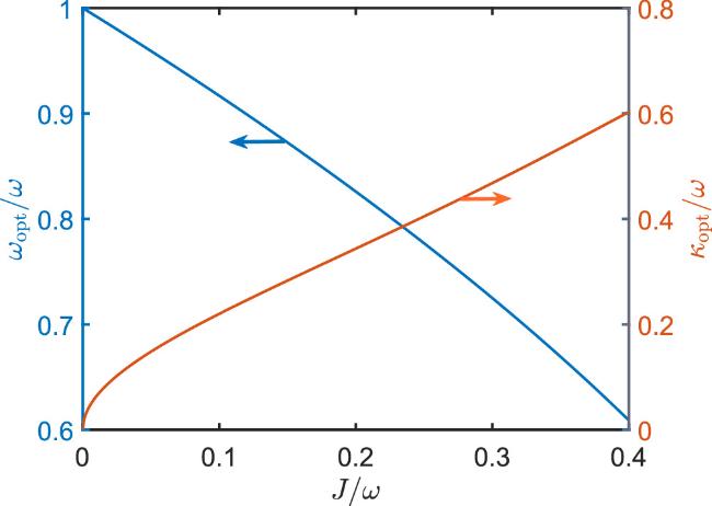
Figure 3. Optimal parameter regime for the photon blockade in c+ beyond the rotating wave approximation. The parameter was set as U−/ω = 0.2. |
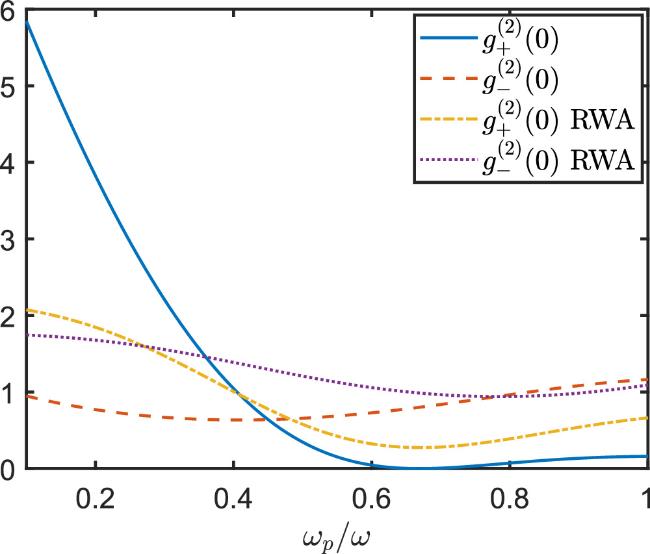
Furthermore, based on the master equation, we numerically plotted the photonic second-order correlation for both the c+ and c− modes within and beyond the rotating wave approximation in figure 4. This demonstrates that a perfect photon blockade of the c− mode cannot be realized in the considered parameter regime. Furthermore, the counter-rotating wave terms not only displaced the optimal driving frequency, but also qualitatively enhanced the blockade behavior. This can be verified by observing that the value of ${g}_{+}^{(2)}(0)$ is much smaller for the case beyond the rotating wave approximation (solid blue line) than that within it (dotted–dashed yellow line).
Figure 4. Second-order correlation function for the c+ and c− modes within and beyond the rotating wave approximation based on the master equations. The parameters were set as J/ω = 0.35 and U−/ω = 0.2. |
5. Conclusions
We studied ultrastrong coupling in a double-transmon system. In the realistic experimental setup, the Josephson energy of the transmon qubit can be achieved by EJ/(2πℏ) ≈ 6 ∼ 10 GHz. The resonant frequencies of the transmons are on the order of gigahertz [33–36], and their coupling strength can be tuned from tens to hundreds of megahertz.
In summary, we diagonalized the Hamiltonian and obtained the Markovian master equation beyond the phenomenological treatment. To discuss the quantum nature of the system, we investigated the photon blockade by predicting the optimal parameter and showed the numerical results based on the global master equation. A comparison with the results of the rotating wave approximation highlights the effect of ultrastrong transmon–transmon coupling.