Welcome to visit Communications in Theoretical Physics,
Quantum Physics and Quantum Information

Masking quantum information in multipartite systems via Fourier and Hadamard matrices*

  • Chen-Ming Bai , ** ,
  • Meng-Ya Wang ,
  • Su-Juan Zhang ,
  • Lu Liu
Expand
  • Department of Mathematics and Physics, Shijiazhuang Tiedao University, Shijiazhuang 050043, China

**Author to whom any correspondence should be addressed.

Received date: 2024-07-02

  Revised date: 2024-09-27

  Accepted date: 2024-09-29

  Online published: 2024-11-27

Supported by

National Natural Science Foundation of China(No.12301590)

Natural Science Foundation of Hebei Province(No.A2022210002)

Copyright

© 2024 Institute of Theoretical Physics CAS, Chinese Physical Society and IOP Publishing. All rights, including for text and data mining, AI training, and similar technologies, are reserved.

Abstract

Quantum information masking (QIM) is a crucial technique for protecting quantum data from being accessed by local subsystems. In this paper, we introduce a novel method for achieving 1-uniform QIM in multipartite systems utilizing a Fourier matrix. We further extend this approach to construct an orthogonal array with the aid of a Hadamard matrix, which is a specific type of Fourier matrix. This allows us to explore the relationship between 2-uniform QIM and orthogonal arrays. Through this framework, we derive two distinct 2-uniform quantum states, enabling the 2-uniform masking of original information within multipartite systems. Furthermore, we prove that the maximum number of quantum bits required for achieving a 2-uniformly masked state is 2n − 1, and the minimum is 2n−1 + 3. Moreover, our scheme effectively demonstrates the rich quantum correlations between multipartite systems and has potential application value in quantum secret sharing.

Cite this article

Chen-Ming Bai , Meng-Ya Wang , Su-Juan Zhang , Lu Liu . Masking quantum information in multipartite systems via Fourier and Hadamard matrices*[J]. Communications in Theoretical Physics, 2025 , 77(2) : 025107 . DOI: 10.1088/1572-9494/ad8125

1. Introduction

In the realm of quantum mechanics, the no-cloning theorem stipulates that it is fundamentally impossible to produce an identical copy of an arbitrary unknown pure quantum state [13]. This seminal principle has catalyzed a cascade of related theorems that further articulate the nuanced nature of quantum information. Among these are the no-deleting theorem [4], the no-hiding theorem [5, 6], and the no-broadcasting theorem [7, 8], each contributing to our understanding of the distinctions between quantum and classical information paradigms. Concurrently, quantum entanglement has emerged as a cornerstone in the advancement of quantum information processing and quantum computation [9]. The phenomenon of quantum entanglement underpins several pivotal applications, including quantum key distribution [10], quantum teleportation [11, 12] and quantum secret sharing [1316], highlighting the profound implications of quantum mechanics for secure communication and computational tasks.
Recently, the concept of quantum information masking has been introduced by Modi et al [17], who have also underscored a novel no-go theorem, termed the no masking theorem. This theorem asserts the impossibility of masking an arbitrary quantum state within bipartite quantum systems. Quantum information masking (QIM) has aroused widespread attention in the scientific community and many interesting and meaningful results on this topic have been obtained [1833]. For instance, Li et al [18] studied how to mask quantum information in a multipartite scenario. In their masking protocol, it is also required that the original information is inaccessible to each local system. Furthermore, they have extended the definition of quantum information masking, as initially put forth by Modi et al [17], to encompass multipartite quantum systems. Wang et al [31] explored the possibility of partial masking of quantum information in multipartite systems using the generator matrices and stabilizer codes. Shen et al [32] gave the Latin-square construction of Abelian and Ising anyons in the Kitaev model and studied the maskable space configuration in anyonic space. In addition, Liu et al [23] devised a photonic QIM machine using time-correlated photons to experimentally investigate the properties of qubit masking and demonstrated the transfer of quantum information into bipartite correlations and its faithful retrieval. However, all of the above studies are limited to the case of 1-uniform quantum information masking. Afterward, Shi and Li et al [27] proposed the concept of k-uniform QIM in multipartite systems and indicated the relation between quantum error-correcting codes in heterogeneous systems and quantum information masking. The studies on the above-mentioned quantum information masking can facilitate the advancement of quantum secret sharing.
In 2013, Arnaud and Cerf [33] introduced the concept of k-uniform states, which has since become a pivotal framework in quantum information theory. Building upon this foundation, Goyeneche and Zyczkowski [34] demonstrated that orthogonal arrays, a mathematical structure with profound implications for quantum state characterization, can be derived from Hadamard matrices. In addition, they established a link between the orthogonal arrays and k-uniform states. In this work, we establish 1-uniform QIM within multipartite quantum systems by employing a Fourier matrix. Subsequently, we focus on a special case of the Fourier matrix, specifically when the dimension d = 2. Under these conditions, the Fourier matrix is equivalent to a Hadamard matrix, which is a key component in our subsequent analysis. Capitalizing on the foundational work of Goyeneche et al [34] regarding the derivation of 2-uniform states, we proceed to manipulate these states further. By applying an X-gate to each qubit within the 2-uniform state. we successfully generate an alternative 2-uniform state. Utilizing these states, the original quantum information encoded in the form α∣0⟩ + β∣1⟩ can be effectively masked in a 2-uniform manner across multipartite systems. Our research further enriches 1-uniform QIM and 2-uniform QIM, and has significant application value for quantum secret sharing.
The paper is organized as follows. In section 2, we give some necessary definitions about the masking of quantum information and some related concepts. In section 3, we firstly implement a 1-uniform quantum information masking in high-dimensional multipartite systems using the Fourier matrix method. In addition, we propose a 2-uniform quantum information masking and offer a specific example for n = 4. In section 4, we provide an application of QIM, which is the recovery stage of quantum secret sharing. In section 5, we draw a conclusion.

2. Preliminaries

In this section, we will mainly give some important definitions of quantum information masking [17, 18, 27] Fourier matrices and orthogonal arrays [3437].

2.1. Quantum information masking

In [18], Li et al generalized the definition of quantum information masking to multipartite quantum systems.

[18] An operation M is said to mask quantum information contained in states $\{| {a}_{k}{\rangle }_{{A}_{1}}\in {{ \mathcal H }}_{{A}_{1}}\}$ by mapping them to states $\{| {{\rm{\Psi }}}_{k}\rangle \in {\otimes }_{j=1}^{n}{{ \mathcal H }}_{{A}_{j}}\}$ such that all the marginal states $| {{\rm{\Psi }}}_{k}\rangle $ are identical, i.e.,

$\begin{eqnarray}{\rho }_{{A}_{j}}={\mathrm{Tr}}_{{\widehat{A}}_{j}}(| {{\rm{\Psi }}}_{k}\rangle \langle {{\rm{\Psi }}}_{k}| ),\,\,\,\,\,j\in \{1,2,\cdots ,n\},\end{eqnarray}$
have no information about the value of k, and ${\widehat{A}}_{j}$ denotes the set $\{{A}_{1},{A}_{2},\cdots ,{A}_{n}\}\setminus \{{A}_{j}\}$.

To simplify writing, we use ${\mathbb{C}}$ to represent the complex number field and ${{\mathbb{C}}}^{d}$ to represent a d-dimensional Hilbert space. Therefore, the concept of QIM can be rewritten as follows.

An operation M is said to mask quantum information contained in states $| l\rangle \in {{\mathbb{C}}}^{d}$ by mapping them to quantum states $\{| {{\rm{\Psi }}}_{l}\rangle \in {\left({{\mathbb{C}}}^{d}\right)}^{\otimes n}:l\,=\,0,1,\cdots ,d-1\}$ such that all the marginal states $| {\rm{\Psi }}\rangle $ are identical, i.e.,

$\begin{eqnarray}{\rho }_{j}={\mathrm{Tr}}_{\widehat{j}}(| {\rm{\Psi }}\rangle \langle {\rm{\Psi }}| ),\,\,\,\,\,j\in \{1,2,\cdots ,n\},\end{eqnarray}$
where j denotes the set $\{1,2,\cdots ,n\}\setminus \{j\}.$

For quantum information masking in multipartite systems, collusion between some subsystems would then reveal the encoded quantum information. Therefore, to avoid such collusion, Shi and Li et al [27] proposed the definition of k-uniform quantum information masking. The following will provide the specific definition of 2-uniform masking.

An operation M is said to mask quantum information contained in states $| l\rangle \in {{\mathbb{C}}}^{2}$ by mapping them to quantum states $\{| {{\rm{\Psi }}}_{l}\rangle \in {\left({{\mathbb{C}}}^{2}\right)}^{\otimes n}:l\,=\,0,1\}$ such that all the reductions to 2 parties of $| {\rm{\Psi }}\rangle =\alpha | {{\rm{\Psi }}}_{0}\rangle +\beta | {{\rm{\Psi }}}_{1}\rangle $ are identical, i.e.,

$\begin{eqnarray}{\rho }_{{ij}}={\mathrm{Tr}}_{\widehat{{ij}}}(| {\rm{\Psi }}\rangle \langle {\rm{\Psi }}| ),\end{eqnarray}$
where $\widehat{{ij}}$ denotes the set $\{1,2,\cdots ,n\}\setminus \{i,j\}$ and $i,\,j\in \{1,2,\cdots ,n\}\ (i\ne j)$.

2.2. Fourier matrices and orthogonal arrays

In this section, we present the Fourier matrix and orthogonal arrays with the intention of developing a QIM scheme. Consequently, the Fourier matrix can be expressed in the following manner:
$\begin{eqnarray}\begin{array}{c}{F}_{d}\,=\,\left(\begin{array}{cccccc}1 & 1 & 1 & \cdots & 1 & 1\\ 1 & \omega & {\omega }^{2} & \cdots & {\omega }^{d-2} & {\omega }^{d-1}\\ 1 & {\omega }^{2} & {\left({\omega }^{2}\right)}^{2} & \cdots & {\left({\omega }^{d-2}\right)}^{2} & {\left({\omega }^{d-1}\right)}^{2}\\ \vdots & \vdots & \vdots & \ddots & \vdots & \vdots \\ 1 & {\omega }^{d-2} & {\left({\omega }^{2}\right)}^{d-2} & \cdots & {\left({\omega }^{d-2}\right)}^{d-2} & {\left({\omega }^{d-1}\right)}^{d-2}\\ 1 & {\omega }^{d-1} & {\left({\omega }^{2}\right)}^{d-1} & \cdots & {\left({\omega }^{d-2}\right)}^{d-1} & {\left({\omega }^{d-1}\right)}^{d-1}\end{array}\right),\end{array}\end{eqnarray}$
where $\omega ={{\rm{e}}}^{\tfrac{2\pi {\rm{i}}}{d}}$. The matrix Fd is a unitary matrix over the complex space ${\mathbb{C}}$, characterized by the property that each row (or each column) of Fd is orthogonal to every other row (or column).
Additionally, we employ techniques based on orthogonal arrays for masking quantum information. Moving forward, we will now present the definition of orthogonal arrays.

[35] Let A be a matrix of dimensions r × N whose elements are drawn from a set $S=\{{s}_{1},{s}_{2},\cdots ,{s}_{d}\}$, if every r × k submatrix of A contains each k-element subset of S with equal frequency, then A is said to be an orthogonal array, denoted as $\mathrm{OA}(r,N,d,k)$.

For an N-particle multipartite pure state, if all of its k particle reduced states are maximally mixed, it is called a k-uniform state. Goyeneche and Zyczkowski [34] provided two important basic conditions for establishing k-uniform states through orthogonal arrays. We term this the fundamental property of orthogonal arrays, as illustrated below.
(1) Each subarray composed of any k columns from the orthogonal array contains all k-element arrays formed by the elements of the set S, and each k-element array has the same number of repetitions;
(2) A subarray consisting of any Nk columns of an orthogonal array contains an (Nk) tuple array in each row, and each (Nk) tuple array is not repeated.

3. Quantum information masking in multipartite systems

In this section, we first use a Fourier matrix to achieve 1-uniform quantum information masking in multipartite systems. Then, we consider a special case to obtain 2-uniform quantum information masking.

3.1. 1-uniform quantum information masking

To construct maskable quantum states, we adopt the Fourier matrices Fd, where d is odd prime. Furthermore, we can construct a matrix G = FdFd of order N, where N = d2. Then we delete the first column elements of G and transform the remaining elements through a mapping φ: ωii. Therefore, we can get the new matrix GN0, and it is represented as
$\begin{eqnarray}{G}_{N}^{0}={\left({\vec{\alpha }}_{\mathrm{0,1}},{\vec{\alpha }}_{\mathrm{0,2}},\cdots ,{\vec{\alpha }}_{0,N}\right)}^{{\rm{T}}},\end{eqnarray}$
where ${\vec{\alpha }}_{0,j}$ is an (N − 1)-dimensional row vector, j = 1, 2,⋯, N.
Furthermore, we define a permutation set {π0, π1,⋯, πd−1}, with each πl represented as a mapping such that i ↦ (i + l) mod d, where i, l = 0, 1,⋯, d − 1. Therefore, we transform all elements of GN0 according to the permutation πl ∈ {π0, π1,⋯, πd−1} to obtain the matrix
$\begin{eqnarray}{G}_{N}^{l}={\left({\vec{\alpha }}_{l,1},{\vec{\alpha }}_{l,2},\cdots ,{\vec{\alpha }}_{l,N}\right)}^{{\rm{T}}}.\end{eqnarray}$
According to the row vector $| {\vec{\alpha }}_{l,j}\rangle $ in the matrix GNl, we construct the quantum state
$\begin{eqnarray}| {{\rm{\Psi }}}_{l}\rangle =\displaystyle \frac{1}{\sqrt{{d}^{2}}}\displaystyle \sum _{j=1}^{N}| {\vec{\alpha }}_{l,j}\rangle .\end{eqnarray}$
Due to the unitarity of the Fourier matrix, it can be obtained that
$\begin{eqnarray}\langle {\vec{\alpha }}_{l,j}| {\vec{\alpha }}_{l,k}\rangle =0,\end{eqnarray}$
where jk and j, k ∈ {1, 2, ⋯, N}.
Let ∣0⟩, ∣1⟩, ⋯, ∣d − 1⟩ be an orthogonal normalized basis of ${{\mathbb{C}}}^{d}$, and define the following physical process:
$\begin{eqnarray}| l\rangle \mapsto | {{\rm{\Psi }}}_{l}\rangle =\displaystyle \frac{1}{\sqrt{{d}^{2}}}\displaystyle \sum _{j=1}^{N}| {\vec{\alpha }}_{l,j}\rangle .\end{eqnarray}$
Since GNl is obtained by applying different permutations πl to GN0, each row of GNl does not have corresponding equal elements, and due to the orthogonality of Fd, we can derive
$\begin{eqnarray}\langle {\vec{\alpha }}_{l,i}| {\vec{\alpha }}_{m,i}\rangle =0,\,\,\langle {\vec{\alpha }}_{l,i}| {\vec{\alpha }}_{m,j}\rangle =0,\end{eqnarray}$
where l, m ∈ {0, 1, ⋯, d − 1} and i, j ∈ {1, 2,⋯, N}.

Let Fd be a Fourier matrix of odd prime order, then the quantum state $| \vec{\alpha }\rangle ={\sum }_{l=0}^{d-1}{\alpha }_{l}| l\rangle $ can be masked into $| {{\rm{\Psi }}}_{\vec{\alpha }}\rangle ={\sum }_{l=0}^{d-1}{\alpha }_{l}| {{\rm{\Psi }}}_{l}\rangle $ thought the process defined in equation (9), where ${\sum }_{l=0}^{d-1}{\alpha }_{l}=1$.

Though equation (9), we can deduce that

$\begin{eqnarray}| {{\rm{\Psi }}}_{\vec{\alpha }}\rangle =\displaystyle \frac{1}{\sqrt{{d}^{2}}}\displaystyle \sum _{l=0}^{d-1}\displaystyle \sum _{j=1}^{N}{\alpha }_{l}| {\vec{a}}_{l,j}\rangle .\end{eqnarray}$
Therefore, we can easily calculate the partial trace of $| {{\rm{\Psi }}}_{\vec{\alpha }}\rangle \langle {{\rm{\Psi }}}_{\vec{\alpha }}\rangle | $, i.e.,
$\begin{eqnarray}{\rho }_{i}={\mathrm{Tr}}_{\widehat{i}}\left[| {{\rm{\Psi }}}_{\vec{\alpha }}\rangle \langle {{\rm{\Psi }}}_{\vec{\alpha }}| \right]=\displaystyle \frac{{I}_{d}}{d}.\end{eqnarray}$
Thence, $| \vec{\alpha }\rangle ={\sum }_{l=0}^{d-1}{\alpha }_{l}| l\rangle $ can be masked.

3.2. Two-uniform quantum information masking

In this section, we focus on the case d = 2, leading to the simplification of the Fourier matrix to the Hadamard matrix, denoted as F2 = H2. From section 3.1, where d ≠ 2 in Fd, we can conclude that the tensor product of ${H}_{{2}^{2}}={H}_{2}\otimes {H}_{2}$ cannot achieve QIM. Consequently, we make simple modifications to the above method to consider higher-order Hadamard matrices. To exemplify our methodology, we present a 23-order Hadamard matrix as an illustrative case:
$\begin{eqnarray}{H}_{{2}^{3}}={H}_{{2}^{2}}\otimes {H}_{2}=\left(\begin{array}{rrrrrrrr}1 & 1 & 1 & 1 & 1 & 1 & 1 & 1\\ 1 & -1 & 1 & -1 & 1 & -1 & 1 & -1\\ 1 & 1 & -1 & -1 & 1 & 1 & -1 & -1\\ 1 & -1 & -1 & 1 & 1 & -1 & -1 & 1\\ 1 & 1 & 1 & 1 & -1 & -1 & -1 & -1\\ 1 & -1 & 1 & -1 & -1 & 1 & -1 & 1\\ 1 & 1 & -1 & -1 & -1 & -1 & 1 & 1\\ 1 & -1 & -1 & 1 & -1 & 1 & 1 & -1\end{array}\right).\end{eqnarray}$
By equation (13), the corresponding orthogonal array is denoted by
$\begin{eqnarray}\mathrm{OA}({2}^{3},{2}^{3}-1,2,2)=\left(\begin{array}{ccccccc}1 & 1 & 1 & 1 & 1 & 1 & 1\\ 0 & 1 & 0 & 1 & 0 & 1 & 0\\ 1 & 0 & 0 & 1 & 1 & 0 & 0\\ 0 & 0 & 1 & 1 & 0 & 0 & 1\\ 1 & 1 & 1 & 0 & 0 & 0 & 0\\ 0 & 1 & 0 & 0 & 1 & 0 & 1\\ 1 & 0 & 0 & 0 & 0 & 1 & 1\\ 0 & 0 & 1 & 0 & 1 & 1 & 0\end{array}\right)\triangleq \left(\begin{array}{c}{\gamma }_{1}\\ {\gamma }_{2}\\ {\gamma }_{3}\\ {\gamma }_{4}\\ {\gamma }_{5}\\ {\gamma }_{6}\\ {\gamma }_{7}\\ {\gamma }_{{2}^{3}}\end{array}\right).\end{eqnarray}$
The Hadamard matrix is characterized by its distinctive orthogonality property, which dictates that any two distinct rows of the matrix are orthogonal to each other. This inherent orthogonality has significant implications for the structure of the resultant orthogonal arrays. Specifically, for any given pair of such rows within an orthogonal array, there is at least one position where the corresponding elements differ.
Thus, if we consider that ${\gamma }_{i}\in \{{\gamma }_{1},{\gamma }_{2},\ldots ,{\gamma }_{{2}^{3}}\}$, the quantum state generated by γi is denoted by ∣γi⟩. Then, we gain
$\begin{eqnarray}\langle {\gamma }_{i}| {\gamma }_{j}\rangle =0,\,i,j\in \{1,2,\cdots ,{2}^{3}\},\,i\ne j.\end{eqnarray}$
To facilitate the subsequent mathematical proof, we introduce the following lemma. It is imperative to emphasize that, for the remainder of this discourse.

Let $\mathrm{OA}({2}^{n},{2}^{n}-1,2,2)={\left({\gamma }_{1},{\gamma }_{2},\ldots ,{\gamma }_{{2}^{n}}\right)}^{{\rm{T}}}$ be an orthogonal array, then $\langle {\gamma }_{i}| {\gamma }_{j}\rangle =0$, where $n\geqslant 3$, $\,i,\,j\in \{1,2,\cdots ,{2}^{n}\}$ and $i\ne j.$

Let ∣0⟩ and ∣1⟩ be an orthogonal normalized basis of ${{\mathbb{C}}}^{2}$, and define the following physical process:
$\begin{eqnarray}\begin{array}{rcl}| 1\rangle \mapsto | {{\rm{\Psi }}}_{1}\rangle & = & \displaystyle \sum _{i=1}^{{2}^{n}}\displaystyle \frac{1}{\sqrt{{2}^{n}}}| {\gamma }_{i}\rangle ,\\ | 0\rangle \mapsto | {{\rm{\Psi }}}_{0}\rangle & = & {X}^{\otimes ({2}^{n}-1)}| {{\rm{\Psi }}}_{1}\rangle =\displaystyle \sum _{i=1}^{{2}^{n}}\displaystyle \frac{1}{\sqrt{{2}^{n}}}| {\overline{\gamma }}_{i}\rangle ,\end{array}\end{eqnarray}$
where $| {\overline{\gamma }}_{i}\rangle $ indicates each element in ∣γi⟩ is inverted, i.e., swapping 0 s for 1 s and vice versa. Thus, the following theorem is obtained.

For $| {{\rm{\Psi }}}_{0}\rangle $ and $| {{\rm{\Psi }}}_{1}\rangle $ generated in equation (16), there exists that all the states $\alpha | 0\rangle +\beta | 1\rangle $ can be 2-uniformly masked into $| {\rm{\Psi }}\rangle =\alpha | {{\rm{\Psi }}}_{0}\rangle +\beta | {{\rm{\Psi }}}_{1}\rangle $, where $| \alpha {| }^{2}+| \beta {| }^{2}=1$.

The proof of Theorem 3 is provided in the appendix.
In Theorem 3, the number of qubits for the states ∣$\Psi$0⟩ and ∣$\Psi$1⟩ is 2n − 1. The quantum states after discarding the first bit are denoted as ∣$\Psi$0,1⟩ and ∣$\Psi$1,1⟩, and this process continues until the remaining quantum states have only 2n−1 + 3 bits, at which point the states are denoted as $| {{\rm{\Psi }}}_{0,({2}^{n-1}-4)}\rangle $ and $| {{\rm{\Psi }}}_{1,({2}^{n-1}-4)}\rangle $. For the convenience of subsequent use, the following notation is employed.
$\begin{eqnarray}\begin{array}{rcl}| {{\rm{\Psi }}}_{0}\rangle & \longrightarrow & | {{\rm{\Psi }}}_{\mathrm{0,1}}\rangle \longrightarrow | {{\rm{\Psi }}}_{\mathrm{0,2}}\rangle \longrightarrow \cdots \longrightarrow | {{\rm{\Psi }}}_{0,({2}^{n-1}-4)}\rangle \\ | {{\rm{\Psi }}}_{1}\rangle & \longrightarrow & | {{\rm{\Psi }}}_{\mathrm{1,1}}\rangle \longrightarrow | {{\rm{\Psi }}}_{\mathrm{1,2}}\rangle \longrightarrow \cdots \longrightarrow | {{\rm{\Psi }}}_{1,({2}^{n-1}-4)}\rangle .\end{array}\end{eqnarray}$
Furthermore, based on Theorem 3 and above formula, we obtain that the maximum number of bits for achieving 2-uniform quantum information masking in a quantum state is 2n − 1, and the minimum is 2n−1 + 3. Therefore, another theorem regarding 2-uniform masking can be gained, as follows.

Let $\{| {{\rm{\Psi }}}_{0}\rangle ,| {{\rm{\Psi }}}_{1}\rangle \}$ and $\{| {{\rm{\Psi }}}_{0,j}\rangle ,| {{\rm{\Psi }}}_{1,j}\rangle \}$ be two pairs of quantum states that satisfy the equation (17),

(i) for quantum states of $| {{\rm{\Psi }}}_{0}\rangle $ and $| {{\rm{\Psi }}}_{1}\rangle $, the original information $\alpha | 0\rangle +\beta | 1\rangle $ can be 2-uniformly masked into $| {\rm{\Psi }}\rangle =\alpha | {{\rm{\Psi }}}_{0}\rangle +\beta | {{\rm{\Psi }}}_{1}\rangle ;$

(ii) if $| {{\rm{\Phi }}}_{0}\rangle =| {{\rm{\Psi }}}_{0,j}\rangle $ and $| {{\rm{\Phi }}}_{1}\rangle =| {{\rm{\Psi }}}_{1,j}\rangle $, then $| {\rm{\Psi }}\rangle \,=\alpha | {{\rm{\Phi }}}_{0}\rangle +\beta | {{\rm{\Phi }}}_{1}\rangle $ can achieve 2-uniform masking.

Firstly, when the number of qubits is $N={2}^{n}-1$, we have already proved it in Theorem 3. When ${2}^{n-1}+3\leqslant N\leqslant {2}^{n}-2$, that is, corresponds to the quantum states $| {{\rm{\Psi }}}_{0,j}\rangle $ and $| {{\rm{\Psi }}}_{1,j}\rangle $ in equation (17), where $j=1,2,\ldots ,{2}^{n-1}-4$. We have

$\begin{eqnarray}|{{\rm{\Phi }}}_{1}\rangle =|{{\rm{\Psi }}}_{1,j}\rangle =\displaystyle \frac{1}{\sqrt{{2}^{n}}}\sum _{i=1}^{{2}^{n-1}}|{\gamma }_{i,j}\rangle (|1\rangle |{\gamma }_{i}\rangle \,+\,|0\rangle |{\bar{\gamma }}_{i}\rangle ),\end{eqnarray}$
$\begin{eqnarray}|{{\rm{\Phi }}}_{0}\rangle =|{{\rm{\Psi }}}_{0,j}\rangle ={X}^{\otimes N}|{{\rm{\Psi }}}_{1,j}\rangle =\displaystyle \frac{1}{\sqrt{{2}^{n}}}\sum _{i=1}^{{2}^{n-1}}|{\bar{\gamma }}_{i,j}\rangle (|0\rangle |{\bar{\gamma }}_{i}\rangle \,+\,|1\rangle |{\gamma }_{i}\rangle ).\end{eqnarray}$
Given the range of values for N, it is evident that the number of bits in the quantum state $| {\gamma }_{i,j}\rangle $ and $| {\overline{\gamma }}_{i,j}\rangle $ must be greater than or equal to 2. Consequently, it is straightforward to calculate
$\begin{eqnarray}{\rho }_{{ij}}=\displaystyle \frac{{I}_{4}}{4},\,\,\,\,\,i,\,j\in \{1,2,\ldots ,N\},\,i\ne j.\end{eqnarray}$
Therefore, $| {\rm{\Psi }}\rangle =\alpha | {{\rm{\Phi }}}_{0}\rangle +\beta | {{\rm{\Phi }}}_{1}\rangle $ can achieve 2-uniform masking.

When $N={2}^{n-1}+2$, quantum states have the following forms,

$\begin{eqnarray}| {{\rm{\Psi }}}_{1}^{{\prime} }\rangle =\displaystyle \frac{1}{\sqrt{{2}^{n}}}\displaystyle \sum _{i=1}^{{2}^{n-1}}| {\gamma }_{i}^{{\prime} }\rangle (| 1\rangle | {\gamma }_{i}\rangle +| 0\rangle | {\overline{\gamma }}_{i}\rangle ),\end{eqnarray}$
$\begin{eqnarray}|{{\rm{\Psi }}}_{0}^{{\rm{{\prime} }}}\rangle ={X}^{\left.\otimes ({2}^{n-1}+2\right)}|{{\rm{\Psi }}}_{1}^{{\rm{{\prime} }}}\rangle =\displaystyle \frac{1}{\sqrt{{2}^{n}}}\sum _{i=1}^{{2}^{n-1}}|{\bar{\gamma }}_{i}^{{\rm{{\prime} }}}\rangle (|0\rangle |{\bar{\gamma }}_{i}\rangle \,+\,|1\rangle |{\gamma }_{i}\rangle ).\end{eqnarray}$

It is well-known that the number of bits required to represent $| {\gamma }_{i}^{{\prime} }\rangle $ and $| {\overline{\gamma }}_{i}^{{\prime} }\rangle $ is 2, which can only take on the values $| 00\rangle $, $| 01\rangle $, $| 10\rangle $ and $| 11\rangle $. And from the basic properties of orthogonal arrays, it can be deduced that

$\begin{eqnarray}{\rho }_{12}={{\rm{Tr}}}_{\left.34\cdots ({2}^{n-1}\,+\,2\right)}\left[\left|{\rm{\Psi }}\rangle \langle {\rm{\Psi }}\right|\right]=\displaystyle \frac{{I}_{4}}{4}+\displaystyle \frac{\alpha {\beta }^{\ast }+{\alpha }^{\ast }\beta }{4}{X}_{4}.\end{eqnarray}$
Additionally, we have
$\begin{eqnarray}\begin{array}{rcl}{\rho }_{{ij}} & = & \displaystyle \frac{{I}_{4}}{4},\,i\in \{1,2,\ldots ,{2}^{n-1}+2\},\\ j & \in & \{3,4,\ldots ,{2}^{n-1}+2\},\,i\ne j.\end{array}\end{eqnarray}$
Hence, $| {\rm{\Psi }}\rangle $ cannot achieve 2-uniform masking when $N={2}^{n-1}+2$.

To sum up, only when the value range of the number of bits in the quantum state is ${2}^{n-1}+3\leqslant N\leqslant {2}^{n}-1$, $| {\rm{\Psi }}\rangle $ can achieve 2-uniform masking. The theorem has been proved.

To provide a clearer explanation of our theorem, we present a specific example for the case when n = 4 below.

For the $\mathrm{OA}=({2}^{4},{2}^{4}-1,2,2)$ in equation (A8), the corresponding 2-uniform state can be obtained, i.e.,

$\begin{eqnarray}\begin{array}{rcl}|1\rangle \mapsto |{{\rm{\Psi }}}_{1}\rangle & = & \displaystyle \frac{1}{\sqrt{{2}^{4}}}(|111111111111111\rangle \,+\,|010101010101010\rangle \\ & & \,+\,|100110011001100\rangle \,+\,|001100110011001\rangle \\ & & \,+\,|111000011110000\rangle \,+\,|010010110100101\rangle \\ & & \,+\,|100001111000011\rangle \,+\,|001011010010110\rangle \\ & & \,+\,|111111100000000\rangle \,+\,|010101001010101\rangle \\ & & \,+\,|100110000110011\rangle \,+\,|001100101100110\rangle \\ & & \,+\,|111000000001111\rangle \,+\,|010010101011010\rangle \\ & & \,+\,|100001100111100\rangle \,+\,|001011001101001\rangle ).\end{array}\end{eqnarray}$
At the same time, we can get another 2-uniform state, namely,
$\begin{eqnarray}\begin{array}{rcl}|0\rangle \mapsto |{{\rm{\Psi }}}_{0}\rangle & \,=\, & {X}^{\left.\otimes ({2}^{4}-1\right)}|{{\rm{\Psi }}}_{1}\rangle \\ & = & \displaystyle \frac{1}{\sqrt{{2}^{4}}}(|000000000000000\rangle \,+\,|101010101010101\rangle \\ & & \,+\,|011001100110011\rangle \,+\,|110011001100110\rangle \\ & & \,+\,|000111100001111\rangle \,+\,|101101001011010\rangle \\ & & \,+\,|011110000111100\rangle \,+\,|110100101101001\rangle \\ & & \,+\,|000000011111111\rangle \,+\,|101010110101010\rangle \\ & & \,+\,|011001111001100\rangle \,+\,|110011010011001\rangle \\ & & \,+\,|000111111110000\rangle \,+\,|101101010100101\rangle \\ & & \,+\,|011110011000011\rangle \,+\,|110100110010110\rangle ).\end{array}\end{eqnarray}$
The general qubit state $\alpha | 0\rangle +\beta | 1\rangle $ is masked as $| {\rm{\Psi }}\rangle =\alpha | {{\rm{\Psi }}}_{0}\rangle +\beta | {{\rm{\Psi }}}_{1}\rangle $. Through equations (25) and (26), we calculate that
$\begin{eqnarray}{\rho }_{{ij}}=\displaystyle \frac{{I}_{4}}{4},\,\,\,\,\,i,\,j\in \{1,2,\ldots ,{2}^{4}-1\},\,i\ne j.\end{eqnarray}$
Therefore, when $N={2}^{4}-1$, all the qubit states can be 2-uniformly masked.

Removing some qubits from $| {{\rm{\Psi }}}_{0}\rangle $ and $| {{\rm{\Psi }}}_{1}\rangle $, respectively, yields the following quantum states. In this case, $N={2}^{4-1}+3$ is the minimum number of quantum states required for achieving QIM.

$\begin{eqnarray}\begin{array}{rcl}|1\rangle \mapsto |{{\rm{\Psi }}}_{1,4}\rangle & = & \displaystyle \frac{1}{\sqrt{{2}^{4}}}(|11111111111\rangle \,+\,|01010101010\rangle \\ & & \,+\,|10011001100\rangle \,+\,|00110011001\rangle \\ & & \,+\,|00011110000\rangle \,+\,|10110100101\rangle \\ & & \,+\,|01111000011\rangle \,+\,|11010010110\rangle \\ & & \,+\,|11100000000\rangle \,+\,|01001010101\rangle \\ & & \,+\,|10000110011\rangle \,+\,|00101100110\rangle \\ & & \,+\,|00000001111\rangle \,+\,|10101011010\rangle \\ & & \,+\,|01100111100\rangle \,+\,|11001101001\rangle ),\end{array}\end{eqnarray}$
$\begin{eqnarray}\begin{array}{rcl}|0\rangle \mapsto |{{\rm{\Psi }}}_{0,4}\rangle & = & {X}^{\left.\otimes ({2}^{4-1}+3\right)}|{{\rm{\Psi }}}_{1,4}\rangle \\ & = & \displaystyle \frac{1}{\sqrt{{2}^{4}}}(|00000000000\rangle +|10101010101\rangle \\ & & \,+\,|01100110011\rangle \,+\,|11001100110\rangle \\ & & \,+\,|11100001111\rangle \,+\,|01001011010\rangle \\ & & \,+\,|10000111100\rangle \,+\,|00101101001\rangle \\ & & \,+\,|00011111111\rangle \,+\,|10110101010\rangle \\ & & \,+\,|01111001100\rangle \,+\,|11010011001\rangle \\ & & \,+\,|11111110000\rangle \,+\,|01010100101\rangle \\ & & \,+\,|10011000011\rangle \,+\,|00110010110\rangle ).\end{array}\end{eqnarray}$
And the following partial trace is gained,
$\begin{eqnarray}{\rho }_{{ij}}=\displaystyle \frac{{I}_{4}}{4},\,\,\,\,\,i,\,j\in \{1,2,\ldots ,{2}^{4}-5\},\,i\ne j.\end{eqnarray}$

Therefore, regardless of how the two parameters of $\alpha ,\beta $ are selected, when n = 4, the quantum state range within ${2}^{4-1}+3\leqslant N\leqslant {2}^{4}-1$, $| {\rm{\Psi }}\rangle $ can achieve 2-uniform masking.

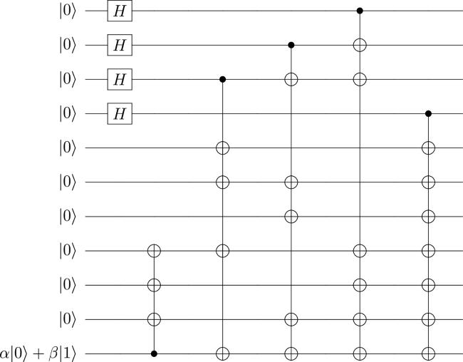
For every quantum state ∣$\Psi$⟩, we can show the corresponding quantum circuit diagram. For example, consider the quantum state ∣$\Psi$⟩ = α∣$\Psi$0,4⟩ + β∣$\Psi$1,4⟩, as shown in figure 1.
Figure 1. Quantum circuit diagram for generating ∣$\Psi$⟩ state.

4. Application of quantum information masking

Quantum information masking forms the basis for quantum secret sharing, where legitimate participants can recover the original quantum state through collaboration, while unauthorized ones cannot. Therefore, Alice encodes the original information α∣0⟩ + β∣1⟩ into a multipartite quantum state ∣$\Psi$⟩ = α∣$\Psi$0⟩ + β∣$\Psi$1⟩, and then distributes each particle of ∣$\Psi$⟩ to each participant. We term the stage of recovering the secret with minimal participants as the secret recovery phase. In this section, to highlight the applicability of the quantum states, we will explore how to recover the secret using the state ∣$\Psi$⟩ = α∣$\Psi$0,4⟩ + β∣$\Psi$1,4⟩ as shown in Example 1.
Alice prepares the quantum state ∣$\Psi$⟩ and sends each particle to each participant via a decoy photon sequence. These participants can be denoted by P1, P2, …, P11. During the recovery process, we omitted the coefficient of ∣$\Psi$0,4⟩ and ∣$\Psi$1,4⟩ as they do not affect the final result.
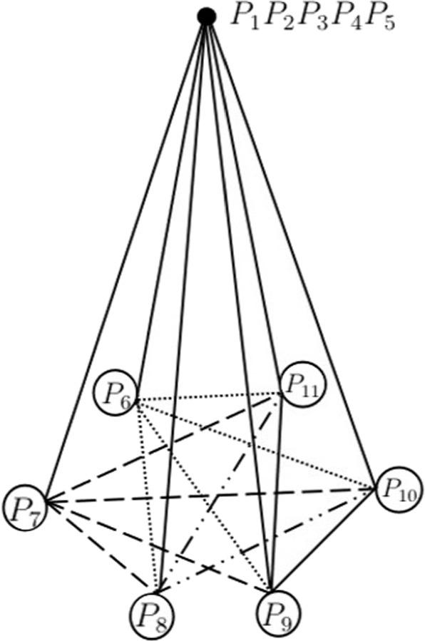
In addition, we consider the structure of the legitimate participants as shown in figure 2, where the structure can be represented as
$\begin{eqnarray}\begin{array}{l}{\rm{\Gamma }}=\{\{{P}_{1},{P}_{2},{P}_{3},{P}_{4},{P}_{5},{P}_{6},{P}_{8}\},\\ \quad \{{P}_{1},{P}_{2},{P}_{3},{P}_{4},{P}_{5},{P}_{6},{P}_{9}\},\\ \quad \{{P}_{1},{P}_{2},{P}_{3},{P}_{4},{P}_{5},{P}_{6},{P}_{10}\},\\ \quad \{{P}_{1},{P}_{2},{P}_{3},{P}_{4},{P}_{5},{P}_{6},{P}_{11}\},\\ \quad \{{P}_{1},{P}_{2},{P}_{3},{P}_{4},{P}_{5},{P}_{7},{P}_{8}\},\\ \quad \{{P}_{1},{P}_{2},{P}_{3},{P}_{4},{P}_{5},{P}_{7},{P}_{9}\},\\ \quad \{{P}_{1},{P}_{2},{P}_{3},{P}_{4},{P}_{5},{P}_{7},{P}_{10}\},\\ \quad \{{P}_{1},{P}_{2},{P}_{3},{P}_{4},{P}_{5},{P}_{7},{P}_{11}\},\\ \quad \{{P}_{1},{P}_{2},{P}_{3},{P}_{4},{P}_{5},{P}_{8},{P}_{10}\},\\ \quad \{{P}_{1},{P}_{2},{P}_{3},{P}_{4},{P}_{5},{P}_{8},{P}_{11}\},\\ \quad \{{P}_{1},{P}_{2},{P}_{3},{P}_{4},{P}_{5},{P}_{9},{P}_{10}\},\\ \quad \{{P}_{1},{P}_{2},{P}_{3},{P}_{4},{P}_{5},{P}_{9},{P}_{11}\}\}.\end{array}\end{eqnarray}$
Figure 2. Schematic of seven participants collaborating to recover secrets, where each triangle formed by connecting vertex P1P2P3P4P5 with any two endpoints of the edges below represents a valid secret recovery set.
In figure 2, we present all sets of participants that can recover secrets. Furthermore, we take the set P1, P2, P3, P4, P5, P6, P8 as an example. Other situations can be similarly analyzed.
Step 1. The participant P4 carries out several measurements on his particle in ∣$\Psi$⟩ under the basis of {∣0⟩, ∣1⟩}. At the same time, the remaining participants can get the following collapse states on their own particles.
(1) If the measurement by P4 is ∣0⟩, then the quantum state ∣$\Psi$⟩ can collapse to $| {\tilde{\phi }}_{0}\rangle $, where $| {\tilde{\phi }}_{0}\rangle $ is denoted by
$\begin{eqnarray}\begin{array}{rcl}|{\tilde{\phi }}_{0}\rangle & = & {\left(\alpha \left|000\rangle \,+\,\beta |111\right\rangle \right)}_{123}|00000000\rangle \\ & & \,+\,{\left(\alpha \left|101\rangle \,+\,\beta |010\right\rangle \right)}_{123}|01010101\rangle \\ & & \,+\,{\left(\alpha \left|011\rangle \,+\,\beta |100\right\rangle \right)}_{123}|00110011\rangle \\ & & \,+\,{\left(\alpha \left|110\rangle \,+\,\beta |001\right\rangle \right)}_{123}|01100110\rangle \\ & & \,+\,{\left(\alpha \left|111\rangle \,+\,\beta |000\right\rangle \right)}_{123}|00001111\rangle \\ & & \,+\,{\left(\alpha \left|010\rangle +\beta |101\right\rangle \right)}_{123}|01011010\rangle \\ & & \,+\,{\left(\alpha \left|100\rangle \,+\,\beta |011\right\rangle \right)}_{123}|00111100\rangle \\ & & \,+\,{\left(\alpha \left|001\rangle \,+\,\beta |110\right\rangle \right)}_{123}|01101001\rangle .\end{array}\end{eqnarray}$
(2) If the measurement by P4 is ∣1⟩, then the quantum state ∣$\Psi$⟩ can collapse to $| {\tilde{\phi }}_{1}\rangle $, where $| {\tilde{\phi }}_{1}\rangle $ is denoted by
$\begin{eqnarray}\begin{array}{rcl}|{\tilde{\phi }}_{1}\rangle & \,=\, & {\left(\alpha \left|000\rangle \,+\,\beta |111\right\rangle \right)}_{123}|11111111\rangle \\ & & \,+\,{\left(\alpha \left|101\rangle \,+\,\beta |010\right\rangle \right)}_{123}|10101010\rangle \\ & & \,+\,{\left(\alpha \left|011\rangle \,+\,\beta |100\right\rangle \right)}_{123}|11001100\rangle \\ & & \,+\,{\left(\alpha \left|110\rangle \,+\,\beta |001\right\rangle \right)}_{123}|10011001\rangle \\ & & \,+\,{\left(\alpha \left|111\rangle \,+\,\beta |000\right\rangle \right)}_{123}|11110000\rangle \\ & & \,+\,{\left(\alpha \left|010\rangle \,+\,\beta |101\right\rangle \right)}_{123}|10100101\rangle \\ & & \,+\,{\left(\alpha \left|100\rangle \,+\,\beta |011\right\rangle \right)}_{123}|11000011\rangle \\ & & \,+\,{\left(\alpha \left|001\rangle \,+\,\beta |110\right\rangle \right)}_{123}|10010110\rangle .\end{array}\end{eqnarray}$
Step 2. The participant P5 measures the quantum state $| {\tilde{\phi }}_{0}\rangle $ or $| {\tilde{\phi }}_{1}\rangle $ with a computational basis {∣0⟩, ∣1⟩}. Then, he can obtain four cases, namely, four quantum states are collapsed into
$\begin{eqnarray}\begin{array}{rcl}|{\tilde{\phi }}_{00}\rangle & = & {\left(\alpha \left|000\rangle \,+\,\beta |111\right\rangle \right)}_{123}|00000000\rangle \\ & & \,+\,{\left(\alpha \left|011\rangle \,+\,\beta |100\right\rangle \right)}_{123}|00110011\rangle \\ & & \,+\,{\left(\alpha \left|111\rangle \,+\,\beta |000\right\rangle \right)}_{123}|00001111\rangle \\ & & \,+\,{\left(\alpha \left|100\rangle \,+\,\beta |011\right\rangle \right)}_{123}|00111100\rangle ,\end{array}\end{eqnarray}$
$\begin{eqnarray}\begin{array}{rcl}|{\tilde{\phi }}_{01}\rangle & = & {\left(\alpha \left|101\rangle \,+\,\beta |010\right\rangle \right)}_{123}|01010101\rangle \\ & & \,+\,{\left(\alpha \left|110\rangle \,+\,\beta |001\right\rangle \right)}_{123}|01100110\rangle \\ & & \,+\,{\left(\alpha \left|010\rangle \,+\,\beta |101\right\rangle \right)}_{123}|01011010\rangle \\ & & \,+\,{\left(\alpha \left|001\rangle \,+\,\beta |110\right\rangle \right)}_{123}|01101001\rangle ,\end{array}\end{eqnarray}$
$\begin{eqnarray}\begin{array}{rcl}|{\tilde{\phi }}_{10}\rangle & = & {\left(\alpha \left|101\rangle \,+\,\beta |010\right\rangle \right)}_{123}|10101010\rangle \\ & & \,+\,{\left(\alpha \left|110\rangle \,+\,\beta |001\right\rangle \right)}_{123}|10011001\rangle \\ & & \,+\,{\left(\alpha \left|010\rangle \,+\,\beta |101\right\rangle \right)}_{123}|10100101\rangle \\ & & \,+\,{\left(\alpha \left|001\rangle \,+\,\beta |110\right\rangle \right)}_{123}|10010110\rangle ,\end{array}\end{eqnarray}$
$\begin{eqnarray}\begin{array}{rcl}|{\tilde{\phi }}_{11}\rangle & = & {\left(\alpha \left|000\rangle \,+\,\beta |111\right\rangle \right)}_{123}|11111111\rangle \\ & & \,+\,{\left(\alpha \left|011\rangle \,+\,\beta |100\right\rangle \right)}_{123}|11001100\rangle \\ & & \,+\,{\left(\alpha \left|111\rangle \,+\,\beta |000\right\rangle \right)}_{123}|11110000\rangle \\ & & \,+\,{\left(\alpha \left|100\rangle \,+\,\beta |011\right\rangle \right)}_{123}|11000011\rangle .\end{array}\end{eqnarray}$
Step 3. P6 and P8 use {∣00⟩, ∣01⟩, ∣10⟩, ∣11⟩} to measure their particles of $| {\tilde{\phi }}_{00}\rangle $, $| {\tilde{\phi }}_{01}\rangle $, $| {\tilde{\phi }}_{10}\rangle $ or $| {\tilde{\phi }}_{11}\rangle $. These states obtained after measurement are as follows,
$\begin{eqnarray}\begin{array}{rcl}| {\tilde{\phi }}_{0000}\rangle & = & {\left(\alpha | 000\rangle +\beta | 111\rangle \right)}_{123}| 00000000\rangle ,\\ | {\tilde{\phi }}_{0001}\rangle & = & {\left(\alpha | 111\rangle +\beta | 000\rangle \right)}_{123}| 00001111\rangle ,\\ | {\tilde{\phi }}_{0010}\rangle & = & {\left(\alpha | 011\rangle +\beta | 100\rangle \right)}_{123}| 00110011\rangle ,\\ | {\tilde{\phi }}_{0011}\rangle & = & {\left(\alpha | 100\rangle +\beta | 011\rangle \right)}_{123}| 00111100\rangle ,\\ | {\tilde{\phi }}_{0100}\rangle & = & {\left(\alpha | 101\rangle +\beta | 010\rangle \right)}_{123}| 01010101\rangle ,\\ | {\tilde{\phi }}_{0101}\rangle & = & {\left(\alpha | 010\rangle +\beta | 101\rangle \right)}_{123}| 01011010\rangle ,\\ | {\tilde{\phi }}_{0110}\rangle & = & {\left(\alpha | 110\rangle +\beta | 001\rangle \right)}_{123}| 01100110\rangle ,\\ | {\tilde{\phi }}_{0111}\rangle & = & {\left(\alpha | 001\rangle +\beta | 110\rangle \right)}_{123}| 01101001\rangle ,\\ | {\tilde{\phi }}_{1000}\rangle & = & {\left(\alpha | 001\rangle +\beta | 110\rangle \right)}_{123}| 10010110\rangle ,\\ | {\tilde{\phi }}_{1001}\rangle & = & {\left(\alpha | 110\rangle +\beta | 001\rangle \right)}_{123}| 10011001\rangle ,\\ | {\tilde{\phi }}_{1010}\rangle & = & {\left(\alpha | 010\rangle +\beta | 101\rangle \right)}_{123}| 10100101\rangle ,\\ | {\tilde{\phi }}_{1011}\rangle & = & {\left(\alpha | 101\rangle +\beta | 010\rangle \right)}_{123}| 10101010\rangle ,\\ | {\tilde{\phi }}_{1100}\rangle & = & {\left(\alpha | 100\rangle +\beta | 011\rangle \right)}_{123}| 11000011\rangle ,\\ | {\tilde{\phi }}_{1101}\rangle & = & {\left(\alpha | 011\rangle +\beta | 100\rangle \right)}_{123}| 11001100\rangle ,\\ | {\tilde{\phi }}_{1110}\rangle & = & {\left(\alpha | 111\rangle +\beta | 000\rangle \right)}_{123}| 11110000\rangle ,\\ | {\tilde{\phi }}_{1111}\rangle & = & {\left(\alpha | 000\rangle +\beta | 111\rangle \right)}_{123}| 11111111\rangle .\end{array}\end{eqnarray}$
Step 4. These participants, {P1, P2, P3}, cooperate to use a Controlled-NOT gate on their particles with the first qubit as the control and the second and third qubits as target bits. Then, the above states in equation (38) yields the following states,
$\begin{eqnarray}\begin{array}{rcl}| {\phi }_{0000}\rangle & = & {\left(\alpha | 0\rangle +\beta | 1\rangle \right)}_{1}| 0000000000\rangle ,\\ | {\phi }_{0001}\rangle & = & {\left(\alpha | 1\rangle +\beta | 0\rangle \right)}_{1}| 0000001111\rangle ,\\ | {\phi }_{0010}\rangle & = & {\left(\alpha | 0\rangle +\beta | 1\rangle \right)}_{1}| 1100110011\rangle ,\\ | {\phi }_{0011}\rangle & = & {\left(\alpha | 1\rangle +\beta | 0\rangle \right)}_{1}| 1100111100\rangle ,\\ | {\phi }_{0100}\rangle & = & {\left(\alpha | 1\rangle +\beta | 0\rangle \right)}_{1}| 1001010101\rangle ,\\ | {\phi }_{0101}\rangle & = & {\left(\alpha | 0\rangle +\beta | 1\rangle \right)}_{1}| 1001011010\rangle ,\\ | {\phi }_{0110}\rangle & = & {\left(\alpha | 1\rangle +\beta | 0\rangle \right)}_{1}| 0101100110\rangle ,\\ | {\phi }_{0111}\rangle & = & {\left(\alpha | 0\rangle +\beta | 1\rangle \right)}_{1}| 0101101001\rangle ,\\ | {\phi }_{1000}\rangle & = & {\left(\alpha | 0\rangle +\beta | 1\rangle \right)}_{1}| 0110010110\rangle ,\\ | {\phi }_{1001}\rangle & = & {\left(\alpha | 1\rangle +\beta | 0\rangle \right)}_{1}| 0110011001\rangle ,\\ | {\phi }_{1010}\rangle & = & {\left(\alpha | 0\rangle +\beta | 1\rangle \right)}_{1}| 1010100101\rangle ,\\ | {\phi }_{1011}\rangle & = & {\left(\alpha | 1\rangle +\beta | 0\rangle \right)}_{1}| 1010101010\rangle ,\\ | {\phi }_{1100}\rangle & = & {\left(\alpha | 1\rangle +\beta | 0\rangle \right)}_{1}| 1111000011\rangle ,\\ | {\phi }_{1101}\rangle & = & {\left(\alpha | 0\rangle +\beta | 1\rangle \right)}_{1}| 1111001100\rangle ,\\ | {\phi }_{1110}\rangle & = & {\left(\alpha | 1\rangle +\beta | 0\rangle \right)}_{1}| 0011110000\rangle ,\\ | {\phi }_{1111}\rangle & = & {\left(\alpha | 0\rangle +\beta | 1\rangle \right)}_{1}| 0011111111\rangle .\end{array}\end{eqnarray}$
Step 5. According to the measurements of the four participants P4, P5, P6, P8, P1 performs the following operations, as shown in table 1. Therefore, P1 can recover the original quantum state α∣0⟩ + β∣1⟩.
Table 1. The operations to recover the secret executed by P1P2P3P4P5P6P8, where I represents the identical operation and X represents the bit flip operation.
Measurement result Collapsed states States after using a Operations
by P4P5P6P8 after measurement CNOT gate with P1P2P3 performed by P1
∣0000⟩ $| {\tilde{\phi }}_{0000}\rangle $ φ0000 I
∣0001⟩ $| {\tilde{\phi }}_{0001}\rangle $ φ0001 X
∣0010⟩ $| {\tilde{\phi }}_{0010}\rangle $ φ0010 I
∣0011⟩ $| {\tilde{\phi }}_{0011}\rangle $ φ0011 X
∣0100⟩ $| {\tilde{\phi }}_{0100}\rangle $ φ0100 X
∣0101⟩ $| {\tilde{\phi }}_{0101}\rangle $ φ0101 I
∣0110⟩ $| {\tilde{\phi }}_{0110}\rangle $ φ0110 X
∣0111⟩ $| {\tilde{\phi }}_{0111}\rangle $ φ0111 I
∣1000⟩ $| {\tilde{\phi }}_{1000}\rangle $ φ1000 I
∣1001⟩ $| {\tilde{\phi }}_{1001}\rangle $ φ1001 X
∣1010⟩ $| {\tilde{\phi }}_{1010}\rangle $ φ1010 I
∣1011⟩ $| {\tilde{\phi }}_{1011}\rangle $ φ1011 X
∣1100⟩ $| {\tilde{\phi }}_{1100}\rangle $ φ1100 X
∣1101⟩ $| {\tilde{\phi }}_{1101}\rangle $ φ1101 I
∣1110⟩ $| {\tilde{\phi }}_{1110}\rangle $ φ1110 X
∣1111⟩ $| {\tilde{\phi }}_{1111}\rangle $ φ1111 I

5. Conclusion

In this paper, we introduced a framework for 1-uniform quantum information masking in multipartite systems, facilitated by the application of a Fourier matrix. Furthermore, we constructed an orthogonal array utilizing a specialized Fourier matrix, which we then leverage to develop a methodology for the implementation of 2-uniform quantum information masking. Subsequently, we generated two 2-uniform states ∣$\Psi$0⟩ and ∣$\Psi$1⟩ based on the corresponding orthogonal array. Next, we proceeded to demonstrate that a quantum state ∣$\Psi$⟩ = α∣$\Psi$0⟩ + β∣$\Psi$1⟩ can mask the quantum state into multipartite systems. Moreover, if the number of qubits for ∣$\Psi$0⟩ and ∣$\Psi$1⟩ decreased sequentially from left to right, and the count N satisfies the condition 2n−1 + 3 ≤ N ≤ 2n − 1, ∣$\Psi$⟩ could also achieve 2-uniform masking. To illustrate our method, we presented a quantum circuit diagram for generating ∣$\Psi$⟩ when n = 4. Finally, to prove that our scheme can be applied to quantum secret sharing, we also provided a specific application of 2-uniform quantum information masking.

Appendix: The proof of theorem 3.

Firstly, when n = 3 and $N={2}^{3}-1$, the following 2-uniform quantum state can be obtained from the orthogonal array of equation (14),

$\begin{eqnarray}\begin{array}{rcl}|1\rangle \mapsto |{{\rm{\Psi }}}_{1}^{{2}^{3}}\rangle & = & \displaystyle \frac{1}{\sqrt{{2}^{3}}}(|1111111\rangle \,+\,|0101010\rangle \\ & & \,+\,|1001100\rangle \,+\,|0011001\rangle \\ & & \,+\,|1110000\rangle \,+\,|0100101\rangle \\ & & \,+\,|1000011\rangle \,+\,|0010110\rangle )\\ & = & \displaystyle \sum _{i=1}^{{2}^{3}}\displaystyle \frac{1}{\sqrt{{2}^{3}}}|{\gamma }_{i}\rangle .\end{array}\end{eqnarray}$

Based on Lemma 2, we have $\langle {\gamma }_{i}| {\gamma }_{j}\rangle =0,\,i,\,j\in \{1,2,\ldots ,{2}^{3}\},\,i\ne j$. Furthermore, another 2-uniform quantum state can be obtained, namely,

$\begin{eqnarray}\begin{array}{rcl}|0\rangle \mapsto |{{\rm{\Psi }}}_{0}^{{2}^{3}}\rangle & = & {X}^{\left.\otimes ({2}^{3}-1\right)}|{{\rm{\Psi }}}_{1}^{{2}^{3}}\rangle \\ & = & \displaystyle \frac{1}{\sqrt{{2}^{3}}}\left(\left|0000000\rangle \,+\,|1010101\right\rangle \right.\\ & & \,+\,|0110011\rangle \,+\,|1100110\rangle \\ & & \,+\,|0001111\rangle \,+\,|1011010\rangle \\ & & \left.+\left|0111100\rangle \,+\,|1101001\right\rangle \right)\\ & = & \displaystyle \sum _{i=1}^{{2}^{3}}\displaystyle \frac{1}{\sqrt{{2}^{3}}}|{\bar{\gamma }}_{i}\rangle .\end{array}\end{eqnarray}$
Similarly, it is easy to get $\langle {\overline{\gamma }}_{i}| {\overline{\gamma }}_{j}\rangle =0,\,i,\,j\in \{1,2,\ldots ,{2}^{3}\}$ and $i\ne j$.

Utilizing the inherent characteristics of the orthogonal array, the first two bits of each quantum state can be extracted and obtained, namely,

$\begin{eqnarray}\begin{array}{rcl}|{{\rm{\Psi }}}_{1}^{{2}^{3}}\rangle & = & \displaystyle \frac{1}{\sqrt{{2}^{3}}}(|11\rangle |11111\rangle \,+\,|01\rangle |01010\rangle \\ & & \,+\,|10\rangle |01100\rangle \,+\,|00\rangle |11001\rangle \\ & & \,+\,|11\rangle |10000\rangle \,+\,|01\rangle |00101\rangle \\ & & \,+\,|10\rangle |00011\rangle \,+\,|00\rangle |10110\rangle )\\ & \triangleq & \displaystyle \frac{1}{\sqrt{{2}^{3}}}(|11\rangle (|{\delta }_{1}\rangle \,+\,|{\delta }_{2}\rangle )+|01\rangle (|{\delta }_{3}\rangle \,+\,|{\delta }_{4}\rangle )\\ & & \,+\,|10\rangle (|{\delta }_{5}\rangle \,+\,|{\delta }_{6}\rangle )+|11\rangle (|{\delta }_{7}\rangle \,+\,|{\delta }_{8}\rangle )),\end{array}\end{eqnarray}$
$\begin{eqnarray}\begin{array}{rcl}| {{\rm{\Psi }}}_{0}^{{2}^{3}}\rangle & = & \displaystyle \frac{1}{\sqrt{{2}^{3}}}(| 00\rangle | 00000\rangle +| 10\rangle | 10101\rangle \\ & & +| 01\rangle | 10011\rangle +| 11\rangle | 00110\rangle \\ & & +| 00\rangle | 01111\rangle +| 10\rangle | 11010\rangle \\ & & +| 01\rangle | 11100\rangle +| 11\rangle | 01001\rangle )\\ & \triangleq & \displaystyle \frac{1}{\sqrt{{2}^{3}}}(| 00\rangle (| {\overline{\delta }}_{1}\rangle +| {\overline{\delta }}_{2}\rangle )+| 10\rangle (| {\overline{\delta }}_{3}\rangle +| {\overline{\delta }}_{4}\rangle )\\ & & +| 01\rangle (| {\overline{\delta }}_{5}\rangle +| {\overline{\delta }}_{6}\rangle )+| 00\rangle (| {\overline{\delta }}_{7}\rangle +| {\overline{\delta }}_{8}\rangle )),\end{array}\end{eqnarray}$
where $\langle {\delta }_{i}| {\delta }_{j}\rangle =0,$ $\langle {\overline{\delta }}_{i}| {\overline{\delta }}_{j}\rangle =0,$ $\langle {\delta }_{i}| {\overline{\delta }}_{i}\rangle =0,$ $\langle {\overline{\delta }}_{i}| {\delta }_{i}\rangle \,=0,$ $i,\,j\in \{1,2,\ldots ,{2}^{3}\},\,i\ne j$.

Therefore, for $| {\rm{\Psi }}\rangle =\alpha | {{\rm{\Psi }}}_{0}^{{2}^{3}}\rangle +\beta | {{\rm{\Psi }}}_{1}^{{2}^{3}}\rangle $($| \alpha {| }^{2}+| \beta {| }^{2}=1$), tracing out the $3,4,\cdots ,({2}^{3}-1)$ qubits, we find the reduced density operator of the first and the second qubits,

$\begin{eqnarray}{\rho }_{12}={\mathrm{Tr}}_{34\cdots ({2}^{3}-1)}\left[| {\rm{\Psi }}\rangle \langle {\rm{\Psi }}| \right]=\displaystyle \frac{{I}_{4}}{4}.\end{eqnarray}$
From the arbitrariness of orthogonal arrays, it can be inferred that
$\begin{eqnarray}{\rho }_{{ij}}=\displaystyle \frac{{I}_{4}}{4},\,\,\,\,\,i,\,j\in \{1,2,\ldots ,{2}^{3}-1\},\,i\ne j.\end{eqnarray}$
Thus, when n = 3, all the quantum states $\alpha | 0\rangle +\beta | 1\rangle $ can be 2-uniformly masked into $| {\rm{\Psi }}\rangle =\alpha | {{\rm{\Psi }}}_{0}^{{2}^{3}}\rangle +\beta | {{\rm{\Psi }}}_{1}^{{2}^{3}}\rangle $.

Next, consider when n = 4 and $N={2}^{4}-1$. According to the general formula of the Hadamard matrix,

$\begin{eqnarray}{H}_{{2}^{4}}={H}_{{2}^{3}}\otimes {H}_{2}=\left(\begin{array}{rr}{H}_{{2}^{3}} & {H}_{{2}^{3}}\\ {H}_{{2}^{3}} & -{H}_{{2}^{3}}\end{array}\right).\end{eqnarray}$
It is easy to obtain that
$\begin{eqnarray}\mathrm{OA}({2}^{4},{2}^{4}-1,2,2)=\left(\begin{array}{ccc}{\gamma }_{1} & 1 & {\gamma }_{1}\\ {\gamma }_{2} & 1 & {\gamma }_{2}\\ \vdots & \vdots & \vdots \\ {\gamma }_{{2}^{3}} & 1 & {\gamma }_{{2}^{3}}\\ {\gamma }_{1} & 0 & {\overline{\gamma }}_{1}\\ {\gamma }_{2} & 0 & {\overline{\gamma }}_{2}\\ \vdots & \vdots & \vdots \\ {\gamma }_{{2}^{3}} & 0 & {\overline{\gamma }}_{{2}^{3}}\end{array}\right).\end{eqnarray}$
Accordingly, two 2-uniform quantum states can be gained, denoted as
$\begin{eqnarray}| {{\rm{\Psi }}}_{1}^{{2}^{4}}\rangle =\displaystyle \frac{1}{\sqrt{{2}^{4}}}\displaystyle \sum _{i=1}^{{2}^{3}}| {\gamma }_{i}\rangle (| 1\rangle | {\gamma }_{i}\rangle +| 0\rangle | {\overline{\gamma }}_{i}\rangle ),\end{eqnarray}$
$\begin{eqnarray}| {{\rm{\Psi }}}_{0}^{{2}^{4}}\rangle ={X}^{\otimes ({2}^{4}-1)}| {{\rm{\Psi }}}_{1}^{{2}^{4}}\rangle =\displaystyle \frac{1}{\sqrt{{2}^{4}}}\displaystyle \sum _{i=1}^{{2}^{3}}| {\overline{\gamma }}_{i}\rangle (| 0\rangle | {\overline{\gamma }}_{i}\rangle +| 1\rangle | {\gamma }_{i}\rangle ).\end{eqnarray}$
As a consequence,
$\begin{eqnarray}\begin{array}{rcl}| {\rm{\Psi }}\rangle & = & \alpha | {{\rm{\Psi }}}_{0}^{{2}^{4}}\rangle +\beta | {{\rm{\Psi }}}_{1}^{{2}^{4}}\rangle \\ & = & \displaystyle \frac{1}{\sqrt{{2}^{4}}}\displaystyle \sum _{i=1}^{{2}^{3}}\left[\alpha (| {\overline{\gamma }}_{i}\rangle | 0\rangle | {\overline{\gamma }}_{i}\rangle +| {\overline{\gamma }}_{i}\rangle | 1\rangle | {\gamma }_{i}\rangle )\right.\\ & & \left.+\beta (| {\gamma }_{i}\rangle | 1\rangle | {\gamma }_{i}\rangle +| {\gamma }_{i}\rangle | 0\rangle | {\overline{\gamma }}_{i}\rangle )\right],\end{array}\end{eqnarray}$
where $| {\overline{\gamma }}_{i}\rangle | 0\rangle | {\overline{\gamma }}_{i}\rangle $, $| {\overline{\gamma }}_{i}\rangle | 1\rangle | {\gamma }_{i}\rangle $, $| {\gamma }_{i}\rangle | 1\rangle | {\gamma }_{i}\rangle $ and $| {\gamma }_{i}\rangle | 0\rangle | {\overline{\gamma }}_{i}\rangle $ are quantum states generated by each row of $\mathrm{OA}({2}^{4},{2}^{4}-1,2,2)$.

Based on the basic properties of orthogonal array, the first two qubits of each quantum state in $| {\rm{\Psi }}\rangle $ can be extracted, resulting in the following form

$\begin{eqnarray}\begin{array}{rcl}| {\rm{\Psi }}\rangle & = & \displaystyle \frac{1}{\sqrt{{2}^{4}}}\left[\alpha (| 00\rangle (| {\zeta }_{1}\rangle +| {\zeta }_{2}\rangle +| {\zeta }_{3}\rangle +| {\zeta }_{4}\rangle )\right.\\ & & +| 10\rangle (| {\zeta }_{5}\rangle +| {\zeta }_{6}\rangle +| {\zeta }_{7}\rangle +| {\zeta }_{8}\rangle )\\ & & +| 01\rangle (| {\zeta }_{9}\rangle +| {\zeta }_{10}\rangle +| {\zeta }_{11}\rangle +| {\zeta }_{12}\rangle )\\ & & +| 11\rangle (| {\zeta }_{13}\rangle +| {\zeta }_{14}\rangle +| {\zeta }_{15}\rangle +| {\zeta }_{16}\rangle ))\\ & & +\beta (| 11\rangle (| {\overline{\zeta }}_{1}\rangle +| {\overline{\zeta }}_{2}\rangle +| {\overline{\zeta }}_{3}\rangle +| {\overline{\zeta }}_{4}\rangle )\\ & & +| 01\rangle (| {\overline{\zeta }}_{5}\rangle +| {\overline{\zeta }}_{6}\rangle +| {\overline{\zeta }}_{7}\rangle +| {\overline{\zeta }}_{8}\rangle )\\ & & +| 10\rangle (| {\overline{\zeta }}_{9}\rangle +| {\overline{\zeta }}_{10}\rangle +| {\overline{\zeta }}_{11}\rangle +| {\overline{\zeta }}_{12}\rangle )\\ & & \left.+| 00\rangle (| {\overline{\zeta }}_{13}\rangle +| {\overline{\zeta }}_{14}\rangle +| {\overline{\zeta }}_{15}\rangle +| {\overline{\zeta }}_{16}\rangle ))\right],\end{array}\end{eqnarray}$
where $\langle {\zeta }_{i}| {\zeta }_{j}\rangle =0,$ $\langle {\overline{\zeta }}_{i}| {\overline{\zeta }}_{j}\rangle =0,$ $\langle {\zeta }_{i}| {\overline{\zeta }}_{i}\rangle =0,$ $\langle {\overline{\zeta }}_{i}| {\zeta }_{i}\rangle =0,$ $i,\,j\in \{1,2,\ldots ,{2}^{4}\}$ and $i\ne j$.

It is easy to calculate that

$\begin{eqnarray}{\rho }_{12}={\mathrm{Tr}}_{34\cdots ({2}^{4}-1)}\left[| {\rm{\Psi }}\rangle \langle {\rm{\Psi }}| \right]=\displaystyle \frac{{I}_{4}}{4}.\end{eqnarray}$
And due to the arbitrariness of the basic properties of orthogonal arrays, there is
$\begin{eqnarray}{\rho }_{{ij}}=\displaystyle \frac{{I}_{4}}{4},\,\,\,\,\,i,\,j\in \{1,2,\ldots ,{2}^{4}-1\},\,i\ne j.\end{eqnarray}$
As a result, when n = 4, all the quantum states $\alpha | 0\rangle +\beta | 1\rangle $ can be 2-uniformly masked into $| {\rm{\Psi }}\rangle =\alpha | {{\rm{\Psi }}}_{0}^{{2}^{4}}\rangle +\beta | {{\rm{\Psi }}}_{1}^{{2}^{4}}\rangle $.

Suppose that n = m and $N={2}^{m}-1$, $\alpha | 0\rangle +\beta | 1\rangle $ can also be 2-uniformly masked into $| {\rm{\Psi }}\rangle =\alpha | {{\rm{\Psi }}}_{0}^{{2}^{m}}\rangle +\beta | {{\rm{\Psi }}}_{1}^{{2}^{m}}\rangle $. Below, we will focus solely on the case where $n=m+1$ and $N={2}^{m+1}-1$.

For convenience, the orthogonal array corresponding to ${H}_{{2}^{m}}$ can be denoted as

$\begin{eqnarray}\mathrm{OA}({2}^{m},{2}^{m}-1,2,2)=\left(\begin{array}{c}{\gamma }_{1}\\ {\gamma }_{2}\\ \vdots \\ {\gamma }_{{2}^{m}}\end{array}\right),\end{eqnarray}$
where $\langle {\gamma }_{i}| {\gamma }_{j}\rangle =0,$ $i,\,j\in \{1,2,\ldots ,{2}^{m}\}$ and $i\ne j$.

Therefore, the orthogonal array corresponding to ${H}_{{2}^{m+1}}$ can be represented as

$\begin{eqnarray}\mathrm{OA}({2}^{m+1},{2}^{m+1}-1,2,2)=\left(\begin{array}{ccc}{\gamma }_{1} & 1 & {\gamma }_{1}\\ {\gamma }_{2} & 1 & {\gamma }_{2}\\ \vdots & \vdots & \vdots \\ {\gamma }_{{2}^{m}} & 1 & {\gamma }_{{2}^{m}}\\ {\gamma }_{1} & 0 & {\overline{\gamma }}_{1}\\ {\gamma }_{2} & 0 & {\overline{\gamma }}_{2}\\ \vdots & \vdots & \vdots \\ {\gamma }_{{2}^{m}} & 0 & {\overline{\gamma }}_{{2}^{m}}\end{array}\right).\end{eqnarray}$
So, the generated 2-uniform states are
$\begin{eqnarray}| {{\rm{\Psi }}}_{1}^{{2}^{m+1}}\rangle =\displaystyle \frac{1}{\sqrt{{2}^{m+1}}}\displaystyle \sum _{i=1}^{{2}^{m}}| {\gamma }_{i}\rangle (| 1\rangle | {\gamma }_{i}\rangle +| 0\rangle | {\overline{\gamma }}_{i}\rangle ),\end{eqnarray}$
$\begin{eqnarray}\begin{array}{rcl}| {{\rm{\Psi }}}_{0}^{{2}^{m+1}}\rangle & = & {X}^{\otimes ({2}^{m+1}-1)}| {{\rm{\Psi }}}_{1}^{{2}^{m+1}}\rangle \\ & = & \displaystyle \frac{1}{\sqrt{{2}^{m+1}}}\displaystyle \sum _{i=1}^{{2}^{m}}| {\overline{\gamma }}_{i}\rangle (| 0\rangle | {\overline{\gamma }}_{i}\rangle +| 1\rangle | {\gamma }_{i}\rangle ).\end{array}\end{eqnarray}$
As a consequence,
$\begin{eqnarray}\begin{array}{rcl}| {\rm{\Psi }}\rangle & = & \alpha | {{\rm{\Psi }}}_{0}^{{2}^{m+1}}\rangle +\beta | {{\rm{\Psi }}}_{1}^{{2}^{m+1}}\rangle \\ & = & \displaystyle \frac{1}{\sqrt{{2}^{m+1}}}\displaystyle \sum _{i=1}^{{2}^{m}}\left[\alpha (| {\overline{\gamma }}_{i}\rangle | 0\rangle | {\overline{\gamma }}_{i}\rangle +| {\overline{\gamma }}_{i}\rangle | 1\rangle | {\gamma }_{i}\rangle )\right.\\ & & \left.+\beta (| {\gamma }_{i}\rangle | 1\rangle | {\gamma }_{i}\rangle +| {\gamma }_{i}\rangle | 0\rangle | {\overline{\gamma }}_{i}\rangle )\right],\end{array}\end{eqnarray}$
where $| {\overline{\gamma }}_{i}\rangle | 0\rangle | {\overline{\gamma }}_{i}\rangle ,$ $| {\overline{\gamma }}_{i}\rangle | 1\rangle | {\gamma }_{i}\rangle ,$ $| {\gamma }_{i}\rangle | 1\rangle | {\gamma }_{i}\rangle $ and $| {\gamma }_{i}\rangle | 0\rangle | {\overline{\gamma }}_{i}\rangle $ are quantum states generated by each row of $\mathrm{OA}({2}^{m+1},{2}^{m+1}-1,2,2)$.

Therefore, by Lemma 2, we know that they are pairwise orthogonal. In addition, based on the properties of orthogonal array, the first two qubits of each quantum state in $| {\rm{\Psi }}\rangle $ can be extracted, as follow,

$\begin{eqnarray}\begin{array}{rcl}| {\rm{\Psi }}\rangle & = & \displaystyle \frac{1}{\sqrt{{2}^{m+1}}}\left[\displaystyle \sum _{i=1}^{{2}^{m-1}}(\alpha | 00\rangle | {\xi }_{i}\rangle +\beta | 11\rangle | {\overline{\xi }}_{i}\rangle )\right.\\ & & +\displaystyle \sum _{i={2}^{m-1}+1}^{{2}^{m}}(\alpha | 10\rangle | {\xi }_{i}\rangle +\beta | 01\rangle | {\overline{\xi }}_{i}\rangle )\\ & & +\displaystyle \sum _{i={2}^{m}+1}^{{2}^{m}+{2}^{m-1}}(\alpha | 01\rangle | {\xi }_{i}\rangle +\beta | 10\rangle | {\overline{\xi }}_{i}\rangle )\\ & & \left.+\displaystyle \sum _{i={2}^{m}+{2}^{m-1}+1}^{{2}^{m+1}}(\alpha | 11\rangle | {\xi }_{i}\rangle +\beta | 00\rangle | {\overline{\xi }}_{i}\rangle )\right],\end{array}\end{eqnarray}$
where $\langle {\xi }_{i}| {\xi }_{j}\rangle =0,$ $\langle {\overline{\xi }}_{i}| {\overline{\xi }}_{j}\rangle =0,$ $\langle {\xi }_{i}| {\overline{\xi }}_{i}\rangle =0,$ $\langle {\overline{\xi }}_{i}| {\xi }_{i}\rangle \,=0,$ $i,\,j\in \{1,2,\ldots ,{2}^{m+1}\},i\ne j$.

We calculate that

$\begin{eqnarray}{\rho }_{12}={\mathrm{Tr}}_{34\cdots ({2}^{m+1}-1)}\left[| {\rm{\Psi }}\rangle \langle {\rm{\Psi }}| \right]=\displaystyle \frac{{I}_{4}}{4}.\end{eqnarray}$
Since the arbitrariness of the orthogonal array, it is easy to verify that
$\begin{eqnarray}{\rho }_{{ij}}=\displaystyle \frac{{I}_{4}}{4},\,\,\,\,\,i,\,j\in \{1,2,\ldots ,{2}^{m+1}-1\},\,i\ne j.\end{eqnarray}$
Thus, all the quantum states $\alpha | 0\rangle +\beta | 1\rangle $ can be 2-uniformly masked into $| {\rm{\Psi }}\rangle =\alpha | {{\rm{\Psi }}}_{0}\rangle +\beta | {{\rm{\Psi }}}_{1}\rangle $. This completes the proof.

We want to express our gratitude to anonymous referees for their valuable and constructive comments. This work is supported by the National Natural Science Foundation of China under Grant No. 12301590 and the Natural Science Foundation of Hebei Province under Grant No. A2022210002.

1
Wootters W K, Zurek W H 1982 A single quantum cannot be cloned Nature 299 802

DOI

2
Dieks D 1982 Overlap and distinguishability of quantum states Phys. Lett. A 92 271

DOI

3
Yuen H P 1986 Amplification of quantum states and noiseless photon amplifiers Phys. Lett. A 113 405

DOI

4
Pati A K, Braunstein S L 2000 Impossibility of deleting an unknown quantunm state Nature 404 164

DOI

5
Braunstein S L, Pati A K 2007 Quantum information cannot be completely hidden in correlations: implications for the black-hole information paradox Phys. Rev. Lett. 98 080502

DOI

6
Girling M, Cîrstoiu C, Jennings D 2024 Simple formulation of no-cloning and no-hiding that admits efficient and robust verification Phys. Rev. Res. 6 023090

DOI

7
Kalev A, Hen I 2008 No-broadcasting theorem and its classical counterpart Phys. Rev. Lett. 100 210502

DOI

8
Heinosaari T, Jenčová A, Plávala M 2023 Dispensing of quantum information beyond nobroadcasting theorem is it possible to broadcast anything genuinely quantum J. Phys. A: Math. Theor. 56 135301

DOI

9
Horodecki R, Horodecki P, Horodecki M, Horodecki K 2009 Quantum entanglement Rev. Mod. Phys. 81 865

DOI

10
Grünenfelder F 2023 Fast single-photon detectors and real-time key distillation enable high secret-key-rate quantum key distribution systems Nat. Photon. 17 422 426

DOI

11
Bouwmeester D 1997 Experimental quantum teleportation Nature 390 575

DOI

12
Hermans L N 2022 Qubit teleportation between nonneighbouring nodes in a quantum network Nature 605 663 668

DOI

13
Hillery M, Bužek V, Berthiaume A 1999 Quantum secret sharing Phys. Rev. A 59 1829

DOI

14
Senthoor K, Sarvepalli P K 2022 Theory of communication efficient quantum secret sharing IEEE Trans. Inf. Theory 68 3164 3186

DOI

15
Singh P, Chakrabarty I 2024 Controlled state reconstruction and quantum secret sharing Phys. Rev. A 109 032406

DOI

16
Bai C M, Zhang S J, Liu L 2022 Quantum secret sharing based on quantum information masking Quantum Inf. Process. 21 377

DOI

17
Modi K, Pati A K, Sen(De) A, Sen U 2018 Masking quantum information is impossible Phys. Rev. Lett. 120 230501

DOI

18
Li M S, Wang Y L 2018 Masking quantum information in multipartite scenario Phys. Rev. A 98 062306

DOI

19
Wang M Y, Zhang S J, Bai C M, Liu L 2022 The masking condition for the quantum state in two-dimensional Hilbert space Commun. Theor. Phys. 74 115101

DOI

20
Wang Q, Zhang S J, Bai C M, Liu L 2022 The condition of masking quantum qutric ststes Laser Phys. Lett. 19 115201

DOI

21
Li B 2019 Deterministic versus probabilistic quantum information masking Phys. Rev. A 99 052343

DOI

22
Lie S H, Jeong H 2020 Randomness cost of masking quantum information and the information conservation law Phys. Rev. A 101 052322

DOI

23
Liu Z H 2021 Photonic implementation of quantum information masking Phys. Rev. Lett. 126 170505

DOI

24
Du Y 2021 Masking quantum information encoded in pure and mixed states Int. J. Theor. Phys. 60 2380 2399

DOI

25
Li M S, Modi K 2020 Probabilistic and approximate masking of quantum information Phys. Rev. A 102 022418

DOI

26
Zhu H J 2021 Hiding and masking quantum information in complex and real quantum mechanics Phys. Rev. Res. 3 033176

DOI

27
Shi F, Li M S, Chen L, Zhang X 2021 k-uniform quantum information masking Phys. Rev. A 104 032601

DOI

28
Zhang S M, Wang M H, Zhou B 2023 Quantifying the information distribution of quantum information masking Quantum Inf. Process. 22 284

DOI

29
Shang W M, Fan X Y, Zhang F L, Chen J L 2023 Quantum information masking of an arbitrary unknown state can be realized in the multipartite lower-dimensional systems Phys. Scr. 98 035102

DOI

30
Shen Y, Zhang F L, Chen Y Z, Zhou C C 2023 Masking quantum information in the Kitaev Abelian anyons Phys. A 612 128495

DOI

31
Wang M Y 2024 Masking quantum information in multipartite systems based on generator matrices Laser Phys. 34 055203

DOI

32
Shen Y 2024 Anyonic quantum multipartite maskers in the Kitaev model Phys. Rev. A 109 032421

DOI

33
Arnaud L, Cerf N J 2013 Exploring pure quantum states with maximally mixed reductions Phys. Rev. A 87 012319

DOI

34
Goyeneche D, Zyczkowski K 2014 Genuinely multipartite entangled states and orthogonal arrays Phys. Rev. A 90 022316

DOI

35
Rao C R 1946 Hypercubes of strength'd'leading to confounded designs in factorial experiments Bull. Calcutta Math. Soc. 38 67 78

36
Hedayat A S, Sloane N J A, Stufken J 2012 Orthogonal Arrays: Theory and Applications Springer

37
Cheng C S 1980 Orthogonal arrays with variable numbers of symbols Ann. Stat. 8 447 453

DOI

Outlines

/