


1. Introduction
Quantum metrology is of importance to multiple areas of scientific research, including gravitational wave detection [1], biological sensing [2], atomic clocks [3], magnetometry [4, 5], and so on. The task is to estimate unknown parameters encoded in quantum systems. The achievable estimation precision realized in classical physics is subject to the shot noise limit (SNL) $1/\sqrt{N}$, where N is the number of resources employed in the measurements. If one adopts nonclassical resources such as squeezing and entanglement, the achievable estimation precision can beat the SNL [6, 7]. Especially, for some states such as Greenberger–Horne–Zeilinger states, the estimation precision can reach the Heisenberg limit (HL) 1/N [8, 9]. However, in real experiments, the system of interest inevitably couples to its surrounding environment, which is known as an open quantum system (OQS). The dynamics of an OQS are characterized by decoherence, which inevitably deteriorates the estimation precision.
The achievable precision under the noisy environment has been investigated previously. For frequency estimation under a Markovian pure dephasing noise, the estimation precision returns to the SNL [10]. For a relaxation noise, the estimation precision scales asymptotically as N−5/6 [11]. Some estimation protocols under the non-Markovian environment have also been investigated. It was predicted in the Ramsey spectroscopy that the precision can reach N−3/4 [12], which was argued to be a consequence of the quantum Zeno effect at short time scales. This prediction was recently confirmed in a real experiment [13]. Afterwards, a novel limit on the attainable precision in frequency estimation was derived by [14], which holds for all forms of phase covariant uncorrelated noise. In recent years, Bai et al proposed that if the probe and environment formed a bound state [15–17], the estimation precision can asymptotically recover to the ideal case in a long-time condition, where the dissipation was exactly studied by non-Markovian dynamic evolution. Tan et al have found that using coherent spin states can reach a 1/(Nt) scale estimation precision of the spectral density for super-Ohmic environment [18]. Those studies highlight the advantages of non-Markovian quantum metrology.
To improve the estimation precision, researchers have proposed using proper controls to mitigate the harmfulness of noises [19–22]. Recently, some researchers focused on finding optimal controls based on different algorithms [23–28] to enhance the metrology performance. A particularly efficient method is gradient-based algorithms such as Gradient Ascent Pulse Engineering [23–25]. Other methods based on the Pontryagin Maximum Principle [26, 27] are another option. In those works, they assume that the system is dissipated in the Markovian environment. Under the premise of the Born–Markov approximation, the reduced system dynamics can be described by a Lindblad master equation [29, 30]. However, such approximation is valid only for a memoryless environment. In many practical scenarios with long-time environmental correlation, Markovian approximation is no longer valid, leading to distinct non-Markovian behavior [12–17, 31–34]. Therefore, finding the optimal control under non-Markovian environments becomes a subject of interest.
In this work, we tackle the problem of finding the optimal control under an arbitrary non-Markovian bosonic environment, where the environment is characterized by its spectral density. By introducing a pseudomode model, the original environment can be replaced by few dissipated pseudomode harmonic oscillators with proper parameters. The evolution of the system's density matrix can be equivalently and accurately described by a Lindblad master equation, which provides a simple description for an OQS. With the help of this pseudomode model, we derivate the gradient of quantum Fisher information (QFI), which allows us to use the gradient ascent algorithm to find the optimal control making QFI maximal. To show the effectiveness of our method, we consider the frequency estimation of a spin with multi-axis control under Lorentz and Ohmic spectral environments. Our results demonstrate a significant enhancement in QFI, which shows the effectiveness of our method in optimizing quantum metrology protocols under a non-Markovian environment.
2. Accurate description of the non-Markovian dissipation model
As illustrated in figure 1(a), we consider a system coupling to a bosonic environment. The total Hamiltonian is given by
$\begin{eqnarray}{\hat{H}}_{\mathrm{tot}}={\hat{H}}_{{\rm{s}}}+{\hat{H}}_{\mathrm{env}}+\hat{V},\end{eqnarray}$
where ${\hat{H}}_{{\rm{s}}}$, ${\hat{H}}_{\mathrm{env}}$, $\hat{V}$ are the Hamiltonians of the system, environment and interaction, respectively. The environment Hamiltonian reads $\begin{eqnarray}{\hat{H}}_{\mathrm{env}}=\displaystyle \sum _{k}{\omega }_{k}{\hat{b}}_{k}^{\dagger }{\hat{b}}_{k},\end{eqnarray}$
where bk is kth boson mode's annihilation operator of the environment, with the characteristic frequency ωk. Initially, the environment is in a thermal state with a temperature of T. We consider the interaction Hamiltonian $\begin{eqnarray}\hat{V}=\hat{S}\otimes \hat{B},\end{eqnarray}$
where $\hat{S}$ is the operator of system and $\hat{B}={\sum }_{k}{g}_{k}{\hat{b}}_{k}+{g}_{k}^{* }{\hat{b}}_{k}^{\dagger }$ is the operator of environment.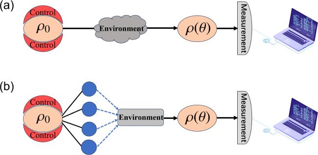
Figure 1. Two equivalent open quantum system models used for noisy quantum metrology. Under the influence of control and environment, the system evolves to the final state ρ(θ) encoded by an unknown parameter θ. (a) The original open quantum system model. The system couples to a non-Markovian bosonic environment characterized by a certain spectrum. (b) An equivalent pseudomode model. The system couples to few pseudomode harmonic oscillators, but the oscillators are collectively dissipated in a Markovian bosonic environment. The two models are equivalent if their correlation functions are equal. |
The effects of the system-environment interaction are characterized by the correlation function (COF), namely
$\begin{eqnarray}C(t)\equiv \langle \hat{B}(t)\hat{B}\rangle ,\end{eqnarray}$
where $\hat{B}(t)\equiv {{\rm{e}}}^{{\rm{i}}{\hat{H}}_{\mathrm{env}}t}\hat{B}{{\rm{e}}}^{-{\rm{i}}{\hat{H}}_{\mathrm{env}}t}$ and ⟨⋯⟩ denotes the expectation value with respect to the initial state of the environment. Defining the spectral density $J(\omega )\equiv {\sum }_{k}{\left|{g}_{k}\right|}^{2}\delta \left(\omega -{\omega }_{k}\right)$ in continuum limit, the COF is given by [35] $\begin{eqnarray}C(t)=\int {\rm{d}}\omega J(\omega )\left[\coth \left(\displaystyle \frac{\beta \omega }{2}\right)\cos (\omega t)-{\rm{i}}\,\sin (\omega t)\right],\end{eqnarray}$
where β = 1/(KbT) and Kb is the Boltzmann constant. If the system's initial state $\rho \left(0\right)$ and the operator $\hat{S}$ are given, the reduced density matrix of the system is fully dominated by the COF [36–40], which is the characteristic of Gaussian bosonic environment.The original model can also be exactly simulated by an equivalent pseudomode model shown in figure 1(b). The system couples to M pseudomode harmonic oscillators, but the oscillators are collectively dissipated in a pseudo environment. The total Hamiltonian of the pseudomode model is given by9 ) is given by
$\begin{eqnarray}{\hat{H}}_{\mathrm{pse}}={\hat{H}}_{{\rm{s}}}+\hat{S}\otimes {\hat{B}}_{\mathrm{pse}}+{\hat{H}}_{{\rm{B}},\mathrm{pse}},\end{eqnarray}$
with $\begin{eqnarray}{\hat{B}}_{\mathrm{pse}}=\displaystyle \sum _{j=1}^{M}{\eta }_{j}{\hat{c}}_{j}^{\dagger }+{\eta }_{j}^{* }{\hat{c}}_{j},\end{eqnarray}$
and $\begin{eqnarray}\begin{array}{rcl}{\hat{H}}_{{\rm{B}},\mathrm{pse}} & = & \displaystyle \sum _{j=1}^{M}{{\rm{\Omega }}}_{j}{\hat{c}}_{j}^{\dagger }{\hat{c}}_{j}+\displaystyle \sum _{k}{\omega }_{k}{\hat{b}}_{k}^{\dagger }{\hat{b}}_{k}\\ & & +\displaystyle \sum _{k}\displaystyle \sum _{j=1}^{M}{g}_{j,k}{\hat{b}}_{k}{\hat{c}}_{j}^{\dagger }+{g}_{j,k}^{* }{\hat{b}}_{k}^{\dagger }{\hat{c}}_{j}.\end{array}\end{eqnarray}$
Here, ηj denotes the interaction strength between the system and jth harmonic oscillator, gj,k denotes the coupling strength between the jth harmonic oscillator and kth boson mode of the pseudo environment. For convenience, we consider gj,k = μj, i.e., the pseudo environment is Markovian, which gives a simplified description of the original model. If we regard the system and harmonic oscillators as a whole, it undergoes dissipation within a Markovian environment, which can be described by a Lindblad master equation [40] $\begin{eqnarray}\displaystyle \frac{\partial {\rho }_{\mathrm{sc}}}{\partial t}=-{\rm{i}}\left[\hat{H},{\rho }_{\mathrm{sc}}\right]+{ \mathcal D }\left[\displaystyle \sum _{j=1}^{M}{\mu }_{j}{\hat{c}}_{j}\right]{\rho }_{\mathrm{sc}}\equiv { \mathcal L }{\rho }_{\mathrm{sc}},\end{eqnarray}$
where ${ \mathcal L }$ is the Liouvillian superoperator and $\begin{eqnarray}\hat{H}={\hat{H}}_{s}+\displaystyle \sum _{j=1}^{M}{{\rm{\Omega }}}_{j}{\hat{c}}_{j}^{\dagger }{\hat{c}}_{j}+\hat{S}\otimes {\hat{B}}_{\mathrm{pse}},\end{eqnarray}$
$\begin{eqnarray}{ \mathcal D }[\hat{A}]{\rho }_{\mathrm{sc}}\equiv \hat{A}{\rho }_{\mathrm{sc}}{\hat{A}}^{\dagger }-\displaystyle \frac{{\rho }_{\mathrm{sc}}{\hat{A}}^{\dagger }\hat{A}+{\hat{A}}^{\dagger }\hat{A}{\rho }_{\mathrm{sc}}}{2}.\end{eqnarray}$
Using the matrix representation of the superoperator [41], the solution of equation ( $\begin{eqnarray}{\rho }_{\mathrm{sc}}\left(t\right)={{\rm{e}}}^{{ \mathcal L }t}{\rho }_{\mathrm{sc}}\left(0\right),\end{eqnarray}$
with the initial state ${\rho }_{\mathrm{sc}}\left(0\right)={\rho }_{{\rm{s}}}\left(0\right)\otimes {\rho }_{\mathrm{vac}}^{\otimes M}$, where ${\rho }_{{\rm{s}}}\left(0\right)$ is the initial state of system and ρvac is the vacuum state of the harmonic oscillator. Note that ρsc is the total density matrix of the system and the pseudomode oscillators, the reduced density matrix of the system is obtained by tracing out the pseudomode oscillators, i.e., $\begin{eqnarray}\rho \left(t\right)={\mathrm{Tr}}_{{\rm{c}}}\left[{\rho }_{\mathrm{sc}}\left(t\right)\right].\end{eqnarray}$
The two models in figures 1(a) and (b) are equivalent if their COFs are equal. In other words, given a non-Markovian model shown in figure 1(a), we can always find an equivalent pseudomode model shown in figure 1(b) with appropriate parameters (Ωj, μj, ηj). The procedures of determining the parameters (Ωj, μj, ηj) are shown in appendix A . In the following, we will use the pseudomode model to exactly simulate a certain non-Markovian environment and find the optimal control to improve the performance of quantum metrology.
3. Quantum metrology theory with optimal control
Given the system's reduced density matrix ρ(t, θ) encoding an unknown parameter θ, the estimation precision about θ obeys the quantum Cramér–Rao inequality [9]9 )–(13 ). After getting ρ(t) and its derivative, one can calculate ${F}_{Q}\left(t\right)$.
$\begin{eqnarray}\delta \theta \geqslant \displaystyle \frac{1}{\sqrt{{F}_{Q}}},\end{eqnarray}$
where $\begin{eqnarray}{F}_{Q}=\mathrm{Tr}\left(\rho {l}^{2}\right)\end{eqnarray}$
is the QFI and l is the symmetric logarithmic derivative determined by $\begin{eqnarray}\displaystyle \frac{\partial \rho }{\partial \theta }=\displaystyle \frac{\rho l+l\rho }{2}.\end{eqnarray}$
Considering a non-Markovian model shown in figure 1(a) with a certain environmental spectrum, we can design an equivalent pseudomode model with proper parameters (Ωj, μj, ηj) shown in figure 1(b). Thus, the system's reduced density matrix ρ(t) can be solved by equations (To improve the performance of metrology, we consider a controlled Hamiltonian10 ), $\{{\hat{H}}_{k}\}$ is a set of control applied to the system, and ${f}_{k}\left(t\right)$ is the control functions to be optimized. For such a time-dependent Hamiltonian, the dynamical evolution can be described by the Lindblad master equation18 ) is accurate and does not involve any approximations. The above equation can be solved by the time discretization method. Specifically, we set a time range $t\in \left[0,T\right]$ and separate the range into N segments, which gives a succession of ${f}_{k}\left({t}_{i}\right)$ and ${{ \mathcal L }}_{i}\equiv { \mathcal L }\left({t}_{i}\right)$ with i = 1, ⋯ ,N. The size of each segment is Δt = T/N. Next, performing the iterations15 )–(16 ), we can calculate the symmetric logarithmic derivative $l\left(T\right)$ and ${F}_{Q}\left(T\right)$.
$\begin{eqnarray}\hat{H}\left(t\right)=\hat{H}+\displaystyle \sum _{k}{f}_{k}\left(t\right){\hat{H}}_{k},\end{eqnarray}$
where $\hat{H}$ is the free Hamiltonian given by equation ( $\begin{eqnarray}\displaystyle \frac{\partial {\rho }_{\mathrm{sc}}}{\partial t}=-{\rm{i}}\left[\hat{H}\left(t\right),{\rho }_{\mathrm{sc}}\right]+{ \mathcal D }\left[\displaystyle \sum _{j=1}^{M}{\mu }_{j}{\hat{c}}_{j}\right]{\rho }_{\mathrm{sc}}\equiv { \mathcal L }\left(t\right){\rho }_{\mathrm{sc}}.\end{eqnarray}$
We emphasize that equation ( $\begin{eqnarray}{\rho }_{\mathrm{sc}}\left({t}_{i+1}\right)={{\rm{e}}}^{{{ \mathcal L }}_{i}{\rm{\Delta }}t}{\rho }_{\mathrm{sc}}\left({t}_{i}\right),\end{eqnarray}$
and $\begin{eqnarray}\displaystyle \frac{\partial {\rho }_{\mathrm{sc}}({t}_{i+1})}{\partial \theta }=\displaystyle \frac{\partial {{\rm{e}}}^{{{ \mathcal L }}_{i}{\rm{\Delta }}t}}{\partial \theta }{\rho }_{\mathrm{sc}}\left({t}_{i}\right)+{{\rm{e}}}^{{{ \mathcal L }}_{i}{\rm{\Delta }}t}\displaystyle \frac{\partial {\rho }_{\mathrm{sc}}\left({t}_{i}\right)}{\partial \theta },\end{eqnarray}$
for i = 1 to N, we can obtain ${\rho }_{\mathrm{sc}}\left({t}_{N+1}\right)$ and $\partial {\rho }_{\mathrm{sc}}\left({t}_{N+1}\right)/\partial \theta $. Tracing out the pseudomodes, we obtain $\rho \left(T\right)\,={\mathrm{Tr}}_{{\rm{c}}}\left[{\rho }_{\mathrm{sc}}\left({t}_{N+1}\right)\right]$ and $\partial \rho \left(T\right)/\partial \theta ={\mathrm{Tr}}_{{\rm{c}}}\left[\partial {\rho }_{\mathrm{sc}}\left({t}_{N+1}\right)/\partial \theta \right]$. Using equations (Due to ${F}_{Q}\left(T\right)$ being highly related to the control fk(ti), we need to find the optimal fk(ti) making ${F}_{Q}\left(T\right)$ maximal. A powerful method is the gradient ascent method, which requires the gradient of ${F}_{Q}\left(T\right)$ with respect to fk(ti). We regard ${f}_{k}\left({t}_{i}\right)$ as variables to be optimized and calculate the corresponding gradients (details are shown in appendix B )22 ), $\partial {F}_{Q}\left(T\right)/\partial {f}_{k}^{\left(n\right)}\left({t}_{i}\right)$ should be recalculated by equation (21 ). If ${F}_{Q}\left(T\right)$ converges after a sufficient number of iteration steps, we terminate the iteration. Concurrently, the optimal control is obtained.
$\begin{eqnarray}\displaystyle \frac{\partial {F}_{Q}\left(T\right)}{\partial {f}_{k}\left({t}_{i}\right)}={\mathrm{Tr}}_{{\rm{s}}}\left[2l{\mathrm{Tr}}_{{\rm{c}}}\displaystyle \frac{{\partial }^{2}{\rho }_{\mathrm{sc}}\left(T\right)}{\partial {f}_{k}\left({t}_{i}\right)\partial \theta }-{l}^{2}{\mathrm{Tr}}_{{\rm{c}}}\displaystyle \frac{\partial {\rho }_{\mathrm{sc}}\left(T\right)}{\partial {f}_{k}\left({t}_{i}\right)}\right].\end{eqnarray}$
Next, we set the initial values of ${f}_{k}\left({t}_{i}\right)\ $ to zero and perform a gradient-based iteration $\begin{eqnarray}{f}_{k}^{\left(n+1\right)}\left({t}_{i}\right)={f}_{k}^{\left(n\right)}\left({t}_{i}\right)+\epsilon \displaystyle \frac{\partial {F}_{Q}\left(T\right)}{\partial {f}_{k}^{\left(n\right)}\left({t}_{i}\right)},\end{eqnarray}$
where ${f}_{k}^{\left(n\right)}\left({t}_{i}\right)$ denotes the control function fk at time ti and at the nth iteration, ε is a proper positive number (i.e., the so called learning rate). For each step in equation (4. Example: frequency estimation of a spin with optimal two-axis control
As an example, we now consider a 1/2-spin dissipated in a bosonic environment with the spin Hamiltonian1 ) and equation (3 ) with $\hat{S}={\hat{\sigma }}_{z}/2$. Given the environmental temperature T and the spectral density function J(ω), the COF can be calculated by equation (5 ). If we take the initial state $\left(\left|\uparrow \right\rangle +\left|\downarrow \right\rangle \right)/\sqrt{2}$, the exact solution of the reduced density matrix is given by [35]16 ), one can calculate the QFI [12]
$\begin{eqnarray}{\hat{H}}_{{\rm{s}}}=\displaystyle \frac{{\omega }_{0}}{2}{\hat{\sigma }}_{z},\end{eqnarray}$
where ω0 is the frequency to be estimated and ${\hat{\sigma }}_{z}$ is the Pauli-z operator. The total Hamiltonian and interaction Hamiltonian are given by equation ( $\begin{eqnarray}\begin{array}{rcl}\rho (t) & = & \displaystyle \frac{\left|\uparrow \right\rangle \left\langle \,\uparrow \,\right|+\left|\downarrow \right\rangle \left\langle \,\downarrow \,\right|}{2}\\ & + & \displaystyle \frac{{{\rm{e}}}^{-\gamma \left(t\right)}}{2}\left({{\rm{e}}}^{-{\rm{i}}{\omega }_{0}t}\left|\uparrow \right\rangle \left\langle \,\downarrow \,\right|+{{\rm{e}}}^{{\rm{i}}{\omega }_{0}t}\left|\downarrow \right\rangle \left\langle \,\uparrow \,\right|\right),\end{array}\end{eqnarray}$
where $\begin{eqnarray}\gamma \left(t\right)=\int {\rm{d}}\omega J(\omega )\coth (\displaystyle \frac{\beta \omega }{2})\displaystyle \frac{1-\cos (\omega t)}{{\omega }^{2}}.\end{eqnarray}$
The estimation precision of the frequency ω0 is bounded by $1/\sqrt{{F}_{Q}}$. Using equations (15) and ( $\begin{eqnarray}{F}_{Q}={t}^{2}{{\rm{e}}}^{-2\gamma \left(t\right)}.\end{eqnarray}$
To improve the estimation precision of ω0, we consider a two-axis control strategy with a controlled Hamiltonian18 ) with
$\begin{eqnarray}\hat{H}\left(t\right)=\hat{H}+{f}_{x}\left(t\right){\hat{\sigma }}_{x}+{f}_{y}\left(t\right){\hat{\sigma }}_{y}.\end{eqnarray}$
The dynamical evolution is described by equation ( $\begin{eqnarray}\hat{H}={\hat{H}}_{s}+\displaystyle \sum _{j=1}^{M}{{\rm{\Omega }}}_{j}{\hat{c}}_{j}^{\dagger }{\hat{c}}_{j}+\displaystyle \frac{{\hat{\sigma }}_{z}}{2}\otimes \displaystyle \sum _{j=1}^{M}\left({\eta }_{j}{\hat{c}}_{j}^{\dagger }+{\eta }_{j}^{* }{\hat{c}}_{j}\right),\end{eqnarray}$
where the values of Ωj, μj, ηj depend on the specific environmental spectrum. In the subsequent discussion, we will examine two types of environmental spectra and demonstrate the optimal control that maximizes the QFI.4.1. Lorentz spectral environment
For a Lorentz spectral environment, the spectral density function is given by26 ) and (30 ), which is shown in figure 2(a). The red dashed line is the numerical result, obtained by our pseudomode method (equations (9 ) and (15 )). One can find that the numerical result coincides with the analytical one, which verifies the validity of our pseudomode method.
$\begin{eqnarray}J(\omega )=\displaystyle \frac{{\chi }^{2}}{\pi }\displaystyle \frac{{\rm{\Gamma }}}{{\left(\omega -{\omega }_{c}\right)}^{2}+{{\rm{\Gamma }}}^{2}},\end{eqnarray}$
where χ is the coupling strength and Γ is the spectral width. At zero temperature, we have $\begin{eqnarray}\gamma \left(t\right)={\int }_{-\infty }^{\infty }{\rm{d}}\omega J(\omega )\displaystyle \frac{1-\cos (\omega t)}{{\omega }^{2}}.\end{eqnarray}$
For the non-control case, the QFI can be calculated by equations (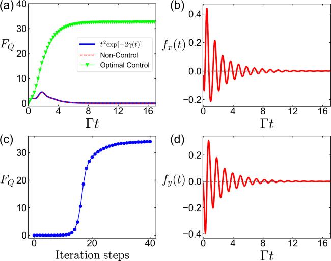
Figure 2. The QFI and optimal control under a Lorentz spectral environment. (a) The comparison of the QFI between the non-control case (blue line) and the optimal control case (green triangles). The blue line is the analytical result of the QFI given by equation ( |
For the control case, we need to exactly calculate the dynamical evolution under the Lorentz spectral environment. We utilize the pseudomode model depicted in figure 1(b), which comprises only one pseudomode harmonic oscillator with a frequency Ω1 = ωc, a dissipation rate ${\mu }_{1}=\sqrt{2{\rm{\Gamma }}}$ and a coupling strength η1 = χ. To obtain the optimal control, we use the gradient ascent algorithm shown in equations (21 ) and (22 ). As shown in figure 2(c), the QFI gradually converges after 40 iterations. The optimal control functions ${f}_{x}\left(t\right)$ and ${f}_{y}\left(t\right)$ are shown in figures 2(b) and (d). The black lines are the initial values of ${f}_{x}\left(t\right)$ and ${f}_{y}\left(t\right)$, which are taken as zero. Using optimal ${f}_{x}\left(t\right)$ and ${f}_{y}\left(t\right)$, we show the comparison of controlled QFI and non-controlled QFI in figure 2(a), which indicates a significant improvement in QFI.
At the long-time limit, we observe that the QFI no longer exhibits any increase. This is because the system evolves into a steady state under the influence of control. In figures 3(a)–(c), we plot the expectation values of ${\hat{\sigma }}_{x}$, ${\hat{\sigma }}_{y}$ and ${\hat{\sigma }}_{z}$, which indicate that the off-diagonal elements of the density matrix are gradually decaying to zero. The presence of the control field not only decelerates the decay of off-diagonal elements, but also encodes the information about ω0 into the diagonal elements. When the steady state is reached, the information about ω0 is only encoded in diagonal elements, which explains why the QFI remains constant. Even if the control is removed, the QFI remains unchanged (see figure 3(d)).
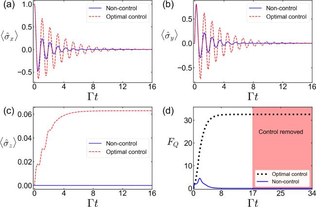
Figure 3. (a)-(c) The expectation values of ${\hat{\sigma }}_{x}$, ${\hat{\sigma }}_{y}$, ${\hat{\sigma }}_{z}$ for both the non-control and optimal control cases. (d) The comparison of QFI between non-control and optimal control protocol, with the control field being applied within the time region where Γt < 17. The control field is removed when Γt ≥ 17, as indicated by the pink region. |
4.2. Ohmic spectral environment
The Ohmic spectral environment is widely considered for electron transfer dynamics [42] or biomolecular complexes [43], as well as Josephson junctions qubits [44]. The spectral density function is given by $J(\omega )=\chi \omega {{\rm{e}}}^{-\omega /{\omega }_{c}}$ (ω > 0), where χ is the coupling strength and ωc is the cut-off frequency. At zero temperature, we have
$\begin{eqnarray}\gamma \left(t\right)=\displaystyle \frac{\chi }{2}\mathrm{ln}\ \left(1+{\omega }_{c}^{2}{t}^{2}\right).\end{eqnarray}$
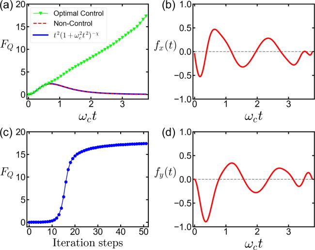
Under the short time condition, we have $\gamma \left(t\right)\approx \tfrac{\chi }{2}{\omega }_{c}^{2}{t}^{2}\propto {t}^{2}$, which indicates a quantum Zeno effect [12]. The QFI of non-control case is given by $\begin{eqnarray}{F}_{Q}={t}^{2}{{\rm{e}}}^{-2\gamma \left(t\right)}=\displaystyle \frac{{t}^{2}}{{\left(1+{\omega }_{c}^{2}{t}^{2}\right)}^{\chi }}.\end{eqnarray}$
To find the optimal control, we need to exactly simulate the dynamical evolution under Ohmic spectral environment. Different to the Lorentz spectral case, we use the pseudomode model shown in figure 1(b) containing 3 pseudomode harmonic oscillators with the frequencies (Ω1, Ω2, Ω3), the dissipation rates (μ1,μ2, μ3 ) and interaction strengths (η1, η2, η3). These pseudomode parameters can be determined by the procedures shown in appendix A . In figure 4, we show the comparison of COF between the original model (solid lines) and the pseudomode model (dashed lines), given by equation (5 ) and equation (A2 ). The coincidence of COFs indicates that the two models are nearly equivalent. If one expects a higher accuracy, it is possible to increase the number of pseudomode harmonic oscillators, albeit at the cost of increasing the computational cost.
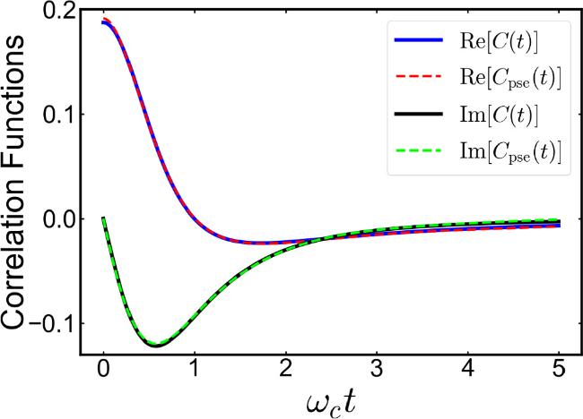
Figure 4. The real part and the imaginary part of the COF for the original Ohmic spectral model and the pseudomode model. We take the coupling strength χ = 3 and the cut-off frequency ωc = 0.25. The pseudomode parameters: (Ω1,Ω2,Ω3) = (0.241, 1.267 31, −0.203), (μ1,μ2,μ3) = (0.5648, 1.1465, 0.8938) and (η1, η2, η3) = (0.0289+0.3711i, −0.0177 − 0.2272i, 0.002 28+0.02931i). |
As demonstrated in figure 5(a), the effectiveness of the pseudomode method can be confirmed by the agreement between the QFI values in the non-control scenario. Using the gradient ascent algorithm, we derive the optimal control strategy under an Ohmic environment. The iterative process is shown in figure 5(c), and the optimal control functions ${f}_{x}\left(t\right)$ and ${f}_{y}\left(t\right)$ are shown in figures 5(b) and (d). The comparison of the controlled QFI and the non-controlled QFI are shown in figure 5(a), which indicates a significant improvement in QFI.
Figure 5. The QFI and optimal control under the Ohmic spectral environment. (a) The comparison of QFI between non-control case (blue line) and optimal control case (green triangles). The blue line is the analytical result of QFI given by equation ( |
5. Conclusion
In summary, we have used a pseudomode model method to find the optimal control to improve the performance of the quantum metrology under an arbitrary non-Markovian bosonic environment. The original model is replaced by a pseudomode model which contains few harmonic oscillators with proper parameters dissipated in one Markovian environment. The time evolution is equivalently described by a time-dependent Lindblad master equation. By exactly solving the dynamics, we calculate the gradient of the QFI and use the gradient ascent algorithm to find the optimal control.
To demonstrate its validity, we examine the frequency estimation of a spin system with pure dephasing under two distinct non-Markovian environments. To simulate the evolution of the spin, we introduce one pseudomode harmonic oscillator for the case of a Lorentz spectral environment and three pseudomode harmonic oscillators for the case of an Ohmic spectral environment. For the non-control case, numerical results of the QFI align with analytical findings. By maximizing the QFI at a fixed evolution time, we numerically obtain the optimal multi-axis control, which yields a significant enhancement in the QFI compared to the non-control scenario.