


1. Introduction
Light gets deflected when it travels near a massive object due to the interaction of the object and gravitational field with light. Therefore, gravitational lensing is a phenomenon where each large object acts like a lens. Gravitational lensing is split into weak and strong fields based on the deflection angle of light. A light beam experiences a weak deflection limit when it travels far from the photon sphere, and a large deflection limit when it travels close to the photon sphere. After that, relativistic pictures may be created by rotating the lens one or more times. There is no way to form a picture since light rays entering the photon sphere are trapped in the lens' gravitational field. An effective observational technique for studying black holes (BHs) at the centers of galaxies is gravitational lensing. A survey of several gravitational lensing techniques and observational prospects is given in [1–4]. Because of the divergence of curvature, cosmological and BH solutions that result in singularities in General Relativity (GR) are essential subjects. Gravitational lensing is the name given to the phenomenon where light is deflected by gravity. A highly useful technique for studying the Universe, galaxies, and dark matter is gravitational lensing. Several investigations on gravitational lensing for BHs, wormholes, and various other objects have been performed since Eddington's initial observation. Gravitational lensing is a really interesting topic [5–24]. It provides details on the pictured source, the lensing object, and the intervening large-scale geometry of the Universe when the source, lens, and observer are at cosmic distances from one another. The deflection angle permits the strong deflection limit, a logarithmic approximation that makes it possible to analytically determine the locations, magnifications, and time delays of the relativistic pictures. First introduced for the Schwarzschild BH [25], this approximate approach was then expanded to the Reissner–Nordström spacetime [26], and finally, it was generalized to any spherically symmetric and asymptotically flat geometry [27, 28].
The most often applied technique for figuring out the weak deflection angle is probably the Gauss–Bonnet theorem (GBT), which was initially introduced in [29]. Since then, several BH models exhibiting asymptotic behavior have proved the GBT to be incredibly useful in estimating the weak deflection angle [30–32]. Other significant research on the investigation of the weak deflection angle also exists, including those on dark matter, phantom matter, and fundamental energy [33–36]. The possibility of exotic matter or energy gravitationally lensing matter, potentially deviating from a well-known equation of state, is also investigated [37]. In terms of the asymptotic form of the GBT, it appears difficult to calculate the weak deflection angle for non-asymptotic spacetimes. The computation was recently made possible by taking into account the finite distances between the source and the receiver in an enhanced analysis found in [38]. However, the GBT and finite-distance coincide with the difficult task of evaluating integrals, which in turn make up the orbit equation. This method is useful in the strong gravitational lensing zone [39, 40] as well, independent of whether or not the spacetime is axially symmetric [41].
The study of gravitational lensing and the BH are the most efficient astrophysical techniques for probing the strong-field properties of gravity and may provide an important test of modified theories of gravity in strong-field regimes. Due to the significant improvements in modern observational capabilities, there has been a great deal of interest focused on the gravitational deflection of light by revolving BHs [42–46]. Numerous theories of gravity have examined the geometry of BHs with different parameters [47, 48]. Examining the impact of a plasma background on a BH is a fascinating subject. The evidence for the occurrence of BHs at galaxy centers has made the study of astrophysical events in the plasma medium surrounding BHs highly fascinating and significant in recent years. As an extension of vacuum investigations, the observation of the BH in both homogeneous and inhomogeneous plasma around BHs has been examined recently [49, 50]. One of the basic phenomena that strong gravity causes is gravitational lensing. This is referred to as the Einstein ring in the image that viewers see when the light source, gravitational body, and observers are all in line. This is assuming that there is a light source behind the body. When a BH is the gravitational body, certain light beams are bent to such an extent that they may move around it multiple times, and on the photon sphere, indefinitely. The outcome is the emergence of several Einstein rings that continuously focus on the photon sphere and correspond to the spiraling numbers of the light ray cycles. The Event Horizon Telescope (EHT) is a recent observational effort that aims to image BHs from space.
For many years, quasi-periodic oscillations (QPOs) in BHs have been recognized and defined into different classifications. Typically, QPOs in a BH are divided into two significant categories according to both the low-frequency and high-frequency, QPO frequency ranges, which is where they are typically found. Following the initial discovery of QPOs, numerous models were developed within the framework of GR or alternative theories of gravity in an attempt to fit the observed QPOs. These models included the disko-seismic model, hot-spot model, warped disc model, and numerous versions of the resonance model. Thus, the so-called geodesic oscillatory models-in which the observed frequencies are connected to the frequencies of the geodesic orbital and epicyclic motion-are the most stretched. Constructing a model involving frequencies is reasonable because the characteristic frequencies of HF QPOs are in close range to the values of test particle frequencies, which are geodesic epicyclic oscillations in the area of the innermost stable circular orbit [51].
The gravitational decoupling [52, 53] of Einstein field equations has shown to be a useful theoretical technique for constructing potential star distributions [54–57]. The inner region of self-gravitational compact structures with realistic and exotic fluids with anisotropic distributions can be described by gravitational decoupling. As Einstein field equations are very nonlinear, there are not many analytically sound solutions available outside of extremely particular circumstances. The division of the source energy-momentum into two parts is the foundation of the gravitational decoupling extension. The first is selected to produce a known solution of GR, while the second one relates to an extra source that may contain any kind of charge, such as gauge and tidal charges, or hairy fields related to gravity outside of GR. For the description of anisotropic compact stars, the gravitational decoupling technique is especially well-suited [58, 59]. Using the resources of holographic quantum entanglement entropy has also made it possible to throw new light on a few features of the AdS/CFT correspondence [59–62] recently provided details on BHs with hairy charges.
This work's main goal is to study the BH in a gravitational decoupling solution from a global and analytical perspective using the GBT when various mediums, including plasma and non-plasma, are present. We look into how the graphical characteristics of the non-plasma and plasma medium affect the deflection angle. We also study the Einstein ring and quasi-periodic oscillations with graphical behavior.
We choose the gravitational decoupling BH geometry for weak gravitational lensing analysis, which allows the reader to gain a deeper comprehension of the physics and more precise predictions. Gravitational decoupling makes it possible to simplify the complex physics of BH, which enables us to concentrate on the key aspects associated with weak lensing. By decoupling the geometry, we can isolate the effects of the BH's gravity on light propagation, which will simplify our investigation of the weak lensing phenomenon. Additionally, gravitational decoupling can improve the analytical tractability of the calculations, enabling us to develop closed-form formulas for the deflection angle.
The observed distortion of light surrounding large galaxy clusters could be caused by gravitational decoupling, leading to a new understanding of the mass distribution and dark matter models. In the context of recent experiments with gravitational decoupling could be desired to affect the susceptible lensing signals of dark matter profiles. The decoupling of the BH geometry is expected to contribute to new impacts on the susceptible lensing signal that could be observed in future studies.
Multiple studies on weak lensing in various modified BH models have been carried out by different researchers. Our comprehension of gravitational lensing and BH physics arises from the requirement for a deeper knowledge of the deflection angle in many modified BH models. Using the general method, many investigations are studied on weak gravitational lensing by examining the deflection angle of light rays around the BH in f(Q) gravity in both uniform and non-uniform plasma mediums [63]. The authors of [64, 65] studied that in uniform plasma, non-uniform self-interacting scalar plasma, and non-singular isothermal gas sphere, the deflection angle of a photon beam by the BH decreases with certain values and also determines the deflection angle for both uniform and non-uniform plasma to see how the plasma affects lensing properties. [1] focuses on the weak deflection angle, or gravitational deflection angle of photons in the weak-field limit produced by the spherically symmetric, electrically charged Kiselev BH in the string cloud background. By comparing these studies, we can obtain insightful information as to the deflection angle variation by different modifications in the BH geometry.
Given the abundance of viscous fluids in the cosmos, it is essential to comprehend the features of gravitational wave attenuation [66]. By adding a viscous analysis, we can examine how viscosity affects gravitational wave propagation in various kinds of astrophysical fluids [67]. With this strategy, we can more accurately simulate the way these waves behave in various media, including interstellar gas [68], accretion discs [69], and neutron star mergers [70]. We can improve prediction accuracy and obtain a better understanding of the intricate dynamics of astrophysical phenomena by incorporating viscosity into our theoretical frameworks and simulations. Our study will be enhanced by this addition, which will bring it more in line with the physical reality of the cosmos.
The structure of our paper is as follows. In section 2 , we present a brief review of the gravitational decoupling extended solution. The null geodesic equations and deflection angle of light with graphical behavior of various parameters on deflection angle are given in section 3 . Then in section 4 , we study the deflection angle of light in the framework of the plasma field. In section 5 and 6 , we study the Einstein lens equation and quasi-periodic oscillations with the graphical investigation of different parameters respectively. The summary and discussion for this paper is presented in section 7 .
2. Optical metric review of a black hole in a gravitational decoupling extended solution
The gravitational decoupling method enables the extension of existing GR solutions to account for more complicated sources, splitting it into terms that can be more easily worked out, considering a case of BHs with gravitational decoupling hair [71, 72]. The standard expression for the Einstein field equations is
$\begin{eqnarray}{R}_{\mu \nu }-\displaystyle \frac{1}{2}{{Rg}}_{\mu \nu }={k}^{2}{\check{T}}_{\mu \nu }.\end{eqnarray}$
Since the Bianchi identity holds for the Einstein tensor, the energy-momentum source in the above equation must fulfill the conservation condition ${{\rm{\nabla }}}_{\mu }{\check{T}}^{\mu \nu }=0$. This can be divided into $\begin{eqnarray}{\check{T}}_{\mu \nu }={T}_{\mu \nu }+a{\vartheta }_{\mu \nu }.\end{eqnarray}$
Here, ${T}_{\nu }^{\mu }={\rm{diag}}[\rho ,-p,-p,-p]$ denotes a perfect fluid with isotropic pressure p and energy density ρ. Any exotic source, including towers of Kaluza–Klein bosons or fermions, dark matter, dark energy, and gravitational contributions beyond GR, such as the embedding in extra-dimensions, stringy or effective quantum gravity corrections, can be described by the tensor ϑμν [61, 73]. Let us consider the spacetime of a static BH with mass M. The line element in spherical coordinates (t, r, θ, φ) is [74] $\begin{eqnarray}{{\rm{d}}{s}}^{2}=-h(r){{\rm{d}}{t}}^{2}+\displaystyle \frac{{{\rm{d}}{r}}^{2}}{h(r)}+{r}^{2}({\rm{d}}{\theta }^{2}+{\sin }^{2}\theta {\rm{d}}{\phi }^{2}),\end{eqnarray}$
where the form for the lapse function is defined as $\begin{eqnarray}h(r)=1-\displaystyle \frac{2{\rm{M}}}{r}+\displaystyle \frac{{Q}^{2}}{{r}^{2}}-\displaystyle \frac{a}{r}\left({\rm{M}}-\displaystyle \frac{{al}}{2}\right){{\rm{e}}}^{\tfrac{-2r}{(2{\rm{M}}-{al})}}.\end{eqnarray}$
Here, M = M + al/2 and Q, a represent the hairy parameter and gauge charge respectively. A parameter l measure of the increase in entropy caused by hairy effects about the Schwarzschild area law, S = 4πM2. In the above equation, we expand the last term and by neglecting higher terms, the lapse function simplified as $\begin{eqnarray}h(r)=1-\displaystyle \frac{2M}{r}+\displaystyle \frac{{Q}^{2}}{{r}^{2}}-\displaystyle \frac{{al}}{r}-\displaystyle \frac{{aM}}{r}+a.\end{eqnarray}$
3. Deflection angle around a GD extended black hole solution with graphical analysis for non-plasma case
In this section, we will briefly discuss the deflection angle of light for the gravitational extended BH solution. We will also analyze the impact of different parameters on the deflection angle in the context of without a plasma medium. To discover null geodesics ds2 = 0 for the equatorial plane we take $\theta =\tfrac{\pi }{2}$, then the optical metric can be expressed as follows:3 ) which we compute as follows
$\begin{eqnarray}{{\rm{d}}{t}}^{2}=\displaystyle \frac{{{\rm{d}}{r}}^{2}}{h{\left(r\right)}^{2}}+\displaystyle \frac{{r}^{2}{\rm{d}}{\phi }^{2}}{h(r)}.\end{eqnarray}$
The non-zero Christoffel symbols of equation ( $\begin{eqnarray*}\begin{array}{rcl}{{\rm{\Gamma }}}_{00}^{0} & = & -\displaystyle \frac{h{\left(r\right)}^{{\prime} }}{h(r)},\\ {{\rm{\Gamma }}}_{11}^{0} & = & \displaystyle \frac{h{\left(r\right)}^{{\prime} }{r}^{2}-2{rh}(r)}{2},\\ {{\rm{\Gamma }}}_{10}^{1} & = & {{\rm{\Gamma }}}_{01}^{1}=\displaystyle \frac{h{\left(r\right)}^{{\prime} }r-2h(r)}{-2{rh}(r)},\end{array}\end{eqnarray*}$
Consequently, the Ricci scalar of the optical metric computes as follows, with 0 and 1 denoting the r and φ coordinates, respectively. $\begin{eqnarray}{ \mathcal R }=\displaystyle \frac{2h{\left(r\right)}^{{\prime\prime} }h{(r)-(h{\left(r\right)}^{{\prime} })}^{2}}{2}.\end{eqnarray}$
The definition of the Gaussian curvature is provided in the expression below. $\begin{eqnarray*}{ \mathcal K }=\displaystyle \frac{\mathrm{Ricci}\ \mathrm{Scalar}}{2}.\end{eqnarray*}$
After some calculations, the Gaussian curvature is calculated as $\begin{eqnarray}{ \mathcal K }=\displaystyle \frac{2h{\left(r\right)}^{{\prime\prime} }h{(r)-(h{\left(r\right)}^{{\prime} })}^{2}}{4}.\end{eqnarray}$
The Gaussian optical curvature for the optical metric is obtained below $\begin{eqnarray}\begin{array}{rcl}{ \mathcal K } & = & \displaystyle \frac{3{a}^{2}{l}^{2}}{4{r}^{4}}+\displaystyle \frac{3{a}^{2}{lM}}{2{r}^{4}}-\displaystyle \frac{{a}^{2}l}{{r}^{3}}+\displaystyle \frac{3{a}^{2}{M}^{2}}{4{r}^{4}}-\displaystyle \frac{{a}^{2}M}{{r}^{3}}+\displaystyle \frac{3{alM}}{{r}^{4}}\\ & & -\displaystyle \frac{3{{alQ}}^{2}}{{r}^{5}}-\displaystyle \frac{{al}}{{r}^{3}}+\displaystyle \frac{3{{aM}}^{2}}{{r}^{4}}\\ & & -\displaystyle \frac{3{{aMQ}}^{2}}{{r}^{5}}-\displaystyle \frac{3{aM}}{{r}^{3}}+\displaystyle \frac{3{{aQ}}^{2}}{{r}^{4}}\\ & & +\displaystyle \frac{3{M}^{2}}{{r}^{4}}-\displaystyle \frac{6{{MQ}}^{2}}{{r}^{5}}-\displaystyle \frac{2M}{{r}^{3}}+\displaystyle \frac{3{Q}^{2}}{{r}^{4}}+O\left({Q}^{4}\right).\end{array}\end{eqnarray}$
3.1. Weak deflection angle for gravitational decoupling extended black hole solution by using GBT
A key tool for figuring out how light is deflected around a BH is the GBT. This theorem states that the Euler characteristics of the surface are equal to 2π times the integral of the Gaussian curvature over the closed surface. The GBT is used to relate the spacetime curvature around the BH. With significant implications for our comprehension of BH physics and the behavior of light in the gravitational fields, the GBT is an effective tool that we employ to compute the deflection angle of light around the BH.
The GBT is required to connect different images to the local spacetime characteristic, which is equivalent to the Gaussian optical curvature. The equation ${\gamma }_{i}=({\gamma }_{0},{\gamma }_{{ \mathcal G }})$ will be applied to a non-singular domain ${{ \mathcal G }}_{R}$ outside of the light beam. It takes into account the deflection angle at vertices [75], geodesic curvature, Gaussian curvature K, and boundaries $\partial {{ \mathcal G }}_{R}={\gamma }_{g}\cup {C}_{R}$.
$\begin{eqnarray}\int {\int }_{{{ \mathcal G }}_{R}}{ \mathcal K }{\rm{d}}S+{\oint }_{\partial {{ \mathcal G }}_{R}}k{\rm{d}}t+{\gamma }_{t}=2\pi { \mathcal X }({{ \mathcal G }}_{R}).\end{eqnarray}$
The entire jump angle is shown here by αt = π. The sign ${ \mathcal X }$ denotes the Euler characteristic number, which is 1. We will compute the form of geodesic curvature, which is $k({C}_{R})=| {{\rm{\nabla }}}_{\dot{{P}_{R}}}\dot{{P}_{R}}| $. The radial component to which the geodesic curvature belongs can be found using the following formula: $\begin{eqnarray}{\left({{\rm{\nabla }}}_{\dot{{P}_{R}}}\dot{{P}_{R}}\right)}^{r}={\dot{P}}_{R}^{\phi }{\partial }_{\phi }{\dot{P}}_{R}^{r}+{\beta }_{\phi \phi }^{r}{\left({\dot{P}}_{R}^{\phi }\right)}^{2}.\end{eqnarray}$
For high values of R, where R is the separation from the coordinate axis, ${P}_{R}=r(\psi )=R={\rm{constant}}$. In the final part of the expression, ${\beta }_{\phi \phi }^{r}$ displays the Christoffel symbols associated with the optical geometry. Since there is no topological influence, the first term in the computation above vanishes. However, the second term, which has the form $| {{\rm{\nabla }}}_{\dot{{P}_{R}}}\dot{{P}_{R}}| =k({P}_{R})$, must be computed using a unit speed term. $\begin{eqnarray}{\left({{\rm{\nabla }}}_{\dot{{P}_{R}^{r}}}\dot{{P}_{R}}\right)}^{r}=\displaystyle \frac{1}{R}.\end{eqnarray}$
k(PR) → R−1 because topological effects are not available. Using the optical metric, it may be expressed as Rdφ = dt. One can claim that: $\begin{eqnarray}k({P}_{R}){\rm{d}}t=\displaystyle \frac{1}{R}R{\rm{d}}\phi .\end{eqnarray}$
Combining all of the previously described results allows us to form the following expression: $\begin{eqnarray}\int {\int }_{{{ \mathcal G }}_{R}}{ \mathcal K }{\rm{d}}S+{\oint }_{\partial {{ \mathcal G }}_{R}}k{\rm{d}}t{=}^{R\to \infty }\int {\int }_{{{ \mathcal O }}_{\infty }}{ \mathcal K }{\rm{d}}S+{\int }_{0}^{\phi +\gamma }{\rm{d}}\phi .\end{eqnarray}$
Given that the light beam is linear in the weak-field areas, $r=\tfrac{b}{\sin \phi }$ can be used at zero order. The resulting light deflection angle at the weak-field limit indicates that light bending is a global topological phenomenon. The derived result in the weak-field approximation is very important since it controls the deflection of a light beam in a domain outside the lensing zone. This suggests that many light rays from the source converge at the observer's location as a general result of gravitational lensing. As a result, the deflection angle is given as in the weak-field deflection limit when the photon ray is represented as $r=\tfrac{b}{\sin \phi }$ at 0th order.9 ) and the previously given equation, the deflection angle can be stated below.
$\begin{eqnarray}\gamma =-\mathop{\mathrm{lim}}\limits_{R\to 0}{\int }_{0}^{\pi }{\int }_{\displaystyle \frac{b}{\sin \phi }}^{R}{ \mathcal K }{\rm{d}}S.\end{eqnarray}$
With the value of Gaussian curvature in equation ( $\begin{eqnarray}\begin{array}{rcl}\gamma & = & \displaystyle \frac{4M}{b}-\displaystyle \frac{3\pi {a}^{2}{l}^{2}}{16{b}^{2}}-\displaystyle \frac{3\pi {a}^{2}{lM}}{8{b}^{2}}-\displaystyle \frac{3\pi {a}^{2}{M}^{2}}{16{b}^{2}}+\displaystyle \frac{2{a}^{2}l}{b}\\ & & +\displaystyle \frac{2{a}^{2}M}{b}+\displaystyle \frac{4{{alQ}}^{2}}{3{b}^{3}}+\displaystyle \frac{4{{aMQ}}^{2}}{3{b}^{3}}-\displaystyle \frac{3\pi {alM}}{4{b}^{2}}-\displaystyle \frac{3\pi {{aM}}^{2}}{4{b}^{2}}\\ & & -\displaystyle \frac{3\pi {{aQ}}^{2}}{4{b}^{2}}+\displaystyle \frac{2{al}}{b}++\displaystyle \frac{6{aM}}{b}+\displaystyle \frac{8{{MQ}}^{2}}{3{b}^{3}}-\displaystyle \frac{3\pi {M}^{2}}{4{b}^{2}}\\ & & -\displaystyle \frac{3\pi {Q}^{2}}{4{b}^{2}}.\end{array}\end{eqnarray}$
The resulting deflection angle γ is now graphically inspected. The physical significance of these graphs is also discussed. We also note how the deflection angle is affected by impact parameter b.In figure 1, We show the behavior of the deflection angle γ versus b by taking fixed M = 1, l = 3, a = 0.3 and varying the value of Q. We found that the deflection angle steadily increased for smaller values.
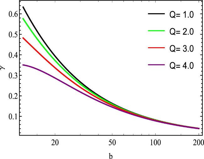
Figure 1. Coordination between γ and b for non-plasma field. |
In figure 2, we demonstrate the behavior of deflection angle γ regarding b for altering l and by taking the fixed value of M = 1, Q = 1, a = 0.3. We investigate that deflection angle geometrically increasing behavior for the increasing values l.
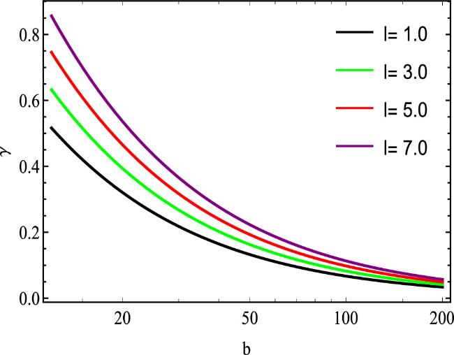
Figure 2. Coordination between γ and b for non-plasma field. |
In figure 3, we demonstrate the impact of the deflection angle γ in regards to b being fixed M = 1, Q = 1, l = 3 and varying a. We determined that the deflection angle constantly increases for letting greater values of a.

Figure 3. Coordination between γ and b for non-plasma field. |
4. Deflection angle around a gravitational decoupling extended black hole solution with graphical analysis for plasma case
In this section, we study weak gravitational lensing in the plasma medium due to the gravitational extended BH solution. The refractive index value u(r) [76] is expressed as14 and 18 .
$\begin{eqnarray}u(r)=\sqrt{1-\displaystyle \frac{{\omega }_{e}^{2}h(r)}{{\omega }_{\infty }^{2}}},\end{eqnarray}$
where ω∞ represents the photon frequency that is measured by an observer at and ωe represents the frequency of electron plasma. Assuming that both the source and the observers are situated on the equatorial plane, the null photon direction is on the same plane. The following is the associated metric function. $\begin{eqnarray}{{\rm{d}}{t}}^{2}={g}_{{ij}}^{{opt}}{{\rm{d}}{x}}^{i}{{\rm{d}}{x}}^{j}={u}^{2}(r)\left[\displaystyle \frac{{{\rm{d}}{r}}^{2}}{h{\left(r\right)}^{2}}+\displaystyle \frac{{r}^{2}{\rm{d}}{\phi }^{2}}{h(r)}\right].\end{eqnarray}$
The Christoffel symbols of non-zero values are shown as follows $\begin{eqnarray*}{{\rm{\Gamma }}}_{00}^{0}=\displaystyle \frac{-h{\left(r\right)}^{{\prime} }({\omega }_{e}^{2}h(r)-2{\omega }_{\infty }^{2})}{2h(r)({\omega }_{e}^{2}h(r)-{\omega }_{\infty }^{2})},\end{eqnarray*}$
$\begin{eqnarray*}{{\rm{\Gamma }}}_{11}^{0}=\displaystyle \frac{-r(h(r)^{\prime} r{\omega }_{\infty }^{2}+2h{\left(r\right)}^{2}{\omega }_{e}^{2}-2{\omega }_{\infty }^{2}h(r))}{{\omega }_{e}^{2}h(r)-{\omega }_{\infty }^{2}},\end{eqnarray*}$
$\begin{eqnarray*}{{\rm{\Gamma }}}_{01}^{1}={{\rm{\Gamma }}}_{10}^{1}=\displaystyle \frac{(h(r)^{\prime} r{\omega }_{\infty }^{2}+2h{\left(r\right)}^{2}{\omega }_{e}^{2}-2{\omega }_{\infty }^{2}h(r))}{2h(r)({\omega }_{e}^{2}h(r)-{\omega }_{\infty }^{2})}.\end{eqnarray*}$
It should be mentioned that to reduce complication, we use $N=\tfrac{{\omega }_{e}^{2}}{{\omega }_{\infty }^{2}}$ to calculate the deflection angle in the plasma medium. The non-zero Christoffel symbols can be used to compute the Gaussian curvature, as was previously described. $\begin{eqnarray*}\begin{array}{rcl}{ \mathcal K } & = & -\displaystyle \frac{66{a}^{2}{N}^{2}{M}^{4}}{{r}^{6}}-\displaystyle \frac{88{{aN}}^{2}{M}^{4}}{{r}^{6}}-\displaystyle \frac{44{N}^{2}{M}^{4}}{{r}^{6}}+\displaystyle \frac{12{{NM}}^{3}}{{r}^{5}}\\ & & +\displaystyle \frac{135{a}^{2}{N}^{2}{M}^{3}}{{r}^{5}}+\displaystyle \frac{150{{aN}}^{2}{M}^{3}}{{r}^{5}}+\displaystyle \frac{60{N}^{2}{M}^{3}}{{r}^{5}}-\displaystyle \frac{3{{aM}}^{2}}{{r}^{4}}\\ & & +\displaystyle \frac{9{a}^{2}{{NM}}^{3}}{{r}^{5}}+\displaystyle \frac{18{{aNM}}^{3}}{{r}^{5}}-\displaystyle \frac{132{a}^{2}{{lN}}^{2}{M}^{3}}{{r}^{6}}\\ & & -\displaystyle \frac{3{M}^{2}}{{r}^{4}}-\displaystyle \frac{88{{alN}}^{2}{M}^{3}}{{r}^{6}}+\displaystyle \frac{105{a}^{2}{N}^{2}{Q}^{2}{M}^{3}}{{r}^{7}}+\displaystyle \frac{210{{aN}}^{2}{Q}^{2}{M}^{3}}{{r}^{7}}\\ & & +\displaystyle \frac{140{N}^{2}{Q}^{2}{M}^{3}}{{r}^{7}}-\displaystyle \frac{81{{aN}}^{2}{M}^{2}}{{r}^{4}}-\displaystyle \frac{27{N}^{2}{M}^{2}}{{r}^{4}}-\displaystyle \frac{12{{NM}}^{2}}{{r}^{4}}\\ & & -\displaystyle \frac{15{a}^{2}{{NM}}^{2}}{{r}^{4}}-\displaystyle \frac{24{{aNM}}^{2}}{{r}^{4}}-\displaystyle \frac{3{a}^{2}{M}^{2}}{4{r}^{4}}-\displaystyle \frac{351{a}^{2}{N}^{2}{M}^{2}}{4{r}^{4}}\\ & & +\displaystyle \frac{180{a}^{2}{{lN}}^{2}{M}^{2}}{{r}^{5}}+\displaystyle \frac{90{{alN}}^{2}{M}^{2}}{{r}^{5}}-\displaystyle \frac{66{a}^{2}{l}^{2}{N}^{2}{M}^{2}}{{r}^{6}}+\displaystyle \frac{18{a}^{2}{{lNM}}^{2}}{{r}^{5}}\\ & & +\displaystyle \frac{18{{alNM}}^{2}}{{r}^{5}}+\displaystyle \frac{{a}^{2}M}{{r}^{3}}+\displaystyle \frac{18{a}^{2}{N}^{2}M}{{r}^{3}}\\ & & -\displaystyle \frac{324{{aN}}^{2}{Q}^{2}{M}^{2}}{{r}^{6}}-\displaystyle \frac{162{N}^{2}{Q}^{2}{M}^{2}}{{r}^{6}}-\displaystyle \frac{405{a}^{2}{N}^{2}{Q}^{2}{M}^{2}}{2{r}^{6}}-\displaystyle \frac{32{{aNQ}}^{2}{M}^{2}}{{r}^{6}}\\ & & -\displaystyle \frac{32{{NQ}}^{2}{M}^{2}}{{r}^{6}}-\displaystyle \frac{8{a}^{2}{{NQ}}^{2}{M}^{2}}{{r}^{6}}+\displaystyle \frac{3{aM}}{{r}^{3}}\\ & & +\displaystyle \frac{210{a}^{2}{{lN}}^{2}{Q}^{2}{M}^{2}}{{r}^{7}}+\displaystyle \frac{210{{alN}}^{2}{Q}^{2}{M}^{2}}{{r}^{7}}+\displaystyle \frac{14{{aN}}^{2}M}{{r}^{3}}+\displaystyle \frac{4{N}^{2}M}{{r}^{3}}\\ & & +\displaystyle \frac{6{a}^{2}{NM}}{{r}^{3}}+\displaystyle \frac{3{NM}}{{r}^{3}}-\displaystyle \frac{81{a}^{2}{l}^{2}{N}^{2}{Q}^{2}}{2{r}^{6}}-\displaystyle \frac{3{Q}^{2}}{{r}^{4}}\\ & & +\displaystyle \frac{2M}{{r}^{3}}+\displaystyle \frac{15{aNM}}{2{r}^{3}}-\displaystyle \frac{27{{alN}}^{2}M}{{r}^{4}}-\displaystyle \frac{3{alM}}{{r}^{4}}\\ & & -\displaystyle \frac{18{a}^{2}{lNM}}{{r}^{4}}-\displaystyle \frac{12{alNM}}{{r}^{4}}-\displaystyle \frac{135{a}^{2}{{lN}}^{2}M}{2{r}^{4}}-\displaystyle \frac{3{a}^{2}{lM}}{2{r}^{4}}+\displaystyle \frac{45{a}^{2}{l}^{2}{N}^{2}M}{{r}^{5}}\\ & & +\displaystyle \frac{120{a}^{2}{N}^{2}{Q}^{2}M}{{r}^{5}}+\displaystyle \frac{150{{aN}}^{2}{Q}^{2}M}{{r}^{5}}+\displaystyle \frac{60{N}^{2}{Q}^{2}M}{{r}^{5}}+\displaystyle \frac{3{{aQ}}^{2}M}{{r}^{5}}\\ & & +\displaystyle \frac{13{a}^{2}{{NQ}}^{2}M}{{r}^{5}}+\displaystyle \frac{39{{aNQ}}^{2}M}{{r}^{5}}+\displaystyle \frac{26{{NQ}}^{2}M}{{r}^{5}}\\ & & +\displaystyle \frac{6{Q}^{2}M}{{r}^{5}}+\displaystyle \frac{9{a}^{2}{l}^{2}{NM}}{{r}^{5}}-\displaystyle \frac{243{a}^{2}{{lN}}^{2}{Q}^{2}M}{{r}^{6}}+\displaystyle \frac{3{{alQ}}^{2}}{{r}^{5}}\\ & & -\displaystyle \frac{162{{alN}}^{2}{Q}^{2}M}{{r}^{6}}-\displaystyle \frac{16{a}^{2}{{lNQ}}^{2}M}{{r}^{6}}-\displaystyle \frac{32{{alNQ}}^{2}M}{{r}^{6}}+\displaystyle \frac{{al}}{{r}^{3}}\\ & & +\displaystyle \frac{105{a}^{2}{l}^{2}{N}^{2}{Q}^{2}M}{{r}^{7}}+\displaystyle \frac{6{a}^{2}{{lN}}^{2}}{{r}^{3}}+\displaystyle \frac{2{{alN}}^{2}}{{r}^{3}}+\displaystyle \frac{{a}^{2}l}{{r}^{3}}\\ & & -\displaystyle \frac{7{N}^{2}{Q}^{2}}{{r}^{4}}+\displaystyle \frac{3{a}^{2}{lN}}{{r}^{3}}+\displaystyle \frac{3{alN}}{2{r}^{3}}-\displaystyle \frac{21{a}^{2}{N}^{2}{Q}^{2}}{{r}^{4}}\end{array}\end{eqnarray*}$$\begin{eqnarray}\begin{array}{rcl} & & -\displaystyle \frac{21{{aN}}^{2}{Q}^{2}}{{r}^{4}}-\displaystyle \frac{5{{NQ}}^{2}}{{r}^{4}}-\displaystyle \frac{3{{aQ}}^{2}}{{r}^{4}}-\displaystyle \frac{5{a}^{2}{{NQ}}^{2}}{{r}^{4}}\\ & & -\displaystyle \frac{10{{aNQ}}^{2}}{{r}^{4}}-\displaystyle \frac{3{a}^{2}{l}^{2}}{4{r}^{4}}-\displaystyle \frac{27{a}^{2}{l}^{2}{N}^{2}}{4{r}^{4}}-\displaystyle \frac{3{a}^{2}{l}^{2}N}{{r}^{4}}\\ & & +\displaystyle \frac{60{a}^{2}{{lN}}^{2}{Q}^{2}}{{r}^{5}}+\displaystyle \frac{13{a}^{2}{{lNQ}}^{2}}{{r}^{5}}+\displaystyle \frac{13{{alNQ}}^{2}}{{r}^{5}}\\ & & +\displaystyle \frac{30{{alN}}^{2}{Q}^{2}}{{r}^{5}}-\displaystyle \frac{8{a}^{2}{l}^{2}{{NQ}}^{2}}{{r}^{6}}+O\left({Q}^{4},{N}^{3},{\alpha }^{3}\right).\end{array}\end{eqnarray}$
The value of the photon's deflection angle within the plasma framework is computed from equations $\begin{eqnarray}\begin{array}{rcl}\gamma & = & \displaystyle \frac{4M}{b}-\displaystyle \frac{3\pi {a}^{2}{l}^{2}}{16{b}^{2}}-\displaystyle \frac{3\pi {a}^{2}{lM}}{8{b}^{2}}-\displaystyle \frac{33{{aN}}^{2}\pi {M}^{4}}{4{b}^{4}}\\ & & +\displaystyle \frac{6{a}^{2}{lN}}{b}-\displaystyle \frac{33{N}^{2}\pi {M}^{4}}{8{b}^{4}}-\displaystyle \frac{99{a}^{2}{N}^{2}\pi {M}^{4}}{16{b}^{4}}+\displaystyle \frac{60{a}^{2}{N}^{2}{M}^{3}}{{b}^{3}}\\ & & -\displaystyle \frac{3\pi {Q}^{2}}{4{b}^{2}}+\displaystyle \frac{200{{aN}}^{2}{M}^{3}}{3{b}^{3}}+\displaystyle \frac{80{N}^{2}{M}^{3}}{3{b}^{3}}+\displaystyle \frac{112{a}^{2}{N}^{2}{Q}^{2}{M}^{3}}{5{b}^{5}}\\ & & +\displaystyle \frac{224{{aN}}^{2}{Q}^{2}{M}^{3}}{5{b}^{5}}+\displaystyle \frac{448{N}^{2}{Q}^{2}{M}^{3}}{15{b}^{5}}+\displaystyle \frac{4{a}^{2}{{NM}}^{3}}{{b}^{3}}\\ & & +\displaystyle \frac{8{{aNM}}^{3}}{{b}^{3}}+\displaystyle \frac{16{{NM}}^{3}}{3{b}^{3}}-\displaystyle \frac{33{{alN}}^{2}\pi {M}^{3}}{4{b}^{4}}\displaystyle \frac{3{a}^{2}{l}^{2}N\pi }{4{b}^{2}}\\ & & +\displaystyle \frac{80{a}^{2}{{lN}}^{2}{M}^{2}}{{b}^{3}}+\displaystyle \frac{40{{alN}}^{2}{M}^{2}}{{b}^{3}}+\displaystyle \frac{224{a}^{2}{{lN}}^{2}{Q}^{2}{M}^{2}}{5{b}^{5}}\\ & & +\displaystyle \frac{224{{alN}}^{2}{Q}^{2}{M}^{2}}{5{b}^{5}}+\displaystyle \frac{8{a}^{2}{{lNM}}^{2}}{{b}^{3}}+\displaystyle \frac{8{{alNM}}^{2}}{{b}^{3}}-\displaystyle \frac{6{aN}\pi {M}^{2}}{{b}^{2}}\\ & & -\displaystyle \frac{3N\pi {M}^{2}}{{b}^{2}}-\displaystyle \frac{81{{aN}}^{2}\pi {M}^{2}}{4{b}^{2}}-\displaystyle \frac{27{N}^{2}\pi {M}^{2}}{4{b}^{2}}-\displaystyle \frac{3a\pi {M}^{2}}{4{b}^{2}}\\ & & -\displaystyle \frac{15{a}^{2}N\pi {M}^{2}}{4{b}^{2}}-\displaystyle \frac{3\pi {M}^{2}}{4{b}^{2}}-\displaystyle \frac{3{a}^{2}\pi {M}^{2}}{16{b}^{2}}-\displaystyle \frac{351{a}^{2}{N}^{2}\pi {M}^{2}}{16{b}^{2}}\\ & & -\displaystyle \frac{3{aN}\pi {Q}^{2}{M}^{2}}{{b}^{4}}-\displaystyle \frac{3N\pi {Q}^{2}{M}^{2}}{{b}^{4}}-\displaystyle \frac{3{a}^{2}N\pi {Q}^{2}{M}^{2}}{4{b}^{4}}+\displaystyle \frac{8{N}^{2}M}{b}\\ & & -\displaystyle \frac{243{{aN}}^{2}\pi {Q}^{2}{M}^{2}}{8{b}^{4}}-\displaystyle \frac{243{N}^{2}\pi {Q}^{2}{M}^{2}}{16{b}^{4}}-\displaystyle \frac{99{a}^{2}{l}^{2}{N}^{2}\pi {M}^{2}}{16{b}^{4}}-\displaystyle \frac{1215{a}^{2}{N}^{2}\pi {Q}^{2}{M}^{2}}{64{b}^{4}}\\ & & +\displaystyle \frac{20{a}^{2}{l}^{2}{N}^{2}M}{{b}^{3}}+\displaystyle \frac{36{a}^{2}{N}^{2}M}{b}\\ & & +\displaystyle \frac{28{{aN}}^{2}M}{b}+\displaystyle \frac{112{a}^{2}{l}^{2}{N}^{2}{Q}^{2}M}{5{b}^{5}}+\displaystyle \frac{160{a}^{2}{N}^{2}{Q}^{2}M}{3{b}^{3}}+\displaystyle \frac{200{{aN}}^{2}{Q}^{2}M}{3{b}^{3}}\\ & & +\displaystyle \frac{80{N}^{2}{Q}^{2}M}{3{b}^{3}}+\displaystyle \frac{52{{aNQ}}^{2}M}{3{b}^{3}}+\displaystyle \frac{12{a}^{2}{NM}}{b}\\ & & +\displaystyle \frac{104{{NQ}}^{2}M}{9{b}^{3}}+\displaystyle \frac{4{{aQ}}^{2}M}{3{b}^{3}}+\displaystyle \frac{8{Q}^{2}M}{3{b}^{3}}+\displaystyle \frac{4{a}^{2}{l}^{2}{NM}}{{b}^{3}}+\displaystyle \frac{15{aNM}}{b}\\ & & +\displaystyle \frac{6{NM}}{b}+\displaystyle \frac{2{a}^{2}M}{b}+\displaystyle \frac{6{aM}}{b}-\displaystyle \frac{3{alN}\pi M}{{b}^{2}}\\ & & -\displaystyle \frac{27{{alN}}^{2}\pi M}{4{b}^{2}}-\displaystyle \frac{3{al}\pi M}{4{b}^{2}}-\displaystyle \frac{135{a}^{2}{{lN}}^{2}\pi M}{8{b}^{2}}-\displaystyle \frac{3{alN}\pi {Q}^{2}M}{{b}^{4}}\\ & & -\displaystyle \frac{3{a}^{2}{lN}\pi {Q}^{2}M}{2{b}^{4}}-\displaystyle \frac{243{{alN}}^{2}\pi {Q}^{2}M}{16{b}^{4}}-\displaystyle \frac{729{a}^{2}{{lN}}^{2}\pi {Q}^{2}M}{32{b}^{4}}\\ & & +\displaystyle \frac{12{a}^{2}{{lN}}^{2}}{b}+\displaystyle \frac{4{{alN}}^{2}}{b}+\displaystyle \frac{80{a}^{2}{{lN}}^{2}{Q}^{2}}{3{b}^{3}}+\displaystyle \frac{40{{alN}}^{2}{Q}^{2}}{3{b}^{3}}\\ & & +\displaystyle \frac{4{{alQ}}^{2}}{3{b}^{3}}+\displaystyle \frac{52{a}^{2}{{lNQ}}^{2}}{9{b}^{3}}+\displaystyle \frac{52{{alNQ}}^{2}}{9{b}^{3}}+\displaystyle \frac{2{a}^{2}l}{b}+\displaystyle \frac{2{al}}{b}\\ & & +\displaystyle \frac{3{alN}}{b}-\displaystyle \frac{5{aN}\pi {Q}^{2}}{2{b}^{2}}-\displaystyle \frac{21{a}^{2}{N}^{2}\pi {Q}^{2}}{4{b}^{2}}-\displaystyle \frac{21{{aN}}^{2}\pi {Q}^{2}}{4{b}^{2}}\\ & & -\displaystyle \frac{7{N}^{2}\pi {Q}^{2}}{4{b}^{2}}-\displaystyle \frac{3a\pi {Q}^{2}}{4{b}^{2}}-\displaystyle \frac{5{a}^{2}N\pi {Q}^{2}}{4{b}^{2}}-\displaystyle \frac{5N\pi {Q}^{2}}{4{b}^{2}}\\ & & -\displaystyle \frac{27{a}^{2}{l}^{2}{N}^{2}\pi }{16{b}^{2}}-\displaystyle \frac{3{a}^{2}{l}^{2}N\pi {Q}^{2}}{4{b}^{4}}-\displaystyle \frac{243{a}^{2}{l}^{2}{N}^{2}\pi {Q}^{2}}{64{b}^{4}}+\displaystyle \frac{52{a}^{2}{{NQ}}^{2}M}{9{b}^{3}}\\ & & -\displaystyle \frac{9{a}^{2}{lN}\pi M}{2{b}^{2}}-\displaystyle \frac{99{a}^{2}{{lN}}^{2}\pi {M}^{3}}{8{b}^{4}}.\end{array}\end{eqnarray}$
In the framework of the plasma medium, now we will examine the graphical effects of the deflection angle. By examining these graphs, we see how the plasma surroundings behave.
In figure 4, we demonstrate the behaviour of the deflection angle γ along b for constant values of M = 1, N = 0.05, l = 3, a = 0.3 and for the different values of Q. We viewed that the deflection angle gradually shows the increasing behaviour for decreasing values of Q.

Figure 4. Coordination between γ and b for plasma field. |
In figure 5, we present the influence of the deflection angle γ along b for constant values of M = 1, N = 0.05, Q = 1, a = 0.3 and by changing l. We notice the deflection angle steadily increasing for increasing value of l.
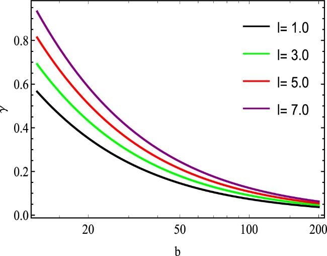
Figure 5. Coordination between γ and b for plasma field. |
In figure 6, we demonstrate the influence of the deflection angle γ with comparison to impact parameter b for fixed values of M = 1, N = 0.05, Q = 1, l = 3 and by altering a. We observed that the deflection angle gradually increased for the larger value of a and gradually decreased for smaller values.
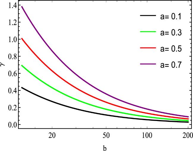
Figure 6. Coordination between γ and b for plasma field. |
In figure 7, we analyzed the conduct of deflection angle γ versus b for the different values of N and fixed values of of M = 1, a = 0.3, Q = 1, l = 3. We see that for the smaller values of N deflection angle is gradually small but for the larger value of N deflection angle shows the increasing behaviour.
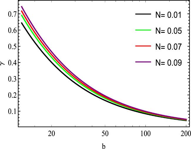
Figure 7. Coordination between γ and b for plasma field. |
The weak-field limit in the context of a BH is associated with distances that are far from the event horizon when the gravitational field is weak. In this instance, there is very little influence on the deflection angle from hairy parameters such as (Q, l, and a). This is because other elements, such as hairy parameters, are small perturbations that may be ignored, and the object's mass dominates the gravitational field. Conversely, distances near the event horizon correspond to the strong-field limit. Since the strong-field effect on hairy parameters is more substantial, the gravitational field is significantly stronger and has a greater impact on the parameters. We have magnified the graphs for the wake deflection results. For both the plasma and non-plasma scenarios, we can observe that the trajectories are nearly identical because of the wake gravitational field. However, the deflection angle curves are more spaced apart in a strong gravitational field case.
5. Lens equation and Einstein ring in gravitational lensing by black hole
Light beams from distant brilliant light sources can be deflected or distorted by a galaxy's central supermassive BH. Eventually, many images might be displayed as a result of these intense light sources light beams. The gravitational lens equation is the main constraint on the Einstein ring and other important physical observable in gravitational lensing observations. One can use lenses and the Einstein ring to calculate the locations of objects using the lens equation. In the previous few decades, many gravitational lens equations have been devised [51, 77–83]. We utilize a well-known lens equation given by Bozza [78] in this work.21 ) indicates the visible angular position of the lensed picture as viewed by a distant observer, while angle β indicates the precise angular position of the strong light source. Eventually, this lens equation can be used to retrieve the images of the lensed objects. The approximations tan β ≈ β, $\sin \theta \approx \theta $, and $\sin (\gamma -\theta )\approx \gamma -\theta $ for distant sources and observers are available in the strong deflection limit. By decreasing the lens equation (21 ) [84], the following form is obtained.
$\begin{eqnarray}{D}_{\mathrm{OS}}\tan \beta =\displaystyle \frac{{D}_{\mathrm{OS}}\sin \theta -{D}_{\mathrm{LS}}\sin (\gamma -\theta )}{\cos (\gamma -\theta )}.\end{eqnarray}$
The distances in this instance between the lens plane and source plane (DOS), the source plane and the observer (DLS), and the source plane and the source plane are shown by, DOS, and DLS. Angle θ in equation ( $\begin{eqnarray}\beta =\theta -\displaystyle \frac{{D}_{\mathrm{LS}}}{{D}_{\mathrm{OS}}}\gamma .\end{eqnarray}$
The formula DOS = DOL + DLS was used to derive the equation. The angular radius of the Einstein ring can be found by using β = 0. $\begin{eqnarray}{\theta }_{E}=\displaystyle \frac{{D}_{\mathrm{LS}}}{{D}_{\mathrm{OS}}}\gamma .\end{eqnarray}$
The modified gravitational lens equation and the weak deflection limit are the main topics of discussion in this section. The Einstein ring angle θE for the gravitational decoupling extended BH solution can be derived as for the non-plasma: $\begin{eqnarray}\begin{array}{rcl}{\theta }_{E} & = & \displaystyle \frac{{D}_{\mathrm{LS}}}{{D}_{\mathrm{OS}}}\left(\displaystyle \frac{4M}{b}-\displaystyle \frac{3\pi {a}^{2}{l}^{2}}{16{b}^{2}}-\displaystyle \frac{3\pi {a}^{2}{lM}}{8{b}^{2}}-\displaystyle \frac{3\pi {a}^{2}{M}^{2}}{16{b}^{2}}\right.\\ & & +\displaystyle \frac{2{a}^{2}l}{b}+\displaystyle \frac{2{a}^{2}M}{b}+\displaystyle \frac{4{{alQ}}^{2}}{3{b}^{3}}+\displaystyle \frac{4{{aMQ}}^{2}}{3{b}^{3}}-\displaystyle \frac{3\pi {alM}}{4{b}^{2}}\\ & & -\displaystyle \frac{3\pi {{aM}}^{2}}{4{b}^{2}}-\displaystyle \frac{3\pi {{aQ}}^{2}}{4{b}^{2}}+\displaystyle \frac{2{al}}{b}++\displaystyle \frac{6{aM}}{b}\\ & & \left.+\displaystyle \frac{8{{MQ}}^{2}}{3{b}^{3}}-\displaystyle \frac{3\pi {M}^{2}}{4{b}^{2}}-\displaystyle \frac{3\pi {Q}^{2}}{4{b}^{2}}\right),\end{array}\end{eqnarray}$
and plasma scenario: $\begin{eqnarray*}\begin{array}{rcl}{\theta }_{E} & = & \displaystyle \frac{{D}_{\mathrm{LS}}}{{D}_{\mathrm{OS}}}\left(\displaystyle \frac{4M}{b}-\displaystyle \frac{3\pi {a}^{2}{l}^{2}}{16{b}^{2}}-\displaystyle \frac{3\pi {a}^{2}{lM}}{8{b}^{2}}\right.\\ & & -\displaystyle \frac{33{{aN}}^{2}\pi {M}^{4}}{4{b}^{4}}-\displaystyle \frac{33{N}^{2}\pi {M}^{4}}{8{b}^{4}}-\displaystyle \frac{99{a}^{2}{N}^{2}\pi {M}^{4}}{16{b}^{4}}+\displaystyle \frac{60{a}^{2}{N}^{2}{M}^{3}}{{b}^{3}}\\ & & -\,\displaystyle \frac{3\pi {Q}^{2}}{4{b}^{2}}+\displaystyle \frac{200{{aN}}^{2}{M}^{3}}{3{b}^{3}}+\displaystyle \frac{80{N}^{2}{M}^{3}}{3{b}^{3}}+\displaystyle \frac{112{a}^{2}{N}^{2}{Q}^{2}{M}^{3}}{5{b}^{5}}\\ & & +\,\displaystyle \frac{224{{aN}}^{2}{Q}^{2}{M}^{3}}{5{b}^{5}}+\displaystyle \frac{448{N}^{2}{Q}^{2}{M}^{3}}{15{b}^{5}}+\displaystyle \frac{4{a}^{2}{{NM}}^{3}}{{b}^{3}}\\ & & +\displaystyle \frac{8{{aNM}}^{3}}{{b}^{3}}+\displaystyle \frac{16{{NM}}^{3}}{3{b}^{3}}-\displaystyle \frac{33{{alN}}^{2}\pi {M}^{3}}{4{b}^{4}}\displaystyle \frac{3{a}^{2}{l}^{2}N\pi }{4{b}^{2}}+\displaystyle \frac{80{a}^{2}{{lN}}^{2}{M}^{2}}{{b}^{3}}\\ & & +\displaystyle \frac{40{{alN}}^{2}{M}^{2}}{{b}^{3}}+\displaystyle \frac{224{a}^{2}{{lN}}^{2}{Q}^{2}{M}^{2}}{5{b}^{5}}\\ & & +\displaystyle \frac{224{{alN}}^{2}{Q}^{2}{M}^{2}}{5{b}^{5}}+\displaystyle \frac{8{a}^{2}{{lNM}}^{2}}{{b}^{3}}+\displaystyle \frac{8{{alNM}}^{2}}{{b}^{3}}-\displaystyle \frac{6{aN}\pi {M}^{2}}{{b}^{2}}\\ & & -\displaystyle \frac{3N\pi {M}^{2}}{{b}^{2}}-\displaystyle \frac{81{{aN}}^{2}\pi {M}^{2}}{4{b}^{2}}-\displaystyle \frac{27{N}^{2}\pi {M}^{2}}{4{b}^{2}}-\displaystyle \frac{3a\pi {M}^{2}}{4{b}^{2}}\\ & & -\displaystyle \frac{15{a}^{2}N\pi {M}^{2}}{4{b}^{2}}-\displaystyle \frac{3\pi {M}^{2}}{4{b}^{2}}-\displaystyle \frac{3{a}^{2}\pi {M}^{2}}{16{b}^{2}}-\displaystyle \frac{351{a}^{2}{N}^{2}\pi {M}^{2}}{16{b}^{2}}\\ & & -\displaystyle \frac{3{aN}\pi {Q}^{2}{M}^{2}}{{b}^{4}}-\displaystyle \frac{3N\pi {Q}^{2}{M}^{2}}{{b}^{4}}-\displaystyle \frac{3{a}^{2}N\pi {Q}^{2}{M}^{2}}{4{b}^{4}}+\displaystyle \frac{8{N}^{2}M}{b}\\ & & -\displaystyle \frac{243{{aN}}^{2}\pi {Q}^{2}{M}^{2}}{8{b}^{4}}-\displaystyle \frac{243{N}^{2}\pi {Q}^{2}{M}^{2}}{16{b}^{4}}-\displaystyle \frac{99{a}^{2}{l}^{2}{N}^{2}\pi {M}^{2}}{16{b}^{4}}\\ & & -\,\displaystyle \frac{1215{a}^{2}{N}^{2}\pi {Q}^{2}{M}^{2}}{64{b}^{4}}+\displaystyle \frac{20{a}^{2}{l}^{2}{N}^{2}M}{{b}^{3}}+\displaystyle \frac{36{a}^{2}{N}^{2}M}{b}\\ & & +\displaystyle \frac{28{{aN}}^{2}M}{b}+\displaystyle \frac{112{a}^{2}{l}^{2}{N}^{2}{Q}^{2}M}{5{b}^{5}}+\displaystyle \frac{160{a}^{2}{N}^{2}{Q}^{2}M}{3{b}^{3}}\\ & & +\,\displaystyle \frac{200{{aN}}^{2}{Q}^{2}M}{3{b}^{3}}+\displaystyle \frac{80{N}^{2}{Q}^{2}M}{3{b}^{3}}+\displaystyle \frac{52{{aNQ}}^{2}M}{3{b}^{3}}+\displaystyle \frac{12{a}^{2}{NM}}{b}\\ & & +\displaystyle \frac{104{{NQ}}^{2}M}{9{b}^{3}}+\displaystyle \frac{4{{aQ}}^{2}M}{3{b}^{3}}+\displaystyle \frac{8{Q}^{2}M}{3{b}^{3}}+\displaystyle \frac{4{a}^{2}{l}^{2}{NM}}{{b}^{3}}\\ & & +\displaystyle \frac{15{aNM}}{b}+\displaystyle \frac{6{NM}}{b}+\displaystyle \frac{2{a}^{2}M}{b}+\displaystyle \frac{6{aM}}{b}-\displaystyle \frac{3{alN}\pi M}{{b}^{2}}\end{array}\end{eqnarray*}$$\begin{eqnarray*}\begin{array}{rcl} & & -\displaystyle \frac{27{{alN}}^{2}\pi M}{4{b}^{2}}-\displaystyle \frac{3{al}\pi M}{4{b}^{2}}-\displaystyle \frac{135{a}^{2}{{lN}}^{2}\pi M}{8{b}^{2}}-\displaystyle \frac{3{alN}\pi {Q}^{2}M}{{b}^{4}}\\ & & -\displaystyle \frac{3{a}^{2}{lN}\pi {Q}^{2}M}{2{b}^{4}}-\displaystyle \frac{243{{alN}}^{2}\pi {Q}^{2}M}{16{b}^{4}}-\displaystyle \frac{729{a}^{2}{{lN}}^{2}\pi {Q}^{2}M}{32{b}^{4}}\\ & & +\displaystyle \frac{12{a}^{2}{{lN}}^{2}}{b}+\displaystyle \frac{4{{alN}}^{2}}{b}+\displaystyle \frac{80{a}^{2}{{lN}}^{2}{Q}^{2}}{3{b}^{3}}+\displaystyle \frac{40{{alN}}^{2}{Q}^{2}}{3{b}^{3}}\\ & & +\displaystyle \frac{4{{alQ}}^{2}}{3{b}^{3}}+\displaystyle \frac{52{a}^{2}{{lNQ}}^{2}}{9{b}^{3}}+\displaystyle \frac{52{{alNQ}}^{2}}{9{b}^{3}}+\displaystyle \frac{2{a}^{2}l}{b}+\displaystyle \frac{2{al}}{b}\\ & & +\displaystyle \frac{3{alN}}{b}-\displaystyle \frac{5{aN}\pi {Q}^{2}}{2{b}^{2}}-\displaystyle \frac{21{a}^{2}{N}^{2}\pi {Q}^{2}}{4{b}^{2}}-\displaystyle \frac{21{{aN}}^{2}\pi {Q}^{2}}{4{b}^{2}}\\ & & -\displaystyle \frac{7{N}^{2}\pi {Q}^{2}}{4{b}^{2}}-\displaystyle \frac{3a\pi {Q}^{2}}{4{b}^{2}}-\displaystyle \frac{5{a}^{2}N\pi {Q}^{2}}{4{b}^{2}}-\displaystyle \frac{5N\pi {Q}^{2}}{4{b}^{2}}\\ & & -\displaystyle \frac{27{a}^{2}{l}^{2}{N}^{2}\pi }{16{b}^{2}}-\displaystyle \frac{3{a}^{2}{l}^{2}N\pi {Q}^{2}}{4{b}^{4}}-\displaystyle \frac{243{a}^{2}{l}^{2}{N}^{2}\pi {Q}^{2}}{64{b}^{4}}\end{array}\end{eqnarray*}$$\begin{eqnarray}\begin{array}{l}\,+\,\displaystyle \frac{52{a}^{2}{{NQ}}^{2}M}{9{b}^{3}}-\displaystyle \frac{9{a}^{2}{lN}\pi M}{2{b}^{2}}-\displaystyle \frac{99{a}^{2}{{lN}}^{2}\pi {M}^{3}}{8{b}^{4}}\left.+\displaystyle \frac{6{a}^{2}{lN}}{b}\right).\end{array}\end{eqnarray}$
In figures 8, 9 and 10, we plot the Einstein ring angle along the line $\tfrac{{D}_{\mathrm{LS}}}{{D}_{\mathrm{OS}}}$. We set the parameter Q, l, a to a distinct value for each graph respectively, and we fix M = b = 1, N = 0.005. The Einstein ring angle is plotted for each of the several $\tfrac{{D}_{\mathrm{LS}}}{{D}_{\mathrm{OS}}}$ ratios. The Einstein ring gets bigger when $\tfrac{{D}_{\mathrm{LS}}}{{D}_{\mathrm{OS}}}$ is larger. Amazing images of Einstein rings can only be observed at the largest distance DLS. We also noticed that the pattern of the Einstein ring angle is similar for both plasma and non-plasma fields.
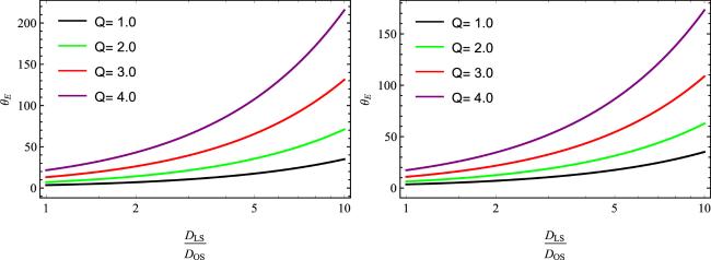
Figure 8. The Einstein ring angle θE versus ratio $\tfrac{{D}_{\mathrm{LS}}}{{D}_{\mathrm{OS}}}$ for non-plasma (left plot) and plasma case (right plot). |
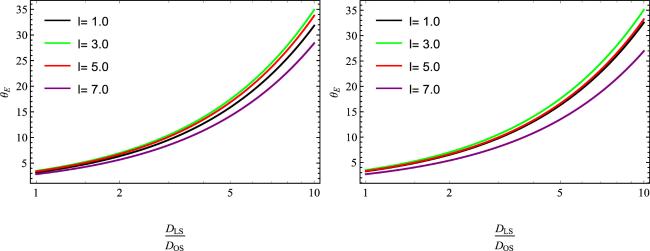
Figure 9. The Einstein ring angle θE versus ratio $\tfrac{{D}_{\mathrm{LS}}}{{D}_{\mathrm{OS}}}$ for non-plasma (left plot) and plasma case (right plot). |
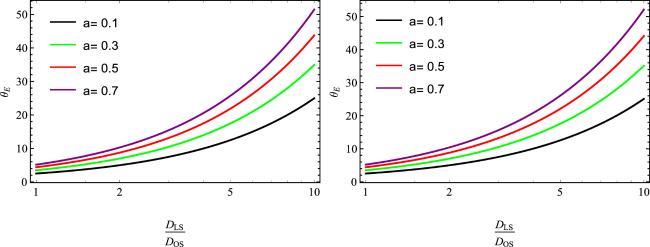
Figure 10. The Einstein ring angle θE versus ratio $\tfrac{{D}_{\mathrm{LS}}}{{D}_{\mathrm{OS}}}$ for non-plasma (left plot) and plasma case (right plot). |
6. Oscillations of massive particles near the circular orbit
This section is devoted to investigating the epicyclic frequencies related to the QPOs of test particles in the effective region of the radius of the innermost stable circular orbit (ISCO). You may obtain a more thorough formulation of these frequencies from [85]. We take into consideration three different sorts of fundamental frequencies: (i) the Keplerian frequency, also known as the orbital frequency ${v}_{\phi }=\tfrac{{w}_{\phi }}{2\pi }$. (ii) The radial epicyclic frequency is ${v}_{r}=\tfrac{{w}_{r}}{2\pi }$, and (iii) the vertical epicyclic frequency is ${v}_{\theta }=\tfrac{{w}_{\theta }}{2\pi }$ which is the frequency of the vertical oscillations around the mean orbit, describing the temporal behavior of time like equatorial circular orbits. We possess:5 ).
$\begin{eqnarray}{w}_{\phi }=\displaystyle \frac{{\rm{d}}\phi }{{\rm{d}}t}=\displaystyle \frac{-\tfrac{\partial {g}_{t\phi }}{\partial r}\pm \sqrt{{\left(\tfrac{\partial {g}_{t\phi }}{\partial r}\right)}^{2}-\tfrac{\partial {g}_{H}}{\partial r}\tfrac{\partial {g}_{\phi \phi }}{\partial r}}}{\tfrac{\partial {g}_{\phi \phi }}{\partial r}},\end{eqnarray}$
$\begin{eqnarray}{w}_{r}^{2}=-\displaystyle \frac{1}{2{i}^{2}{g}_{{rr}}}\displaystyle \frac{{\partial }^{2}{V}_{\mathrm{eff}}}{\partial {r}^{2}},\end{eqnarray}$
$\begin{eqnarray}{w}_{\theta }^{2}=-\displaystyle \frac{1}{2{t}^{2}{g}_{\theta \theta }}\displaystyle \frac{{\partial }^{2}{V}_{\mathrm{eff}}}{\partial {\theta }^{2}}.\end{eqnarray}$
The fundamental frequencies of huge particles that move around the circular orbits can be found in the following form in the metric space provided by equation ( $\begin{eqnarray*}\begin{array}{rcl}{v}_{r} & = & \displaystyle \frac{\sqrt{{v}_{1r}}}{2\sqrt{2}\pi },\ \Rightarrow \\ {v}_{1r} & = & \displaystyle \frac{\left(r(a(l+M-r)+2M-r)-{Q}^{2}\right)}{{r}^{6}{\left(r(-3a(l+M)+2{ar}-6M+2r)+4{Q}^{2}\right)}^{3}}\left[-4r\left(r(a(l+M)+2M)-2{Q}^{2}\right)\right.\\ & & \times \,\left[r\left[a(-3l-3M+2r)-6M+2r\right]+4{Q}^{2}\right]\left({a}^{2}{r}^{2}(l+M)+a\left(l\left({Q}^{2}+{r}^{2}\right)+{{MQ}}^{2}+3{{Mr}}^{2}-4{Q}^{2}r\right)\right.\\ & & \left.+\,2\left(M\left({Q}^{2}+{r}^{2}\right)-2{Q}^{2}r\right)\right)\\ & & +\,{r}^{2}\left(-\left(r(-a(l+M-r)-2M+r)+{Q}^{2}\right)\right)\\ & & \times \,\left[-2{\left(a(3l+3M-4r)+6M-4r\right)}^{2}\left[r(a(l+M)+2M)-2{Q}^{2}\right]\right.\\ & & +\,2(a(l+M)+2M)(a(3l+3M-4r)+6M-4r)\left(r(a(3l+3M-2r)+6M-2r)-4{Q}^{2}\right)\\ & & -\,4(a+1)(2{Q}^{2}-r(a(l+M)+2M))(r(-3a(l+M)+2{ar}-6M+2r)+4{Q}^{2})]\\ & & \left.\left.+\,4[3{Q}^{2}-r[a(l+M)+2M\right]\right]\\ & & \times \,\left(r(-a(l+M-r)-2M+r)+{Q}^{2}\right)\\ & & \left.\times \,{\left(r(a(-3l-3M+2r)-6M+2r)+4{Q}^{2}\right)}^{2}\right].\\ {v}_{\phi }={v}_{\theta } & = & \displaystyle \frac{\sqrt{r(a(l+M)+2M)-2{Q}^{2}}}{2\sqrt{2}\pi {r}^{2}}.\end{array}\end{eqnarray*}$
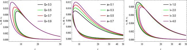
The spacetime parameters a, Q, l determine the behavior of these frequencies, which we plot in figure 11. From this figure 11, one can observe both overall increasing and decreasing values of these frequencies, and more specifically, that the values of vr, vθ vary with the variation in a, Q, l.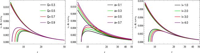
Figure 11. Upper and lower frequencies: the left plot shows variations of Q, the middle plot shows variations of a, and the right plot shows variations of l. |
We consider the potential frequency of twin peak QPOs [86] around the gravitational decoupling extended black hole in this section of the manuscript.
According to the conventional relativistic procession (RP) model [87], the higher and lower frequencies are vU = vφ and vL = vφ − vr, respectively, based on the radial and tangential frequencies. While the frequencies in the modified RP2 model are given as vU = vφ, vL = vθ − vr, the frequencies in the modified RP1 model are represented as vU = vθ, vL = vφ − vr. Figure 12 presents a graphical study of the RP model (with increasing and decreasing behaviors) by varying model parameters.
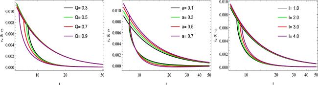
Figure 12. RP1 model: the left plot shows variations of Q, the middle plot shows variations of a, and the right plot shows variations of l. |
According to [88], the three models describing epicyclic resonances are represented by the letters ER2, ER3, and ER4. It is hypothesized that in these models, the accretion discs are significantly thick, and QPOs arise from the resonance of regular radiation particles along geodesic orbits. For the ER models, the following are the upper and lower frequencies of the orbital and epicyclic oscillations: vU = 2vθ − vr and vL=vr are the ER2 model equations. vU = vθ + vr and vL = vθ are the equations for the ER3 model. Lastly, vU = vθ + vr and vL = vθ − vr are the formulas for the ER4 model. Figures 13 14, 15 show plots of the ER models (ER2, ER3, ER4) with parameters a, Q, and l, encompassing all gravitational decoupling effects in an extended BH geometry.
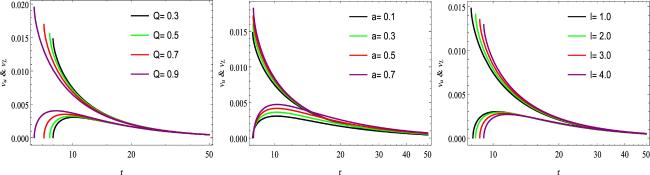
Figure 13. ER2 model: the left plot shows variations of Q, the middle plot shows variations of a, and the right plot shows variations of l. |
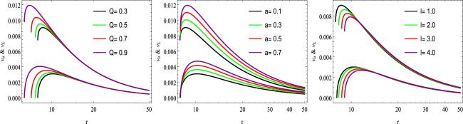
Figure 14. ER3 model: the left plot shows variations of Q, the middle plot shows variations of a, and the right plot shows variations of l. |
Figure 15. ER4 model: the left plot shows variations of Q, the middle plot shows variations of a, and the right plot shows variations of l. |
7. Summary
In this paper, we present the deflection angle for the gravitational decoupling extended BH solution. In our recent investigation, we studied the deflection angle for non-plasma and plasma fields. We consider the most valuable tool designed by Gibbon and Werner. We use the Gauss–Bonnet theorem to determine the result for the photon's deflection angle which includes a domain region outside of b (impact parameter). This represents the global effect of gravitational lensing and has a powerful apparatus that probes the prime of the BH singularities. Due to our analysis, we can calculate the photon deflection angle for the gravitational decoupling BH solution in weak-field limits using the method of GBT. For the non-plasma case, our proposed deflection angle in equation (16 ) is reduced into the Schwarzschild BH deflection angle up to the leading terms by letting α = 0, Q = 0, [89].
$\begin{eqnarray*}\gamma =\displaystyle \frac{4M}{b}.\end{eqnarray*}$
Similarly, we calculated the photon deflection angle for gravitational decoupling extended BH solution when plasma medium is available. In equation (20) , our computed deflection angle also reduced up to the leading terms of the well-known Schwarzschild BH deflection angle by putting α = 0, Q = 0.
To remove the plasma effect $\tfrac{{\omega }_{e}^{2}}{{\omega }_{\infty }^{2}}=N$, the deflection angle for plasma equation (20 ) is converted into equation (16 ) for the leading order. Furthermore, we discuss the deflection angle graphically for the various values of deflection angle to the background of plasma and non-plasma medium. We notice graphically that, the calculated deflection angle exhibits a similar pattern for both cases. Additionally, we determine the Einstein ring's size. The distance DLS should be as large as possible for exceptional Einstein ring images.
We also discuss the QPOs by discussing the radial and tangential frequencies and based on these radial and tangential frequencies, we further discuss the upper and lower frequencies categorized by the RP1 model, and the ER2, ER3, ER4 models. We noticed that model parameters a, l, Q have a significant impact on the behavior of these frequencies in increasing and decreasing terms.