


1. Introduction
The task of solving nonlinear partial differential equations (PDEs) is crucial across a spectrum of scientific and engineering fields. [1–5] Diverse methodologies have been employed to investigate soliton solutions of PDEs, including the inverse scatter method [6], the exp-function method [7, 8], Darboux transformation [9, 10], the multi-variable separation method [11], spontaneous symmetry method [12], the Hirota bilinear method [13], and so on [14, 15]. Among the methods listed above, the Hirota bilinear method [13] stands out as it involves transforming the model into a bilinear form using Hirota’s derivative operator, coupled with an appropriate variable change. This approach is commonly employed to derive solutions for integrable nonlinear equations, including N-soliton solutions [16], lump solutions [17, 18], breathers [18, 19], rogue waves [20–22] and their interaction solutions [23–25].
The advent of neural networks has engendered a novel approach that integrates the bilinear method with neural network architectures, termed the bilinear neural network method (BNNM) [26–30]. Diverging from methods like physics-informed neural networks (PINNs) [31–34], which construct loss functions through boundary or initial conditions, the BNNM obtains solutions by flexibly constructing a variety of exact analytical activation functions. Recent advancements, including the bilinear residual network method [35, 36] and the multivariate BNNM [37], have significantly enhanced the BNNM’s ability to solve complex differential equations.
The primary objective of this paper is to employ this method in computing the following (2+1)-dimensional nonlinear evolution equation [38]:2 ) is studied by Hua et al [38] and the rational wave solutions are retrieved through adopting the simplied Hirota’s method as well as ansatz approaches by Hosseini et al [39].
$\begin{eqnarray}\begin{array}{l}{u}_{{yt}}+{c}_{1}\left[{u}_{{xxxy}}+3(2{u}_{x}{u}_{y}+{u}_{{xy}}u)+3{u}_{{xx}}\displaystyle \int {u}_{y}{\rm{d}}x\right]\\ \,+\,{c}_{2}{u}_{{yy}}=0,\end{array}\end{eqnarray}$
where c1 and c2 are arbitrary constants. This equation represents a generalized model designed to explain the nonlinear dynamical phenomena occurring in shallow water environments. It can be reformulated as a generalized (2+1)-dimensional Hirota bilinear equation expressed as $\begin{eqnarray}\begin{array}{l}({{\rm{D}}}_{t}{{\rm{D}}}_{y}+{c}_{1}{{\rm{D}}}_{x}^{3}{{\rm{D}}}_{y}+{c}_{2}{{\rm{D}}}_{y}^{2})f\cdot f\\ \,=\,2[{f}_{{yt}}f-{f}_{y}{f}_{t}+{c}_{1}({f}_{{xxxy}}f-3{f}_{{xxy}}{f}_{x}+3{f}_{{xy}}{f}_{{xx}}-{f}_{y}{f}_{{xxx}})\\ \,+\,{c}_{2}({f}_{{yy}}f-{f}_{y}^{2})]=0,\end{array}\end{eqnarray}$
under the dependent variable transformation $\begin{eqnarray}u=2{\left(\mathrm{ln}f\right)}_{{xx}}.\end{eqnarray}$
The interaction behavior of equation (Currently, the BNNM has not yet been applied to solve this equation. This paper introduces the BNNM to study the (2+1)-dimensional Hirota bilinear equation. Following sections of the paper will outline the principles and implementation of the BNNM in section 2 . In sections 3 and 4 , various solutions to this equation will be presented by utilizing a single-layer model and a double-layer model, respectively. Section 5 will provide conclusions and outlooks.
2. Bilinear neural network method
In this section, a method called BNNM will be introduced, which utilizes a neural network model comprising n hidden layers to solve the exact analytical solution of the system. The tensor formula of the BNNM is constructed in the following form:
$\begin{eqnarray}f={\omega }_{{l}_{n},f}{F}_{{l}_{n}}({\xi }_{{l}_{n}}),\end{eqnarray}$
where ωa,b is the weight coefficient of neuron a to b and F is a generalized activation function, which can be defined arbitrarily but must be satisfied ${F}_{{l}_{n}}\geqslant 0$ in the last hidden layer. ${\xi }_{{l}_{i}}$ is given as follows: $\begin{eqnarray}{\xi }_{{l}_{i}}={\omega }_{{l}_{i-1},{l}_{i}}{F}_{{l}_{i-1}}({\xi }_{{l}_{i-1}})+{b}_{{l}_{i}},\quad i=1,2,\ldots ,\,n,\end{eqnarray}$
where l0 = {x, y, ⋯ , t}, li = {σi,1, σi,2, ⋯ , σi,m}, m denotes the number of neurons in the layer and b represents the bias of the layers, easily understood as a constant here. The equation represents a layered transformation of the data, in which the inputs from the previous layer ${\xi }_{{l}_{i-1}}$ are linearly combined with the weights, adjusted by bias, and finally acted upon with a nonlinear activation function. The weights control the significance of each input feature, while the biases enable the model to adjust its output independently of the input. The nonlinear activation function is crucial as it allows the network to capture and model complex patterns. By repeating this process across layers, the network incrementally abstracts and refines features from raw input to final output. The entire neural network tensor model can be visually depicted in figure 1 to provide an intuitive representation. Below are the fundamental steps of the BNNM: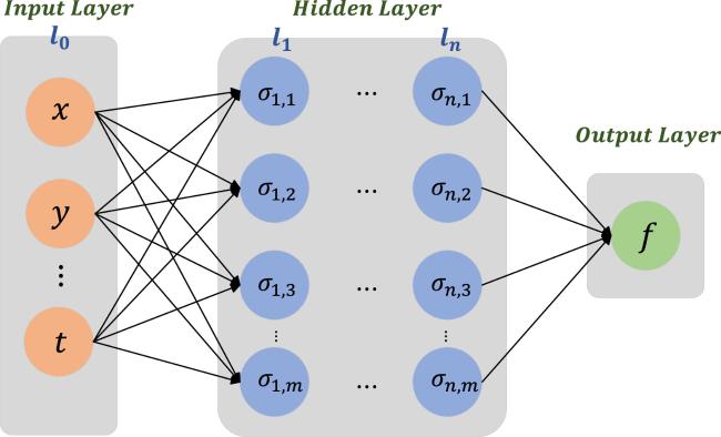
Figure 1. Neural network model for equation ( |
Step 1: By employing a bilinear transformation, the original equation is transformed into a bilinear form.
Step 2: Substituting the tensor formula equation (4 ) into equation (2 ) results in a complex equation concerning ωi,j and b.
Step 3: Coefficients of each term in the equation are gathered and required to be equal to zero, forming a nonlinear system concerning ωi,j and b.
Step 4: The corresponding parameter relations are obtained by solving the nonlinear system with Maple software.
Step 5: Substituting the solutions obtained in the previous step into equation (4 ) and through transformation, the exact analytical solution of the equation is obtained.
The models used in this paper are the single-layer model formed with n = 1 and the two-layer model formed with n = 2. Figure 2 illustrates some specific examples.
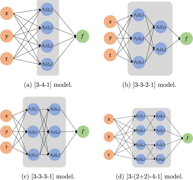
Figure 2. Different neural network models. |
3. Periodic solutions under the single-layer model
In this section, we will search for the periodic solutions using a single-layer network model. Figure 2(a) shows a schematic of the model with l0 = {x, y, t} as the input layer and 4 neurons in the single hidden layer. Letting ${F}_{1}(\xi )=\cosh (\xi )$, ${F}_{2}(\xi )=\cos (\xi )$, ${F}_{3}(\xi )=\sin (\xi )$ and ${F}_{4}(\xi )=\tanh (\xi )$, the associated tensor formula can be illustrated as:
$\begin{eqnarray}\begin{array}{rcl}f & = & {\omega }_{5,f}\cosh (t{\omega }_{t,1}+x{\omega }_{x,1}+y{\omega }_{y,1}+{b}_{1})\\ & & +\,{\omega }_{6,f}\cos (t{\omega }_{t,2}+x{\omega }_{x,2}+y{\omega }_{y,2}+{b}_{2})\\ & & +\,{\omega }_{7,f}\sin (t{\omega }_{t,3}+x{\omega }_{x,3}+y{\omega }_{y,3}+{b}_{3})\\ & & +\,{\omega }_{8,f}\tanh (t{\omega }_{t,4}+x{\omega }_{x,4}+y{\omega }_{y,4}+{b}_{4})+{b}_{5}.\end{array}\end{eqnarray}$
By substituting the set of tensor formula equation (6 ) into the bilinear equations equation (4 ) and aggregating the coefficients of all items and equating them to zero, an over-determined system of nonlinear equations can be derived. Twelve sets of real number solutions are obtained using Maple software, one of which is:6 ) yields the following analytic solution:
$\begin{eqnarray*}\mathrm{case}1:\left\{\begin{array}{l}{\omega }_{t,1}=-{c}_{2}{\omega }_{y,1},\,{\omega }_{t,2}={c}_{1}{\omega }_{x,3}^{3}-{c}_{2}{\omega }_{y,2},\,{\omega }_{t,3}={c}_{1}{\omega }_{x,3}^{3}+{c}_{2}{\omega }_{y,2},\,{\omega }_{x,1}=0,\\ {\omega }_{x,2}={\omega }_{x,3},\,{\omega }_{x,4}=0,\,{\omega }_{y,1}={\omega }_{y,1},\,{\omega }_{y,3}=-{\omega }_{y,2},\,{\omega }_{y,4}=-\tfrac{{\omega }_{t,4}}{{c}_{2}},\,{\omega }_{6,f}={\omega }_{7,f}\end{array}\right\}.\end{eqnarray*}$
Substituting case 1 into equation ( $\begin{eqnarray}\begin{array}{rcl}f & = & {\omega }_{5,f}\cosh \left(-{\omega }_{y,1}{\phi }_{2}+{b}_{1}\right)+{\omega }_{7,f}\sin \left({\phi }_{3}+{\omega }_{y,2}{\phi }_{2}+{b}_{3}\right)\\ & & +\,{\omega }_{7,f}\cos \left({\phi }_{3}-{\omega }_{y,2}{\phi }_{2}+{b}_{2}\right)\\ & & +\,{\omega }_{8,f}\tanh \left({\phi }_{1}\right)+{b}_{5},\\ & & \left\{\begin{array}{l}{\phi }_{1}=t{\omega }_{t,4}+{b}_{4}-\tfrac{y{\omega }_{t,4}}{{c}_{2}},\\ {\phi }_{2}={c}_{2}t-y,\\ {\phi }_{3}={c}_{1}t{\omega }_{x,3}^{3}+x{\omega }_{x,3}.\end{array}\right.\end{array}\end{eqnarray}$
To obtain the desired solution, it is necessary that the expressions within the cos, cosh, sin, and tanh functions are non-zero and that the coefficients preceding these functions are also non-zero. The periodic solution u for equation (1 ) can be derived through the transformation described in equation (3 ). To illustrate the dynamic characteristics of the result, we select certain parameters as ω5,f = 1, ω7,f = 1, ${\omega }_{8,f}=\tfrac{1}{2}$, ωx,3 = –4, ωy,1 = –1, ωy,2 = 2, ωt,4 = 1, b1 = 2, ${b}_{2}=-\tfrac{1}{2}$, b3 = 1, b4 = 2, b5 = 3, c1 = c2 = 1, then depict the corresponding three-dimensional figure and density figure as shown in figure 3.

Figure 3. (a) Three-dimensional figure of periodic solution with t = 0. (b) The density figure of (a). |
4. interaction solutions under the double-layer model
4.1. [3-3-2-1] lump solutions
The [3-3-2-1] neural network model shown by figure 2(b), which has three neurons in the first hidden layer and two neurons in the second hidden layer, will be used to obtain lump solutions. Letting Fi(ξ) = ξ(i = 1, 2, 3) and Fj(ξ) = ξ2(j = 4, 5), the following tensor formula is obtained:
$\begin{eqnarray}\begin{array}{rcl}f & = & {\omega }_{4,f}{\left({\omega }_{\mathrm{1,4}}{\xi }_{1}+{\omega }_{\mathrm{2,4}}{\xi }_{2}+{\omega }_{\mathrm{3,4}}{\xi }_{3}\right)}^{2}\\ & & +\,{\omega }_{5,f}{\left({\omega }_{\mathrm{1,5}}{\xi }_{1}+{\omega }_{\mathrm{2,5}}{\xi }_{2}+{\omega }_{\mathrm{3,5}}{\xi }_{3}\right)}^{2}+{b}_{6},\\ & & \left\{\begin{array}{l}{\xi }_{1}={\omega }_{t,1}t+{\omega }_{x,1}x+{\omega }_{y,1}y,\\ {\xi }_{2}={\omega }_{t,2}t+{\omega }_{x,2}x+{\omega }_{y,2}y,\\ {\xi }_{3}={\omega }_{t,3}t+{\omega }_{x,3}x+{\omega }_{y,3}y.\end{array}\right.\end{array}\end{eqnarray}$
A nonlinear algebraic system that consists of seven equations is obtained by substituting the above set of equations into the bilinear form of the equation and collecting the coefficients of all the items and letting their values be zero. Solving the equations using Maple software gives the following cases:8 ) yields equation (9 ):
$\begin{eqnarray*}\begin{array}{l}{\bf{case}}{\bf{1}}:\left\{\begin{array}{l}{\omega }_{\mathrm{1,4}}=0,\,{\omega }_{t,1}=-\tfrac{{\omega }_{\mathrm{2,5}}{\omega }_{t,2}+{\omega }_{\mathrm{3,5}}{\omega }_{t,3}}{{\omega }_{\mathrm{1,5}}},\,{\omega }_{x,2}=-\tfrac{{\omega }_{\mathrm{3,4}}{\omega }_{x,3}}{{\omega }_{\mathrm{2,4}}},\\ {\omega }_{y,1}=\tfrac{{c}_{2}{\omega }_{\mathrm{2,5}}{\omega }_{\mathrm{3,4}}{\omega }_{y,3}+{\omega }_{\mathrm{2,4}}{\omega }_{\mathrm{2,5}}{\omega }_{t,2}+{\omega }_{\mathrm{2,5}}{\omega }_{\mathrm{3,4}}{\omega }_{t,3}-{c}_{2}{\omega }_{\mathrm{2,4}}{\omega }_{\mathrm{3,5}}{\omega }_{y,3}}{{c}_{2}{\omega }_{\mathrm{1,5}}{\omega }_{\mathrm{2,4}}},\\ {\omega }_{y,2}=-\tfrac{{c}_{2}{\omega }_{\mathrm{3,4}}{\omega }_{y,3}+{\omega }_{\mathrm{2,4}}{\omega }_{t,2}+{\omega }_{\mathrm{3,4}}{\omega }_{t,3}}{{c}_{2}{\omega }_{\mathrm{2,4}}}\end{array}\right\};\\ {\bf{case}}{\bf{2}}:\left\{\begin{array}{l}{\omega }_{\mathrm{1,4}}=0,\,{\omega }_{y,1}=-\tfrac{{\omega }_{y,3}({\omega }_{\mathrm{2,4}}{\omega }_{\mathrm{3,5}}-{\omega }_{\mathrm{2,5}}{\omega }_{\mathrm{3,4}})}{{\omega }_{\mathrm{1,5}}{\omega }_{\mathrm{2,4}}},\,{\omega }_{y,2}=-\tfrac{{\omega }_{y,3}{\omega }_{\mathrm{3,4}}}{{\omega }_{\mathrm{2,4}}}\end{array}\right\};\\ {\bf{case}}{\bf{3}}:\left\{\begin{array}{l}{\omega }_{\mathrm{1,4}}=0,\,{\omega }_{\mathrm{2,4}}=0,\,{\omega }_{t,1}=-\tfrac{{\omega }_{\mathrm{2,5}}{\omega }_{t,2}+{\omega }_{\mathrm{3,5}}{\omega }_{t,3}}{{\omega }_{\mathrm{1,5}}},\,{\omega }_{x,3}=0,\\ {\omega }_{y,1}=-\tfrac{{c}_{2}{\omega }_{\mathrm{2,5}}{\omega }_{y,2}-{\omega }_{\mathrm{3,5}}{\omega }_{t,3}}{{c}_{2}{\omega }_{\mathrm{1,5}}},{\omega }_{y,3}=-\tfrac{{\omega }_{t,3}}{{c}_{2}}\end{array}\right\};\\ {\bf{case}}{\bf{4}}:\left\{\begin{array}{l}{\omega }_{\mathrm{1,4}}=0,\,{\omega }_{\mathrm{2,4}}=0,\,{\omega }_{y,1}=-\tfrac{{\omega }_{\mathrm{2,5}}{\omega }_{y,2}}{{\omega }_{\mathrm{1,5}}},\,{\omega }_{y,3}=0\end{array}\right\}.\end{array}\end{eqnarray*}$
Substituting the solution of case 1 into equation ( $\begin{eqnarray}\begin{array}{l}f={\omega }_{4,f}{\phi }_{1}^{2}{t}^{2}-\displaystyle \frac{2{\omega }_{4,f}{\phi }_{1}^{2}{yt}}{{c}_{2}}+\displaystyle \frac{{\omega }_{5,f}{\phi }_{2}^{2}{x}^{2}}{{\omega }_{2,4}^{2}}+\displaystyle \frac{{\omega }_{4,f}{\phi }_{1}^{2}{y}^{2}}{{c}_{2}^{2}}+{b}_{6},\\ \left\{\begin{array}{l}{\phi }_{1}={\omega }_{\mathrm{2,4}}{\omega }_{t,2}+{\omega }_{\mathrm{3,4}}{\omega }_{t,3},\\ {\phi }_{2}={\omega }_{\mathrm{1,5}}{\omega }_{\mathrm{2,4}}{\omega }_{x,1}+{\omega }_{\mathrm{2,4}}{\omega }_{\mathrm{3,5}}{\omega }_{x,3}-{\omega }_{\mathrm{2,5}}{\omega }_{\mathrm{3,4}}{\omega }_{x,3}.\end{array}\right.\end{array}\end{eqnarray}$
Using a bilinear transformation equation (3 ) of that solution yields a lump solution to equation (1 ). To avoid the occurrence of singularities in the solution, the parameters must meet certain conditions. When the parameters are set as ω4,f = 2, ω5,f = 2, ${\omega }_{x,1}=\tfrac{1}{2}$, ωx,3 = 2, ωt,2 = 1, ωt,3 = –1, ${\omega }_{\mathrm{1,5}}=\tfrac{1}{10}$, ω2,4 = 1, ω2,5 = 1, ${\omega }_{\mathrm{3,4}}=\tfrac{1}{5}$, ${\omega }_{\mathrm{3,5}}=\tfrac{1}{2}$, b6 = 1, c2 = 1, we obtain the lump solution, as shown in figure 4.
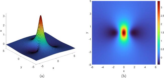
Figure 4. (a) Three-dimensional figure of lump solution with t = 0. (b) The density figure of (a). |
4.2. [3-3-3-1] interaction solutions between lump and one-stripe soliton
The [3-3-3-1] neural network model illustrated in figure 2(c), which consists of three neurons in the first hidden layer and the second hidden layer, will be used to find interaction solutions. Establishing Fi(ξ) = ξ(i = 1, 2, 3), Fj(ξ) = ξ2(j = 4, 6) and F5(ξ) = eξ, we derive the ensuing tensor formula:
$\begin{eqnarray}\begin{array}{rcl}f & = & {\omega }_{4,f}{\left({\omega }_{\mathrm{1,4}}{\xi }_{1}+{\omega }_{\mathrm{2,4}}{\xi }_{2}+{\omega }_{\mathrm{3,4}}{\xi }_{3}\right)}^{2}+{\omega }_{5,f}{{\rm{e}}}^{{\omega }_{\mathrm{1,5}}{\xi }_{1}+{\omega }_{\mathrm{2,5}}{\xi }_{2}+{\omega }_{\mathrm{3,5}}{\xi }_{3}}\\ & & +\,{\omega }_{6,f}{\left({\omega }_{\mathrm{1,6}}{\xi }_{1}+{\omega }_{\mathrm{2,6}}{\xi }_{2}+{\omega }_{\mathrm{3,6}}{\xi }_{3}\right)}^{2}+{b}_{7},\\ & & \left\{\begin{array}{l}{\xi }_{1}={\omega }_{t,1}t+{\omega }_{x,1}x+{\omega }_{y,1}y,\\ {\xi }_{2}={\omega }_{t,2}t+{\omega }_{x,2}x+{\omega }_{y,2}y,\\ {\xi }_{3}={\omega }_{t,3}t+{\omega }_{x,3}x+{\omega }_{y,3}y.\end{array}\right.\end{array}\end{eqnarray}$
Substituting equation (10 ) into equation (2 ) in the same way, collecting the coefficients of all the items to make them equal to zero, and solving the over-determined system using Maple software gives the following solutions:10 ) can obtain the following solution:
$\begin{eqnarray*}\begin{array}{l}{\bf{case}}{\bf{1}}:\left\{\begin{array}{l}{\omega }_{\mathrm{2,6}}=0,\,{\omega }_{x,3}=0,\,{\omega }_{t,1}=-{c}_{2}{\omega }_{y,1},\,{\omega }_{t,3}=-{c}_{2}{\omega }_{y,3},\\ {\omega }_{\mathrm{1,5}}=-\tfrac{{\omega }_{\mathrm{2,5}}{\omega }_{y,2}+{\omega }_{\mathrm{3,5}}{\omega }_{y,3}}{{\omega }_{y,1}},\\ {\omega }_{\mathrm{3,6}}=-\tfrac{{\omega }_{1,4}^{2}{\omega }_{4,f}{\omega }_{y,1}+{\omega }_{\mathrm{1,4}}{\omega }_{\mathrm{3,4}}{\omega }_{4,f}{\omega }_{y,3}+{\omega }_{1,6}^{2}{\omega }_{6,u}{\omega }_{y,1}}{{\omega }_{\mathrm{1,6}}{\omega }_{6,f}{\omega }_{y,3}},\\ {\omega }_{t,2}=\tfrac{{\left({\omega }_{\mathrm{2,5}}{\omega }_{x,1}{\omega }_{y,2}-{\omega }_{\mathrm{2,5}}{\omega }_{x,2}{\omega }_{y,1}+{\omega }_{\mathrm{3,5}}{\omega }_{x,1}{\omega }_{y,3}\right)}^{3}{c}_{1}}{{\omega }_{\mathrm{2,5}}{\omega }_{y,1}^{3}}-{c}_{2}{\omega }_{y,2}\end{array}\right\};\\ {\bf{case}}{\bf{2}}:\left\{\begin{array}{l}{\omega }_{\mathrm{1,4}}=-\tfrac{{\omega }_{\mathrm{3,4}}{\omega }_{y,3}}{{\omega }_{y,1}},\,{\omega }_{\mathrm{1,5}}=\tfrac{-{\omega }_{\mathrm{2,5}}{\omega }_{y,2}-{\omega }_{\mathrm{3,5}}{\omega }_{y,3}}{{\omega }_{y,1}},\,{\omega }_{\mathrm{1,6}}=-\tfrac{{\omega }_{\mathrm{3,6}}{\omega }_{y,3}}{{\omega }_{y,1}},\\ {\omega }_{t,2}=\tfrac{{\left[\left({\omega }_{x,1}{\omega }_{y,2}-{\omega }_{x,2}{\omega }_{y,1}\right){\omega }_{\mathrm{2,5}}+{\omega }_{\mathrm{3,5}}\left({\omega }_{x,1}{\omega }_{y,3}-{\omega }_{x,3}{\omega }_{y,1}\right)\right]}^{3}{c}_{1}+{\omega }_{\mathrm{2,5}}{\omega }_{t,1}{\omega }_{y,1}^{2}{\omega }_{y,2}}{{\omega }_{\mathrm{2,5}}{\omega }_{y,1}^{3}},\\ {\omega }_{\mathrm{2,4}}=0,\,{\omega }_{\mathrm{2,6}}=0,\,{\omega }_{t,3}=\tfrac{{\omega }_{t,1}{\omega }_{y,3}}{{\omega }_{y,1}}\end{array}\right\};\\ {\bf{case}}{\bf{3}}:\left\{\begin{array}{l}{\omega }_{\mathrm{2,4}}=0,\,{\omega }_{y,1}=0,\,{\omega }_{\mathrm{2,6}}=0,\,{\omega }_{t,1}=0,\,{\omega }_{\mathrm{2,5}}=-\tfrac{{\omega }_{\mathrm{3,5}}{\omega }_{y,3}}{{\omega }_{y,2}},\,{\omega }_{t,3}=-{c}_{2}{\omega }_{y,3},\\ {\omega }_{\mathrm{1,4}}=\tfrac{\left(-{\omega }_{3,4}^{2}{\omega }_{4,f}-{\omega }_{3,6}^{2}{\omega }_{6,f}\right){\omega }_{x,3}-{\omega }_{\mathrm{1,6}}{\omega }_{\mathrm{3,6}}{\omega }_{6,f}{\omega }_{x,1}}{{\omega }_{\mathrm{3,4}}{\omega }_{4,f}{\omega }_{x,1}},\\ {\omega }_{t,2}=\tfrac{{\left({\omega }_{\mathrm{1,5}}{\omega }_{x,1}{\omega }_{y,2}-{\omega }_{\mathrm{3,5}}{\omega }_{x,2}{\omega }_{y,3}+{\omega }_{\mathrm{3,5}}{\omega }_{x,3}{\omega }_{y,2}\right)}^{3}{c}_{1}}{{\omega }_{\mathrm{3,5}}{\omega }_{y,2}^{2}{\omega }_{y,3}}-{c}_{2}{\omega }_{y,2}\end{array}\right\};\\ {\bf{case}}{\bf{4}}:\left\{\begin{array}{l}{\omega }_{\mathrm{1,5}}=-\tfrac{{\omega }_{\mathrm{3,5}}{\omega }_{y,3}}{{\omega }_{y,1}},\,{\omega }_{\mathrm{2,5}}=0,\,{\omega }_{t,3}=-{c}_{2}{\omega }_{y,3},\,{\omega }_{x,3}=\tfrac{{\omega }_{x,1}{\omega }_{y,3}}{{\omega }_{y,1}},\,{\omega }_{t,1}=-{c}_{2}{\omega }_{y,1},\\ {\omega }_{t,2}=\tfrac{{c}_{2}\left[\left({\omega }_{\mathrm{1,4}}{\omega }_{y,1}+{\omega }_{\mathrm{3,4}}{\omega }_{y,3}\right)M{\omega }_{4,f}+\left({\omega }_{\mathrm{1,6}}{\omega }_{y,1}+{\omega }_{\mathrm{3,6}}{\omega }_{y,3}\right)N{\omega }_{6,f}\right]}{{\omega }_{\mathrm{2,4}}M{\omega }_{4,f}+{\omega }_{\mathrm{2,6}}N{\omega }_{6,f}},\\ {\omega }_{y,2}=\tfrac{-\left({\omega }_{\mathrm{1,4}}{\omega }_{y,1}+{\omega }_{\mathrm{3,4}}{\omega }_{y,3}\right)M{\omega }_{4,f}-\left({\omega }_{\mathrm{1,6}}{\omega }_{y,1}+{\omega }_{\mathrm{3,6}}{\omega }_{y,3}\right)N{\omega }_{6,f}}{{\omega }_{\mathrm{2,4}}M{\omega }_{4,f}+{\omega }_{\mathrm{2,6}}N{\omega }_{6,f}},\\ M={\omega }_{\mathrm{1,4}}{\omega }_{x,1}{\omega }_{y,1}+{\omega }_{\mathrm{2,4}}{\omega }_{x,2}{\omega }_{y,1}+{\omega }_{\mathrm{3,4}}{\omega }_{x,1}{\omega }_{y,3},\\ N={\omega }_{\mathrm{1,6}}{\omega }_{x,1}{\omega }_{y,1}+{\omega }_{\mathrm{2,6}}{\omega }_{x,2}{\omega }_{y,1}+{\omega }_{\mathrm{3,6}}{\omega }_{x,1}{\omega }_{y,3}\end{array}\right\}.\end{array}\end{eqnarray*}$
Substituting the solution in case 1 into equation ( $\begin{eqnarray}\begin{array}{rcl}f & = & {\omega }_{5,f}{{\rm{e}}}^{\tfrac{\left[{{tc}}_{1}{\phi }_{1}{\omega }_{x,1}({\phi }_{1}{\omega }_{x,1}-2{\omega }_{\mathrm{2,5}}{\omega }_{x,2}{\omega }_{y,1})+{\omega }_{y,1}^{2}\left({c}_{1}t{\omega }_{\mathrm{2,5}}^{2}{\omega }_{x,2}^{2}-x\right)\right]\left(-{\omega }_{\mathrm{2,5}}{\omega }_{x,2}{\omega }_{y,1}+{\phi }_{1}{\omega }_{x,1}\right)}{{\omega }_{y,1}^{3}}}\\ & & +\displaystyle \frac{{\omega }_{4,f}{\phi }_{2}{\left({c}_{2}t-y\right)}^{2}}{{\omega }_{1,6}^{2}{\omega }_{6,f}}+{\omega }_{x,1}^{2}{x}^{2}\left({\omega }_{1,4}^{2}{\omega }_{4,f}+{\omega }_{1,6}^{2}{\omega }_{6,f}\right)+{b}_{7},\\ & & \left\{\begin{array}{l}{\phi }_{1}={\omega }_{\mathrm{2,5}}{\omega }_{y,2}+{\omega }_{\mathrm{3,5}}{\omega }_{y,3},\\ {\phi }_{2}={\left({\omega }_{\mathrm{1,4}}{\omega }_{y,1}+{\omega }_{\mathrm{3,4}}{\omega }_{y,3}\right)}^{2}\left({\omega }_{1,4}^{2}{\omega }_{4,f}+{\omega }_{1,6}^{2}{\omega }_{6,f}\right).\end{array}\right.\end{array}\end{eqnarray}$
To render the dynamic properties of this solution more intuitively, we select appropriate parameters as ω4,f = 2, ω5,f = 2, ${\omega }_{x,1}=\tfrac{1}{2}$, ωx,3 = 2, ωt,2 = 1, ωt,3 = –1, ${\omega }_{\mathrm{1,5}}=\tfrac{1}{10}$, ω2,4 = 1, ω2,5 = 1, ${\omega }_{\mathrm{3,4}}=\tfrac{1}{5}$, ${\omega }_{\mathrm{3,5}}=\tfrac{1}{2}$, b6 = 1, c1 = c2 = 1, then generate visual representations at various time intervals as depicted in figure 5.
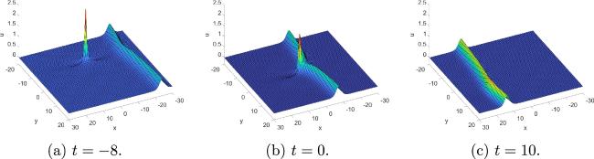
Figure 5. Three-dimensional figures of interaction solutions between lump and one-stripe soliton in different time. |
At time t = –8 in figure 5(a), the wave exhibits two distinct components: the lump wave and the stripe wave. Subsequently, the lump approaches the stripe, initiating an interaction between them. This interaction progresses over time, resulting in changes to the amplitudes, shapes, and velocities of both waves. By t = 10 in figure 5(c), the lump is engulfed or merged into the stripe, causing the stripe’s amplitude to exceed its original level. This exemplifies a fully non-elastic interaction between the two wave types.
4.3. [3-3-3-1] interaction solutions between lump and two-stripe solitons
Likewise, applying the [3-3-3-1] model depicted in figure 2(c), with Fi(ξ) = ξ(i = 1, 2, 3), Fj(ξ) = ξ2(j = 4, 6) and ${F}_{5}(\xi )=\cosh \xi $, the tensor formula can be formulated as follows :
$\begin{eqnarray}\begin{array}{rcl}f & = & {\omega }_{4,f}{\left({\omega }_{\mathrm{1,4}}{\xi }_{1}+{\omega }_{\mathrm{2,4}}{\xi }_{2}+{\omega }_{\mathrm{3,4}}{\xi }_{3}\right)}^{2}\\ & & +{\omega }_{5,f}\cosh ({\omega }_{\mathrm{1,5}}{\xi }_{1}+{\omega }_{\mathrm{2,5}}{\xi }_{2}+{\omega }_{\mathrm{3,5}}{\xi }_{3})\\ & & +\,{\omega }_{6,f}{\left({\omega }_{\mathrm{1,6}}{\xi }_{1}+{\omega }_{\mathrm{2,6}}{\xi }_{2}+{\omega }_{\mathrm{3,6}}{\xi }_{3}\right)}^{2}+{b}_{7},\\ & & \left\{\begin{array}{l}{\xi }_{1}={\omega }_{t,1}t+{\omega }_{x,1}x+{\omega }_{y,1}y,\\ {\xi }_{2}={\omega }_{t,2}t+{\omega }_{x,2}x+{\omega }_{y,2}y,\\ {\xi }_{3}={\omega }_{t,3}t+{\omega }_{x,3}x+{\omega }_{y,3}y.\end{array}\right.\end{array}\end{eqnarray}$
Similarly, substituting equation (12 ) into equation (2 ), collecting the coefficients of item to make it equal to zero, a set of nonlinear equations can be obtained and the following sets of cases are obtained after solving them with Maple software:12 ) can obtain the following solution:
$\begin{eqnarray*}\begin{array}{l}{\bf{case}}{\bf{1}}:\left\{\begin{array}{l}{\omega }_{\mathrm{1,4}}=0,\,{\omega }_{\mathrm{1,6}}=0,\,{\omega }_{x,3}=0,\,{\omega }_{t,2}=-{c}_{2}{\omega }_{y,2},\,{\omega }_{t,3}=-{c}_{2}{\omega }_{y,3},\\ {\omega }_{\mathrm{3,6}}=\tfrac{\left(-{\omega }_{2,4}^{2}{\omega }_{4,f}-{\omega }_{2,6}^{2}{\omega }_{6,f}\right){\omega }_{y,2}-{\omega }_{\mathrm{2,4}}{\omega }_{\mathrm{3,4}}{\omega }_{4,f}{\omega }_{y,3}}{{\omega }_{\mathrm{2,6}}{\omega }_{6,f}{\omega }_{y,3}},\,{\omega }_{y,1}=-\tfrac{{\omega }_{\mathrm{2,5}}{\omega }_{y,2}+{\omega }_{\mathrm{3,5}}{\omega }_{y,3}}{{\omega }_{\mathrm{1,5}}}\\ {\omega }_{t,1}=-{c}_{1}{\left({\omega }_{\mathrm{1,5}}{\omega }_{x,1}+{\omega }_{\mathrm{2,5}}{\omega }_{x,2}\right)}^{3}-\tfrac{{c}_{2}\left({\omega }_{\mathrm{2,5}}{\omega }_{y,2}+{\omega }_{\mathrm{3,5}}{\omega }_{y,3}\right)}{{\omega }_{\mathrm{1,5}}}\end{array}\right\};\\ {\bf{case}}{\bf{2}}:\left\{\begin{array}{l}{\omega }_{x,2}=0,\,{\omega }_{t,1}=-{c}_{2}{\omega }_{y,1},\,{\omega }_{t,2}=-{c}_{2}{\omega }_{y,2},\,{\omega }_{t,3}=-{c}_{2}{\omega }_{y,3},\\ {\omega }_{x,1}=-\tfrac{{\omega }_{\mathrm{3,5}}{\omega }_{x,3}}{{\omega }_{\mathrm{1,5}}},\,{\omega }_{\mathrm{2,5}}=-\tfrac{{\omega }_{\mathrm{1,5}}{\omega }_{y,1}+{\omega }_{\mathrm{3,5}}{\omega }_{y,3}}{{\omega }_{y,2}},\\ {\omega }_{\mathrm{2,4}}=\tfrac{{\omega }_{6,f}\left({\omega }_{\mathrm{1,5}}{\omega }_{\mathrm{3,6}}-{\omega }_{\mathrm{1,6}}{\omega }_{\mathrm{3,5}}\right)\left({\omega }_{\mathrm{1,6}}{\omega }_{y,1}+{\omega }_{\mathrm{2,6}}{\omega }_{y,2}+{\omega }_{\mathrm{3,6}}{\omega }_{y,3}\right)}{{\omega }_{4,f}{\omega }_{y,2}\left({\omega }_{\mathrm{1,4}}{\omega }_{\mathrm{3,5}}-{\omega }_{\mathrm{1,5}}{\omega }_{\mathrm{3,4}}\right)}-\tfrac{{\omega }_{\mathrm{1,4}}{\omega }_{y,1}+{\omega }_{\mathrm{3,4}}{\omega }_{y,3}}{{\omega }_{y,2}}\end{array}\right\};\\ {\bf{case}}{\bf{3}}:\left\{\begin{array}{l}{\omega }_{x,2}=0,\,{\omega }_{x,3}=0,\,{\omega }_{y,2}=0,\,{\omega }_{\mathrm{3,5}}=-\tfrac{{\omega }_{\mathrm{1,5}}{\omega }_{y,1}}{{\omega }_{y,3}},\\ {\omega }_{\mathrm{2,4}}=\tfrac{{c}_{1}{\omega }_{\mathrm{1,4}}{\omega }_{1,5}^{3}{\omega }_{x,1}^{3}{\omega }_{y,3}-\left({c}_{2}{\omega }_{y,3}+{\omega }_{t,3}\right)\left({\omega }_{\mathrm{1,4}}{\omega }_{y,1}+{\omega }_{\mathrm{3,4}}{\omega }_{y,3}\right){\omega }_{\mathrm{1,5}}+{\omega }_{\mathrm{1,4}}{\omega }_{\mathrm{2,5}}{\omega }_{t,2}{\omega }_{y,3}}{{\omega }_{y,3}{\omega }_{\mathrm{1,5}}{\omega }_{t,2}},\\ {\omega }_{\mathrm{2,6}}=\tfrac{{\omega }_{\mathrm{1,6}}{\omega }_{1,5}^{2}{c}_{1}{\omega }_{x,1}^{3}}{{\omega }_{t,2}}+\tfrac{{\omega }_{\mathrm{1,6}}{\omega }_{\mathrm{2,5}}}{{\omega }_{\mathrm{1,5}}}+\tfrac{{\omega }_{\mathrm{1,4}}{\omega }_{4,f}\left({\omega }_{\mathrm{1,4}}{\omega }_{y,1}+{\omega }_{\mathrm{3,4}}{\omega }_{y,3}\right)\left({c}_{2}{\omega }_{y,3}+{\omega }_{t,3}\right)}{{\omega }_{y,3}{\omega }_{\mathrm{1,6}}{\omega }_{6,f}{\omega }_{t,2}},\\ {\omega }_{\mathrm{3,6}}=\tfrac{\left(-{\omega }_{1,4}^{2}{\omega }_{4,f}-{\omega }_{1,6}^{2}{\omega }_{6,f}\right){\omega }_{y,1}-{\omega }_{\mathrm{1,4}}{\omega }_{\mathrm{3,4}}{\omega }_{4,f}{\omega }_{y,3}}{{\omega }_{\mathrm{1,6}}{\omega }_{6,f}{\omega }_{y,3}},\\ {\omega }_{t,1}=\tfrac{\left(-{c}_{1}{\omega }_{1,5}^{3}{\omega }_{x,1}^{3}-{\omega }_{\mathrm{2,5}}{\omega }_{t,2}\right){\omega }_{y,3}+{\omega }_{\mathrm{1,5}}{\omega }_{t,3}{\omega }_{y,1}}{{\omega }_{y,3}{\omega }_{\mathrm{1,5}}}\end{array}\right\}.\end{array}\end{eqnarray*}$
Substituting the solution in case 1 into equation ( $\begin{eqnarray}\begin{array}{rcl}f & = & {\omega }_{4,f}{c}_{2}^{2}{\phi }_{1}{t}^{2}-2{\omega }_{4,f}{c}_{2}{\phi }_{1}{yt}\\ & & +\,{\omega }_{x,2}^{2}\left({\omega }_{2,4}^{2}{\omega }_{4,f}+{\omega }_{2,6}^{2}{\omega }_{6,f}\right){x}^{2}+{\omega }_{4,f}{\phi }_{1}{y}^{2}\\ & & +\,{\omega }_{5,f}\cosh \left({\phi }_{2}\left(t{\phi }_{2}^{2}{c}_{1}-x\right)\right)+{b}_{7},\\ & & \left\{\begin{array}{l}{\phi }_{1}=\displaystyle \frac{1}{{\omega }_{2,6}^{2}{\omega }_{6,f}}{\left({\omega }_{\mathrm{2,4}}{\omega }_{y,2}+{\omega }_{\mathrm{3,4}}{\omega }_{y,3}\right)}^{2}\left({\omega }_{2,4}^{2}{\omega }_{4,f}+{\omega }_{2,6}^{2}{\omega }_{6,f}\right),\\ {\phi }_{2}={\omega }_{\mathrm{1,5}}{\omega }_{x,1}+{\omega }_{\mathrm{2,5}}{\omega }_{x,2}.\end{array}\right.\end{array}\end{eqnarray}$
By employing equation (3 ), a solution u for the equation is obtained. To provide a clear understanding of the dynamic characteristics of this solution, we select suitable parameters, such as ω4,f = 2, ω5,f = 1, ω6,f = 2, ${\omega }_{x,1}=\tfrac{1}{2}$, ${\omega }_{x,2}=\tfrac{1}{2}$, ${\omega }_{y,2}=\tfrac{1}{2}$, ${\omega }_{y,3}=\tfrac{1}{2}$, ωt,2 = 1, ω1,5 = 1, ω2,4 = 1, ω2,5 = 1, ω2,6 = 1, ω3,4 = 1, b7 = 1, c1 = 2, c2 = 1, and produce graphical depictions at different time intervals as illustrated in figure 6.
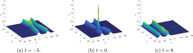
Figure 6. Three-dimensional of interaction solution between lump and two-stripe solitons in different time. |
As can be seen at the time t = –5 in figure 6(a), the wave exhibits a distinctive structure comprising two components: the lump wave and the two-stripe solitons wave. The lump emerges from one stripe and initiating a journey towards the opposite stripe. With time evolution, the magnitude fluctuates of lump wave notably reach the midpoint between the two-stripe solitons at t = 0. Subsequently, the lump wave progresses until it merges with the other stripe. This interaction process induces alterations in the amplitudes, shapes, and velocities of both waves.
4.4. [3-3-3-1] breather solutions
The [3-3-3-1] model for calculating the breather solutions is shown in figure 2(c). Letting Fi(ξ) = ξ(i = 1, 2, 3), F4(ξ) = e−ξ, ${F}_{5}(\xi )=\cos \xi $ and F6(ξ) = eξ, we obtain the corresponding tensor formula:
$\begin{eqnarray}\begin{array}{rcl}f & = & {\omega }_{4,f}{{\rm{e}}}^{-({\omega }_{\mathrm{1,4}}{\xi }_{1}+{\omega }_{\mathrm{2,4}}{\xi }_{2}+{\omega }_{\mathrm{3,4}}{\xi }_{3})}\\ & & +\,{\omega }_{5,f}\cos ({\omega }_{\mathrm{1,5}}{\xi }_{1}+{\omega }_{\mathrm{2,5}}{\xi }_{2}+{\omega }_{\mathrm{3,5}}{\xi }_{3})\\ & & +{\omega }_{6,f}{{\rm{e}}}^{{\omega }_{\mathrm{1,6}}{\xi }_{1}+{\omega }_{\mathrm{2,6}}{\xi }_{2}+{\omega }_{\mathrm{3,6}}{\xi }_{3}}+{b}_{7},\\ & & \left\{\begin{array}{l}{\xi }_{1}={\omega }_{t,1}t+{\omega }_{x,1}x+{\omega }_{y,1}y,\\ {\xi }_{2}={\omega }_{t,2}t+{\omega }_{x,2}x+{\omega }_{y,2}y,\\ {\xi }_{3}={\omega }_{t,3}t+{\omega }_{x,3}x+{\omega }_{y,3}y.\end{array}\right.\end{array}\end{eqnarray}$
Substituting equation (14 ) into equation (2 ) and collecting the coefficients of item to make it equal to zero, the resulting system of nonlinear equations will be solved using Maple software. The eligible solution is as follows: case 1:14 ), we can get the following solutions:
$\begin{eqnarray*}\left\{\begin{array}{l}{b}_{6}=0,\,{\omega }_{\mathrm{1,4}}=0,\,{\omega }_{\mathrm{2,4}}=0,N={\omega }_{\mathrm{1,5}}{\omega }_{x,1}+{\omega }_{\mathrm{2,5}}{\omega }_{x,2},\,L=3{\omega }_{x,2}^{2}{\omega }_{2,5}^{2}-3{\omega }_{x,3}^{2}\left({\omega }_{3,4}^{2}+{\omega }_{3,5}^{2}\right),\\ M=\tfrac{{\omega }_{x,2}^{3}{\omega }_{2,5}^{3}}{{\omega }_{\mathrm{1,5}}}-\tfrac{3{\omega }_{x,3}^{2}\left({\omega }_{3,4}^{2}+{\omega }_{3,5}^{2}\right){\omega }_{\mathrm{2,5}}{\omega }_{x,2}}{{\omega }_{\mathrm{1,5}}}-\tfrac{2{\omega }_{x,3}^{3}{\omega }_{\mathrm{3,5}}\left({\omega }_{3,4}^{2}+{\omega }_{3,5}^{2}\right)}{{\omega }_{\mathrm{1,5}}},\\ {\omega }_{6,f}=-\tfrac{{\omega }_{5,f}^{2}\left({\omega }_{\mathrm{1,5}}{\omega }_{x,1}+{\omega }_{\mathrm{2,5}}{\omega }_{x,2}+{\omega }_{\mathrm{3,5}}{\omega }_{x,3}\right)\left({\omega }_{\mathrm{1,5}}{\omega }_{y,1}+{\omega }_{\mathrm{2,5}}{\omega }_{y,2}+{\omega }_{\mathrm{3,5}}{\omega }_{y,3}\right)}{4{\omega }_{3,4}^{2}{\omega }_{4,f}{\omega }_{x,3}{\omega }_{y,3}},\\ {\omega }_{t,1}={c}_{1}\left({\omega }_{x,1}^{3}{\omega }_{1,5}^{2}+3{\omega }_{\mathrm{2,5}}{\omega }_{x,1}^{2}{\omega }_{x,2}{\omega }_{\mathrm{1,5}}+L{\omega }_{x,1}+M\right)-\tfrac{{c}_{2}\left({\omega }_{\mathrm{1,5}}{\omega }_{y,1}+{\omega }_{\mathrm{2,5}}{\omega }_{y,2}\right)}{{\omega }_{\mathrm{1,5}}}-\tfrac{{\omega }_{\mathrm{2,5}}{\omega }_{t,2}}{{\omega }_{\mathrm{1,5}}},\\ {\omega }_{t,3}={c}_{1}{\omega }_{x,3}\left[\left(-{\omega }_{3,4}^{2}+3{\omega }_{3,5}^{2}\right){\omega }_{x,3}^{2}+6{\omega }_{\mathrm{3,5}}{\omega }_{x,3}N+3{N}^{2}\right]-{c}_{2}{\omega }_{y,3}\end{array}\right\}.\end{eqnarray*}$
Substituting above case of parameters into the equation ( $\begin{eqnarray}\begin{array}{rcl}f & = & {\omega }_{5,f}\cos \left(-{c}_{1}t{\phi }_{1}^{3}+\left(3{c}_{1}t{\omega }_{3,4}^{2}{\omega }_{x,3}^{2}-x\right){\phi }_{1}+\left({c}_{2}t-y\right){\phi }_{2}\right)\\ & & -\,\displaystyle \frac{{\omega }_{5,f}^{2}{\phi }_{1}{\phi }_{2}}{4{\omega }_{3,4}^{2}{\omega }_{4,f}{\omega }_{x,3}{\omega }_{y,3}}{{\rm{e}}}^{{\phi }_{3}}+{\omega }_{4,f}{{\rm{e}}}^{-{\phi }_{3}},\\ & & \left\{\begin{array}{l}{\phi }_{1}={\omega }_{x,1}{\omega }_{\mathrm{1,5}}+{\omega }_{\mathrm{2,5}}{\omega }_{x,2}+{\omega }_{\mathrm{3,5}}{\omega }_{x,3},\\ {\phi }_{2}={\omega }_{\mathrm{1,5}}{\omega }_{y,1}+{\omega }_{\mathrm{2,5}}{\omega }_{y,2}+{\omega }_{\mathrm{3,5}}{\omega }_{y,3},\\ {\phi }_{3}=\left(-{c}_{1}{\omega }_{3,4}^{3}{\omega }_{x,3}^{3}+3{c}_{1}{\omega }_{\mathrm{3,4}}{\omega }_{x,3}{\phi }_{1}^{2}-{c}_{2}{\omega }_{\mathrm{3,4}}{\omega }_{y,3}\right)t+\left(x{\omega }_{x,3}+y{\omega }_{y,3}\right){\omega }_{\mathrm{3,4}}.\end{array}\right.\end{array}\end{eqnarray}$
The solution u of the equation (1 ) can be obtained by transform of equation (15 ). Selecting appropriate parameters as ω4,f = 4, ω5,f = 4, ωx,1 = 1, ${\omega }_{x,2}=\tfrac{6}{5}$, ${\omega }_{x,3}=\mbox{--}\tfrac{1}{2}$, ${\omega }_{y,1}=\tfrac{2}{3}$, ωy,2 = 2, ωy,3 = –3, ω1,5 = –1, ω2,5 = 2, ${\omega }_{\mathrm{3,4}}=\tfrac{1}{2}$, ω3,5 = 2, c1 = c2 = 1, we present the evolution behaviors of the breather solution seen in figure 7.
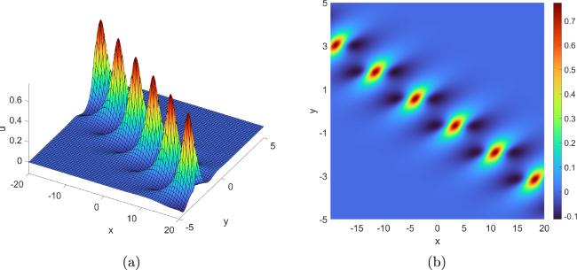
Figure 7. (a) Three-dimensional of breather solution with t = 0. (b) The density figure of (a). |
4.5. [3-(2+2)-4-1] periodic cross-rational solutions
The double-layer neural network model presented in this subsection is slightly different from the previous one. This model consists of four neurons in both the first and second hidden layers. However, the first hidden layer is divided into two separate networks for subsequent computation, as schematically illustrated in figure 2(d). Letting Fi(ξ) = ξ(i = 1, 2, 3, 4), Fj(ξ) = ξ2(j = 5, 6), ${F}_{7}(\xi )=\cosh \xi $ and ${F}_{8}(\xi )=\cos \xi $, the tensor formula can be expressed as follows [40]:
$\begin{eqnarray}\begin{array}{rcl}f & = & {\omega }_{5,f}{\left({\omega }_{\mathrm{1,5}}{\xi }_{1}+{\omega }_{\mathrm{2,5}}{\xi }_{2}\right)}^{2}\\ & & +\,{\omega }_{6,f}{\left({\omega }_{\mathrm{1,6}}{\xi }_{1}+{\omega }_{\mathrm{2,6}}{\xi }_{2}\right)}^{2}\\ & & +\,{\omega }_{7,f}\cosh \,({\omega }_{\mathrm{3,7}}{\xi }_{3}+{\omega }_{\mathrm{4,7}}{\xi }_{4})+{\omega }_{8,f}\cos ({\omega }_{\mathrm{3,8}}{\xi }_{3}+{\omega }_{\mathrm{4,8}}{\xi }_{4})+{b}_{9},\\ & & \left\{\begin{array}{l}{\xi }_{1}={\omega }_{t,1}t+{\omega }_{x,1}x+{\omega }_{y,1}y,\\ {\xi }_{2}={\omega }_{t,2}t+{\omega }_{x,2}x+{\omega }_{y,2}y,\\ {\xi }_{3}={\omega }_{t,3}t+{\omega }_{x,3}x+{\omega }_{y,3}y,\\ {\xi }_{4}={\omega }_{t,4}t+{\omega }_{x,4}x+{\omega }_{y,4}y.\end{array}\right.\end{array}\end{eqnarray}$
By substituting equation (16 ) into equation (2 ) and collecting coefficients to equate to zero, a series of nonlinear equations can be derived. Solving these equations using Maple software yields more than twenty sets of cases, one of solution is as follows:
$\begin{eqnarray*}{\bf{case}}{\bf{1}}:\left\{\begin{array}{l}{\omega }_{t,1}=-{c}_{2}{\omega }_{y,1},{\omega }_{y,2}=-\tfrac{{\omega }_{t,2}}{{c}_{2}},{\omega }_{x,2}=0,{\omega }_{x,4}=0,{\omega }_{y,3}=0,{\omega }_{y,4}=0,\\ {\omega }_{\mathrm{2,5}}=\tfrac{{c}_{2}{\omega }_{1,5}^{2}{\omega }_{5,f}{\omega }_{y,1}+{c}_{2}{\omega }_{1,6}^{2}{\omega }_{6,f}{\omega }_{y,1}-{\omega }_{\mathrm{1,6}}{\omega }_{\mathrm{2,6}}{\omega }_{6,f}{\omega }_{t,2}}{{\omega }_{\mathrm{1,5}}{\omega }_{5,f}{\omega }_{t,2}},\\ {\omega }_{\mathrm{4,7}}=-\tfrac{{\omega }_{\mathrm{3,7}}\left({c}_{1}{\omega }_{3,7}^{2}{\omega }_{x,3}^{3}+{\omega }_{t,3}\right)}{{\omega }_{t,4}},{\omega }_{\mathrm{4,8}}=\tfrac{{\omega }_{\mathrm{3,8}}\left({c}_{1}{\omega }_{3,8}^{2}{\omega }_{x,3}^{3}-{\omega }_{t,3}\right)}{{\omega }_{t,4}}\end{array}\right\}.\end{eqnarray*}$
By using the solution list above, we can obtain the following solution: $\begin{eqnarray}\begin{array}{rcl}f & = & {\omega }_{8,f}\cos \left({\omega }_{\mathrm{3,8}}{\omega }_{x,3}\left({c}_{1}t{\omega }_{3,8}^{2}{\omega }_{x,3}^{2}+x\right)\right)\\ & & +\,{\omega }_{7,f}\cosh \left({c}_{1}t{\omega }_{3,7}^{3}{\omega }_{x,3}^{3}-x{\omega }_{\mathrm{3,7}}{\omega }_{x,3}\right)\\ & & +\,{t}^{2}\phi -\displaystyle \frac{2{yt}\phi }{{c}_{2}}+{\omega }_{x,1}^{2}\left({\omega }_{1,5}^{2}{\omega }_{5,f}+{\omega }_{1,6}^{2}{\omega }_{6,f}\right){x}^{2}+\displaystyle \frac{{y}^{2}\phi }{{c}_{2}^{2}}+{b}_{9},\end{array}\end{eqnarray}$
with $\phi =\tfrac{{\omega }_{6,f}{\left({c}_{2}{\omega }_{\mathrm{1,6}}{\omega }_{y,1}-{\omega }_{\mathrm{2,6}}{\omega }_{t,2}\right)}^{2}\left({\omega }_{1,5}^{2}{\omega }_{5,f}+{\omega }_{1,6}^{2}{\omega }_{6,f}\right)}{{\omega }_{1,5}^{2}{\omega }_{5,f}}$.By using the transformation equation (3 ), we can derive the solution u. Setting the parameters appropriately as ω5,f = 1, ω6,f = 1, ω7,f = 1, ω8,f = − 1, ωx,1 = 3, ωx,3 = 2, ωy,1 = 1, ωt,2 = 1, ${\omega }_{\mathrm{1,5}}=\tfrac{1}{2}$, ${\omega }_{\mathrm{1,6}}=\tfrac{3}{10}$, ω2,6 = 1, ${\omega }_{\mathrm{3,7}}=\tfrac{3}{10}$, ω3,8 = 3, b9 = 1, c1 = 1, c2 = 2, the dynamics of this solution are illustrated in figure 8.
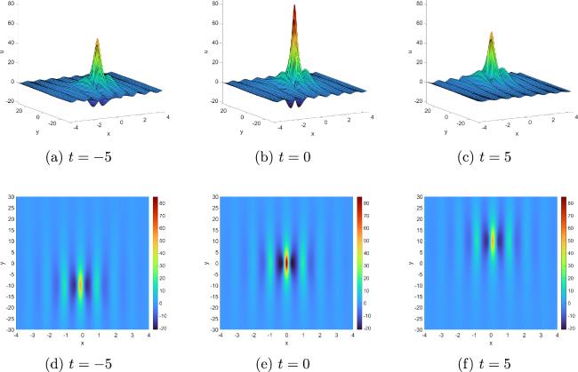
Figure 8. (a),(b),(c) Three-dimensional of periodic cross-rational solutions in different time. (d),(e),(f) The density figures of (a)(b)(c), respectively. |
As shown in figure 8, the solution exhibits repeating wave-like patterns coupled with sharp peaks. The periodic character of this solution depicts the system’s regular oscillation pattern, whereas the sharp features highlight localized alterations. This type of solution is also suitable for modeling various physical phenomena [40]. It can represent oscillatory flows with abrupt changes in velocity or pressure fields in fluid dynamics.
5. Conclusion
In this paper, we employ a novel method called BNNM, inspired by Hirota’s bilinear method and neural network models, to seek the exact solution of a generalized (2+1)-dimensional Hirota bilinear equation. Based on the method, both single-layer models and double-layer models are used to compute various types of solutions. Using different activation functions and conducting symbolic operations with Maple software, we found periodic solutions utilizing the [3-4-1] model. Additionally, we investigate lump solutions and their interactions with one-stripe and two-stripe solitons, as well as breather solutions, employing the [3-3-2-1] and [3-3-3-1] model. These solutions possess completely new analytical forms, distinguishing them from those previously reported in the literature. By researching its kinetic properties, we discovered that during the interaction between the lump and one-stripe soliton, the lump gradually approaches the stripe and is eventually engulfed. While during the interaction between the lump and two-stripe solitons, the lump gradually shifts from one stripe to the other, reaching its peak at the midpoint and ultimately being absorbed. Moreover, we introduce the [3-(2+2)-4-1] model, which involves dividing one of the hidden layer’s layers into two parts and subsequently incorporating them into subsequent operations. This approach yields the periodic cross-rational solutions. To the best of our knowledge, this type of solution has not been previously reported in the study of the (2 + 1)-dimensional Hirota bilinear equation. The dynamic characteristics of these solutions are analyzed by generating three-dimensional and density figures.
Theoretically, this method can be applied to all equations that allow for bilinear variation. By changing the activation function, different types of solutions can be obtained, as well as more exact solutions. However, as the order increases, the corresponding computational process becomes increasingly complex and places greater demands on the design of the model. In the future, improvements to the model can be pursued by increasing the number of hidden layers, exploring alternative activation functions, and employing more diverse layering strategies. Moreover, we can employ new techniques, such as bilinear residual network methods, which will help us apply our approach to a broader range of differential equations. By adopting these advanced methods, we aim to study other complex equations and enrich the scope and applications of our work.