We investigate dark solitons lying on elliptic function background in the defocusing Hirota equation with third-order dispersion and self-steepening terms. By means of the modified squared wavefunction method, we obtain the Jacobi’s elliptic solution of the defocusing Hirota equation, and solve the related linear matrix eigenvalue problem on elliptic function background. The elliptic N-dark soliton solution in terms of theta functions is constructed by the Darboux transformation and limit technique. The asymptotic dynamical behaviors for the elliptic N-dark soliton solution as t → ± ∞ are studied. Through numerical plots of the elliptic one-, two- and three-dark solitons, the amplification effect on the velocity of elliptic dark solitons, and the compression effect on the soliton spatiotemporal distributions produced by the third-order dispersion and self-steepening terms are discussed.
Xin Wang, Jingsong He. Dark solitons on elliptic function background for the defocusing Hirota equation[J]. Communications in Theoretical Physics, 2025, 77(3): 035003. DOI: 10.1088/1572-9494/ad84be
1. Introduction
The nonlinear Schrödinger (NLS) equation plays a fundamental role in a wide range of physical branches such as nonlinear optics [1, 2], water waves [3], nonlinear quantum field theory [4], plasma physics [5] and Bose–Einstein condensates [6]. Particularly in nonlinear optics, it can be used to describe the propagation of picosecond optical solitons in fibers. Nonetheless, in order to model the subpicosecond or femtosecond optical solitons, one should not be confined to the standard NLS description and the higher-order effects become important.
One version of the generalized NLS equation with higher-order effects was proposed by Hasegawa and Kodama [7], as
Here α1, α2, β1, β2, β3 are real constants and denote the group velocity dispersion, Kerr nonlinearity, third-order dispersion, self-steepening and stimulated Raman scattering, respectively. In the viewpoint of mathematics, four integrable cases for equation (1) have received widespread concern during the past few years, i.e., the derivative NLS equation [8] (β1: β2: β3 = 0: 1: 1), the Chen-Lee-Liu equation [9] (β1: β2: β3 = 0: 1: 0), the Hirota equation [10] (β1: β2: β3 = 1: 6σ: 0) and the Sasa–Satsuma equation [11] (β1: β2: β3 = 1: 6σ: 3σ).
Obtaining explicit localized wave solutions including soliton, breather and rogue wave solutions, and exploring their dynamical behaviors have been two important tasks for the investigations of integrable systems. Especially, localized wave solutions under fluctuating periodic backgrounds have drawn a surge of research activities within the last decades. For instance, based on the modified squared wavefunction (MSW) approach [12–15] and Darboux transformation (DT), the single-breather solution of the focusing NLS equation on the elliptic function background was obtained in [16]. This solution can be expressed by Jacobi’s elliptic functions, Weierstrass’ functions or theta functions. Meanwhile, the one-dark soliton solution of the defocusing NLS equation and the one-dark-bright soliton solution of the coupled NLS equations on the cnoidal wave background were considered by the same author [17, 18]. Furthermore, the soliton-cnoidal wave interaction solutions of the Kortewet–de Vries (KdV) equation and the focusing NLS equation were constructed by the nonlocal symmetry reduction method [19, 20] or the consistent Riccati expansion method [21]. More recently, the multi-breather and rogue wave solutions on elliptic function backgrounds have been paid increasingly considerable attention. The higher-order rogue wave solutions of the focusing NLS equation on cnoidal and dnoidal function backgrounds were illustrated through the numerical method and DT [22]. The generalized first-order rogue wave solution of the focusing NLS equation moving on a fluctuating (elliptic function) background was explicitly presented by the MSW approach and DT [23]. Subsequently, the first- and the second-order rogue wave solutions of the focusing NLS equation and the modified KdV equation on the elliptic function background were constructed by combining the nonlinearization of the Lax pair with DT [24, 25]. Besides, the multi-breather and higher-order rogue wave solutions of the focusing NLS equation and the multi-dark soliton solution of the defocusing NLS equation on an elliptic function background were constructed with the help of the MSW approach together with DT [26, 27]. In addition, the breather and rogue wave solutions of the higher-order NLS equations and other generalized integrable systems have also been widely investigated by many authors [28–31].
As is motioned above, by choosing α1 = α2/(2σ) = α, β1 = β2/(6σ) = β and β3 = 0 in equation (1), one obtains the Hirota equation [10]
where u(x, t) is the complex-valued envelope, α and β are two constants, σ = 1 denotes the focusing case and σ = − 1 denotes the defocusing case. When α = 1, β = 0, equation (2) reduces to the standard NLS equation, and when α = 0, β = 1 it becomes the complex modified KdV equation [32]. Until now, the bright soliton solution on zero background as well as the breather and rogue wave solutions on plane-wave or elliptic function background for the focusing Hirota equation have been studied in [10, 33–36]. It has been demonstrated that the third-order dispersion and self-steepening terms with respect to β could produce the compression effect on the spatiotemporal distributions of breathers and rogue waves [33]. Particularly, the state transitions between breathers/rogue waves and W-shaped solitons could be induced by higher-order effects [35, 36]. It has been found that these transitions occur in a modulation stability region with low-frequency perturbations related to the parameter β. Recently, the multi-dark soliton solutions on the plane-wave background and the elastic or inelastic collisions among these dark solitons for the defocusing Hirota equation were discussed in [37, 38].
In this paper, we study the multi-dark soliton solutions arising on the elliptic function background and discuss their asymptotic dynamical behaviors for the defocusing Hirota equation. This paper is organized as follows. In section 2, on the basis of the MSW approach, we derive Jacobi’s elliptic solution of the defocusing Hirota equation and give the fundamental solution of the related linear matrix eigenvalue problem on Jacobi’s elliptic function background. In section 3, we present the elliptic N-dark soliton solution in terms of theta functions by utilizing the DT together with the limit technique [39–44]. In section 4, we display the numerical plots of the elliptic one-, two- and three-dark solitons, and discuss the asymptotic dynamical behaviors for the elliptic N-dark soliton solution as t → ±∞. Interestingly, we show that the third-order dispersion and self-steepening terms in the defocusing Hirota equation can exert the amplification effect on the velocity of elliptic dark solitons, and the compression effect on the soliton spatiotemporal distributions. Section 5 contains our conclusions.
2. The elliptic solution of the defocusing Hirota equation
In this section, by means of the standard MSW approach [12–15], we first construct Jacobi’s elliptic solution of the defocusing Hirota equation and further derive the fundamental solution of the corresponding linear matrix eigenvalue problem on Jacobi’s elliptic function background. The MSW approach is based on our starting point and is the following 2 × 2 linear matrix eigenvalue problem [45]
As V is a polynomial of λ with matrix coefficients, it is convenient to provide the explicit expressions Vi (i = 0, 1, 2, 3) in equation (4). The straightforward verification of the compatibility condition Ut − Vx + UV − VU = 0 for equation (3a) can give rise to equation (2) with σ = − 1. Suppose equation (3a) has two basic solutions ${{\rm{\Phi }}}_{1}={({\psi }_{1},{\varphi }_{1})}^{{\rm{T}}}$ and ${\widetilde{{\rm{\Phi }}}}_{1}={({\widetilde{\psi }}_{1},{\widetilde{\varphi }}_{1})}^{{\rm{T}}}$, we can build a squared wavefunction in the form of
It is ready to check that P(λ) = f2 − gh is independent of x and t and is only a function on λ. It is known that the one-phase periodic solution corresponds to a fourth-degree polynomial, and the two-phase periodic solution is related to a sixth-degree polynomial [12]. Consequently, to derive the one-phase periodic solution, we introduce
At this point, let $W=x+\left(\alpha {s}_{1}+\displaystyle \frac{3}{2}\beta {s}_{1}^{2}-2\beta {s}_{2}\right)t$, then equations (14) and (15) can be rewritten as
From equations (10) and (11), we know that f1 is a constant and is related to the moving velocity of the elliptic function background (29). For simplicity, we set f1 = 0 in the rest of this paper and the case of f1 ≠ 0 can be similarly treated. At this very point, the quantity η = ∣u∣2 (27) and the one-phase periodic solution (29) can be simplified as
In the following, we proceed to the calculations of ${({\psi }_{1},{\varphi }_{1})}^{{\rm{T}}}$ and ${({\widetilde{\psi }}_{1},{\widetilde{\varphi }}_{1})}^{{\rm{T}}}$ associated with equation (3a) with the aid of the MSW approach [12–15]. To this end, we denote χ = φ1/ψ1, then equation (5) turns into
in which the ± sgn represent two sets of the solutions for equation (3a). We next take the + sgn to derive the first set of the solution ${({\psi }_{1},{\varphi }_{1})}^{{\rm{T}}}$, and the second set of the solution ${({\widetilde{\psi }}_{1},{\widetilde{\varphi }}_{1})}^{{\rm{T}}}$ related to the-sgn can be similarly presented. To this end, by using equations (9)–(11) and (35), we rewrite equation (3a) as
which yields that C2/C1 = i, and without loss of generality we choose C1 = 1 and C2 = i. At this moment, we can end up with the fundamental solution of equation (3a) on the elliptic function background (30), viz.,
In this section, we shall construct the elliptic N-dark soliton solution in terms of theta functions for the defocusing Hirota equation. Firstly, we introduce the parameterization
Furthermore, we should parameterize the spectral curve by taking λ = μ(2iK(z − l)) and $\sqrt{P}=\tfrac{1}{4K}\tfrac{{\rm{d}}\mu }{{\rm{d}}{z}}$, then it yields that
Here ${{\rm{\Phi }}}_{j}={({\psi }_{j},{\varphi }_{j})}^{{\rm{T}}}$ (j = 1, 2, ⋯ ,N) are N basic solutions of equation (3a) at λ = λj. Being different from the classical DT of the focusing case [33], in order to obtain the multi-dark soliton solution, one should use the limit technique of the above DT and restrict ${\lambda }_{j}\in {\mathbb{R}}$, i.e. ${\lambda }_{j}\to {\lambda }_{j}^{* }$. Therefore, by using
we can set ${\vartheta }_{4}({\rm{i}}({z}_{j}+{z}_{j}^{* }))=0$, namely, ${\mathfrak{R}}({z}_{j})=\pm \tfrac{K^{\prime} }{4K}$, then ${\lambda }_{j}-{\lambda }_{j}^{* }$ equals to zero. In this circumstance, letting ${{\rm{\Phi }}}_{j}={\rm{\Phi }}{({z}_{j})(1,{a}_{j}{\vartheta }_{4}({\rm{i}}({z}_{j}+{z}_{j}^{* })))}^{T}$, here aj (j = 1, 2, ⋯ ,N) are free constants, and utilizing the limit technique we can put forward the elliptic N-dark soliton solution
with δjl being the Kronecker delta function and ${\widehat{a}}_{j}={\mathfrak{I}}({a}_{j}){{\rm{e}}}^{\pi K^{\prime} /(4K)}$.
4. Dynamics and asymptotic behaviors of the elliptic dark solitons
In this section, we shall discuss the dynamics of the elliptic one-, two- and three-dark soliton solutions and their asymptotic dynamical behaviors. Firstly, we denote
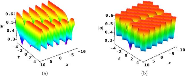
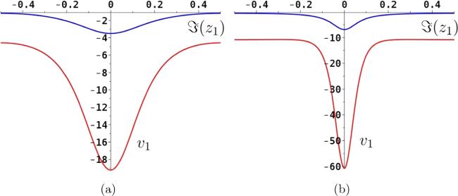
The evolution plots of the elliptic one-dark soliton solution are shown in figure 1. The velocity of the elliptic one-dark soliton is v1, and it is shown in figure 2 that, the parameter β which represents the strength of the third-order dispersion and self-steepening terms can exert an amplification effect on the soliton velocity. Specifically, when the value of β increases, the absolute value of the velocity would also be enlarged. The maximum value of ∣v1∣ occurs ${\mathfrak{I}}({z}_{1})=n$ and the minimum value of it occurs ${\mathfrak{I}}({z}_{1})=\tfrac{1}{2}+n$ (n = 0, ± 1, ± 2, ⋯ ). In addition, for the fixed time t, we have the asymptotic solutions
Figure 2. The velocity of the elliptic one-dark soliton v1 versus ${\mathfrak{I}}({z}_{1})$ with $\alpha =1,l=\tfrac{1}{10},{\widehat{a}}_{1}=1,{z}_{1}=-\tfrac{K^{\prime} }{4K}+\tfrac{{\rm{i}}}{15}$ for $\beta =\tfrac{1}{20}$ (blue solid line) and β = 2 (red solid line): (a) $k=\tfrac{1}{2}$ and (b) $k=\tfrac{9}{10}$.
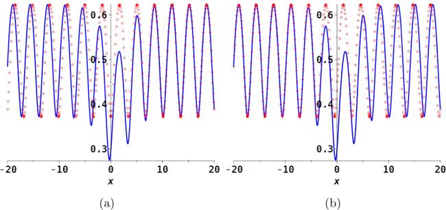
Figure 3. The asymptotic behaviors of the elliptic one-dark soliton solution at t = 0. (a) The asymptotic behavior for x→ + ∞ given by $| u{\left[1\right]}_{+}| $ (red dashed line) and (b) the asymptotic behavior for x→ − ∞ given by $| u{\left[1\right]}_{-}| $ (red dashed line). The blue solid line represents ∣u[1]∣ at t = 0. The parameters are the same as figure 1(a).
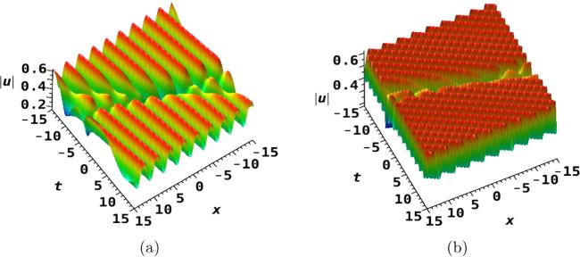
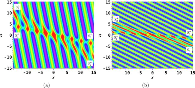
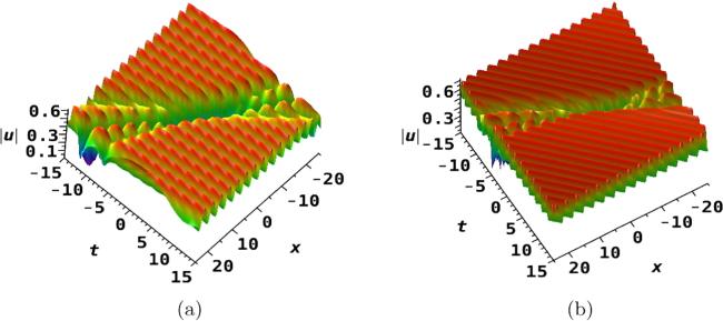
In what follows, for N = 2 in equation (65), we can obtain the elliptic two-dark soliton solution. Dynamics of the elliptic two-dark soliton solution and their density plots are shown in figures 4 and 5, respectively. Interestingly, it is shown that the compression effect on the soliton spatiotemporal distributions is produced by the third-order dispersion and self-steepening terms with respect to the parameter β. The included angle between the solitons S1 and S2 in figure 5(a) for $\beta =\tfrac{1}{10}$ is $\arctan (0.3222)\,\approx 17.86^\circ $, while in figure 5(b) for β = 1 it decreases to$\arctan (0.1916)\approx 10.85^\circ $.
is the phase difference after the collisions of the two elliptic dark solitons, and the dynamics of the above asymptotic solutions of u[2] for t → ± ∞along the trajectories θi (i = 1,2) are displayed in figures 6 and 7, respectively.
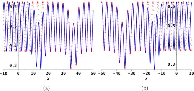
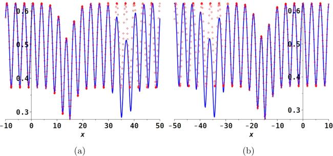
Figure 6. The asymptotic behaviors of the elliptic two-dark soliton solution. (a) The asymptotic behavior given by $| u{\left[2\right]}_{{{\rm{S}}}_{1}^{-}}| $ at t = −10 (red dashed line) and (b) the asymptotic behavior given by $| u{\left[2\right]}_{{{\rm{S}}}_{1}^{+}}| $ at t = 10 (red dashed line). The blue solid line represents ∣u[2]∣ at (a) t = −10 and (b) t = 10. The parameters are the same as figure 4(a).
Figure 7. The asymptotic behaviors of the elliptic two-dark soliton solution. (a) The asymptotic behavior given by $| u{\left[2\right]}_{{{\rm{S}}}_{2}^{-}}| $ at t = −10 (red dashed line) and (b) the asymptotic behavior given by $| u{\left[2\right]}_{{{\rm{S}}}_{2}^{+}}| $ at t = 10 (red dashed line). The blue solid line represents ∣u[2]∣ at (a) t = −10 and (b) t = 10. The parameters are the same as figure 4(a).
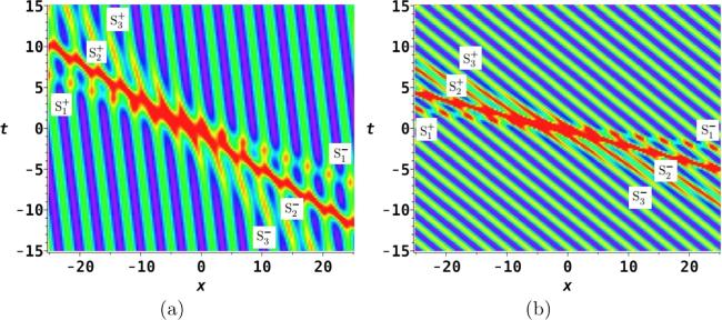
Analogously, the elliptic three-dark soliton solution can be provided with the aid of N = 3 in equation (65). Figures 8 and 9 exhibit the dynamics of the elliptic three-dark soliton solution and their density plots, respectively. Obviously, the compression effect produced by the parameter β can also be illustrated. It is numerically calculated that the included angle between the solitons S1 and S2 and the included angle between the solitons S2 and S3 in figure 9(a) for $\beta =\tfrac{1}{10}$ are $\arctan (0.1661)\approx 9.43^\circ $ and $\arctan (0.1481)\approx 8.43^\circ $, respectively, but they are compressed to $\arctan (0.1024)\approx 5.85^\circ $ and $\arctan (0.0875)\approx 5.00^\circ $ in figure 9(b) for β = 1.
For illustration, figures 10–12 show the dynamics of the asymptotic solutions of u[3] for t → ± ∞along the trajectories θi (i = 1, 2, 3), respectively.
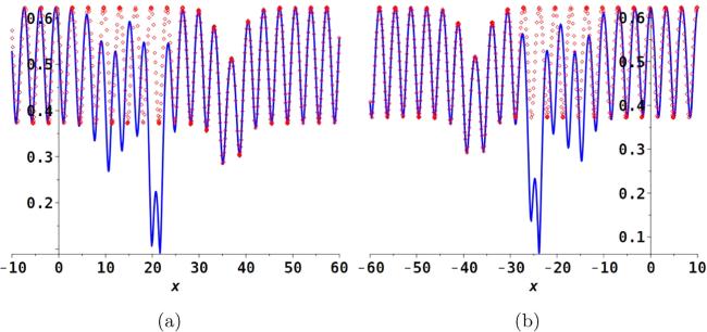
Figure 10. The asymptotic behaviors of the elliptic three-dark soliton solution. (a) The asymptotic behavior given by $| u{\left[3\right]}_{{{\rm{S}}}_{1}^{-}}| $ at t = −10 (red dashed line) and (b) the asymptotic behavior given by $| u{\left[3\right]}_{{{\rm{S}}}_{1}^{+}}| $ at t = 10 (red dashed line). The blue solid line represents ∣u[3]∣ at (a) t = −10 and (b) t = 10. The parameters are the same as figure 8(a).
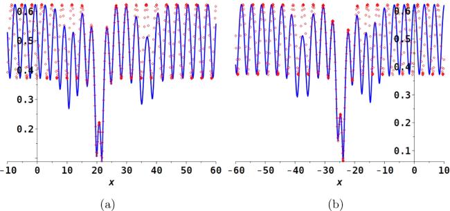
Figure 11. The asymptotic behaviors of the elliptic three-dark soliton solution. (a) The asymptotic behavior given by $| u{\left[3\right]}_{{{\rm{S}}}_{2}^{-}}| $ at t = −10 (red dashed line) and (b) the asymptotic behavior given by $| u{\left[3\right]}_{{{\rm{S}}}_{2}^{+}}| $ at t = 10 (red dashed line). The blue solid line represents ∣u[3]∣ at (a) t = −10 and (b) t = 10. The parameters are the same as figure 8(a).
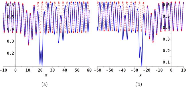
Figure 12. The asymptotic behaviors of the elliptic three-dark soliton solution. (a) The asymptotic behavior given by $| u{\left[3\right]}_{{{\rm{S}}}_{3}^{-}}| $ at t = −10 (red dashed line) and (b) the asymptotic behavior given by $| u{\left[3\right]}_{{{\rm{S}}}_{3}^{+}}| $ at t = 10 (red dashed line). The blue solid line represents ∣u[3]∣ at (a) t = −10 and (b) t = 10. The parameters are the same as figure 8(a).
Finally, if ${\theta }_{{iR}}=\mathrm{constant}$ (1 ≤ i ≤ N), the asymptotic analysis for the elliptic N-dark soliton solution can be put forward. We conclude that:
In conclusion, we have considered dark solitons arising on elliptic function background and their asymptotic behaviors for the defocusing Hirota equation, which contains the third-order dispersion and self-steepening terms and can be applied to simulate the propagation of subpicosecond or femtosecond optical solitons in fibers. The main results of this paper can be listed as follows:
•
On the basis of the MSW approach, we have obtained Jacobi’s elliptic solution (30) of the defocusing Hirota equation, and particularly, we have constructed the fundamental solution (47) of the linear matrix eigenvalue problem associated with the defocusing Hirota equation on the initial elliptic solution.
•
We have derived the elliptic N-dark soliton solution (65) in terms of theta functions by means of the DT and limit technique for the defocusing Hirota equation. The asymptotic analysis for the elliptic N-dark soliton solution along the fixed trajectories has been performed in equations (85)–(88). The numerical plots of the elliptic one-, two- and three-dark solitons and their asymptotic behaviors have been shown, see figures 1, 3, 4–12.
•
The amplification effect on the velocity of elliptic dark solitons and the compression effect produced by the parameter β which denotes the strength of the third-order dispersion and self-steepening terms have been considered in detail. It has been demonstrated that, when the value of β increases, the absolute value of the soliton velocity would also be amplified, see figure 2. Moreover, the compression effect on the soliton spatiotemporal distributions induced by the parameter β is discussed, see figures 5 and 9.
Finally, we anticipate that the results presented in this paper may help to understand the complicated dark solitons on fluctuating periodic background described by the higher-order NLS equations with third-order dispersion and self-steepening terms in nonlinear optics, water waves, and so on.
Acknowledgments
The work was supported by the National Natural Science Foundation of China (Grant No. 12326304, 12326305, 12071304), the Shenzhen Natural Science Fund (the Stable Support Plan Program) (Grant No. 20220809163103001), the Natural Science Foundation of Henan Province (Grant No. 232300420119), the Excellent Science and Technology Innovation Talent Support Program of ZUT (Grant No. K2023YXRC06) and Funding for the Enhancement Program of Advantageous Discipline Strength of ZUT (2022).
CRediT authorship contribution statement
XW: Conceptualization, Methodology, Design, Formal analysis, Software, Validation, Writing-original draft, Writing-review and editing. JH: Software, Writing-review and editing.
Declaration of competing interest
The authors declare that they have no known competing financial interests.
HasegawaA, TappertF1973 Transmission of stationary nonlinear optical pulses in dispersive dielectric fibres II. Normal dispersion Appl. Phys. Lett.23 171 172
KonotopV V, PaccianiP2005 Collapse of solutions of the nonlinear Schrödinger equation with a time-dependent nonlinearity: application to Bose-Einstein condensates Phys. Rev. Lett.94 240405
FengB F, LingL M, TakahashiD A2019 Multi-breather and high-order rogue waves for the nonlinear Schrödinger equation on the elliptic function background Stud. Appl. Math.144 46 101
SinthujaN, ManikandanK, SenthilvelanM2021 Formation of rogue waves on the periodic background in a fifth-order nonlinear Schrödinger equation Phys. Lett. A415 127640
ZhangY, ZhangH Q, WeiY C, LiuR2023 Nonlinear mechanism of breathers and rogue waves for the Hirota equation on the elliptic function background Nonlinear Dyn.111 6639 6658


