


Gross–Pitaevskii equation $\qquad$ GPE
Generalized Kudryashov scheme GKS
Haar Wavelet Numerical scheme HWNS
1. Introduction
Generally, according to the soliton theory, the soliton is a solitary wave that has constant shape and speed that can be realized by cancelation of the nonlinear effect and the dispersion effect [1–5], for example, the static and dynamic characteristics of polarization Bose–Einstein condensates. This can be done through experimental studies of coherent nonlinear dynamics [6–11] in which these properties can be represented by the Gross–Pitaevskii equation, which is one of the forms of the nonlinear Schrodinger equation. The study of the soliton in polarization condensates is among the hottest topics and aims to obtain novel scenarios in which the combined effects of dissipation and nonlinearity on the nonlinear phenomena will disappear with an emphasis on capturing the non-equilibrium nature of the soliton with no analog in the static counterpart [12–21]. A number of dark solitons created by non-resonantly pumped excitation in a polarization condensate appear as the result of a moving defect that is dependent on the pump power [16]. The dynamics of two dark solitons in a polarization condensate under non-resonant pumping that can be described by the Gross–Pitaevskii equations coupled to the rate equation was first investigated theoretically [22]. The exaction polarization Bose–Einstein condensate in semiconductor micro cavities has been considered a novel platform to date, and has been the focus of major studies in nonlinear physics [23–26]. In this field of study, there are recent articles that discuss other nonlinear problems arising in various branches of physics, see, for example, Tariq et al [27] who applied three analytical approaches, namely the new extended hyperbolic function method, the modified extended $\tan $ hyperbolic function method and the new $\left(G^{\prime} /{G}^{2}\right)$-expansion method, to derive a variety of new multi-soliton solutions structures, in the form of dark, multi-bell shaped, singular bell shaped, trigonometric, hyperbolic and rational functions, to the coupled nonlinear (1+1)-dimensional Drinfel’d–Sokolov–Wilson equation in dispersive water waves, which is used to describe a nonlinear surface gravity wave propagating over a horizontal sea bed. Tariq et al [28] employed the extended modified auxiliary equation mapping approach and the $\left(G^{\prime} /{G}^{2}\right)$-expansion method to study the Sharma–Tasso–Olver model. which characterizes the dynamical propagation of nonlinear double-dispersive evolution dispersive waves in heterogeneous mediums, and found that the model supports nonlinear solitary waves, periodic waves, shock waves and stable oscillatory waves. Using a set of appropriate parameters, Badshah et al [29] studied the anticipation of a bilinear Korteweg–De Vries (KdV) model known as the (1+1)-dimensional integro-differential Ito equation, which depicts oceanic shallow water wave dynamics using the $\left(G^{\prime} /{G}^{2}\right)$-expansion approach, and the Adomian technique to acquire a variety of novel configurations for the governing dynamical model and established a collection of options for bright, dark, periodic, rational, and elliptic functions. Badshah et al [30] obtained some traveling and semi-analytical solitons to the extended (2+1)-dimensional Boussinesq model, which describes the propagation of waves with small amplitudes in shallow water propagating at a constant speed through a uniformly deep water canal using the Hirota bilinear technique, and established the bilinear structure of the governing equation. Ay and Yaşar [31], who studied the (2+1)-dimensional Chaffee–Infante equation, which occurs in the fields of fluid dynamics, high-energy physics, electronic science etc, built the Bäcklund transformations and residual symmetries in nonlocal structure using the Painlevé truncated expansion approach, delivered new exact solution profiles via the combination of various simple exact solution structures and acquired an infinite amount of exact solution forms methodically. The exaction–polarizations have a finite lifetime as the result of the imperfect confinement of the photon component, and they must be continuously re-populated and, hence, they lie between equilibrium Bose–Einstein condensates and lasers. We are interested in the Bose–Einstein condensates due to the non-resonant pumping created in a wire-shaped micro cavity similar to [32, 33], which bounds the polarities to a similar-dimensional channel. The condensate order parameter function ψ(x, t) denotes, from the point of view of mean field theory, the driven-dissipative GPE connected by the density nR(x, t) of reservoir polarizations [22] as follows:
$\begin{eqnarray}\begin{array}{rcl}{\rm{i}}\,\hslash {{\rm{\Psi }}}_{\tau } & = & \displaystyle \frac{-{\hslash }^{2}}{2m}{{\rm{\Psi }}}_{xx}+{g}_{R}{n}_{R}{\rm{\Psi }}\\ & & +\,\displaystyle \frac{{\rm{i}}\,\hslash }{2}\left(R{n}_{R}-{\gamma }_{c}\right){\rm{\Psi }}+{g}_{c}\left({\left|{\rm{\Psi }}\right|}^{2}{\rm{\Psi }}\right),\\ {\left({n}_{R}\right)}_{\tau } & = & P-\left({\gamma }_{R}+R{\left|{\rm{\Psi }}\right|}^{2}\right){n}_{R},\end{array}\end{eqnarray}$
where $m$ is the relativistic mass of inferior polarizations; $P$ is the level of an off-resonant continuous-wave thrusting; ${\gamma }_{c}$ and ${\gamma }_{R}$ describe the lifespan of the condensate and tank polarizations, respectively; $R$ is the wave rate of scattering process of reservoir polarizations into the condensate; and ${g}_{c}$ and ${g}_{R}$ describe, respectively, the interaction coupling of the nonlinear interaction strength of polarizations and the interaction strength between reservoir and polarization. Note that the parameters ${g}_{c},$ ${g}_{R}$ and $R$ have been rescaled into the one-dimensional case by the width $d$ of the nanowire thickness such that ${g}_{c}\to \displaystyle \frac{{g}_{c}}{\sqrt{2\pi d}},$ ${g}_{R}\to \displaystyle \frac{{g}_{R}}{\sqrt{2\pi d}},$ $R\to \displaystyle \frac{R}{\sqrt{2\pi d}}.$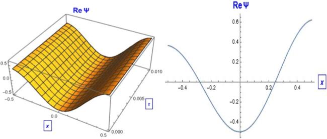
Figure 1. The 2D and 3D soliton solution behavior of equation ( |
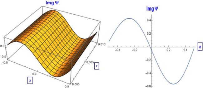
Figure 2. The 2D and 3D soliton solution behavior of equation ( |
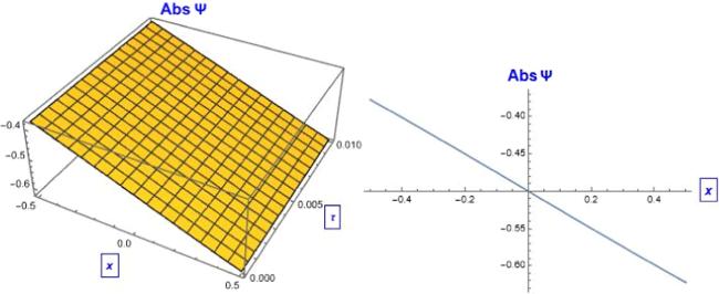
Figure 3. The 2D and 3D soliton solution behavior of $\left|{\rm{\Psi }}\right|$. |
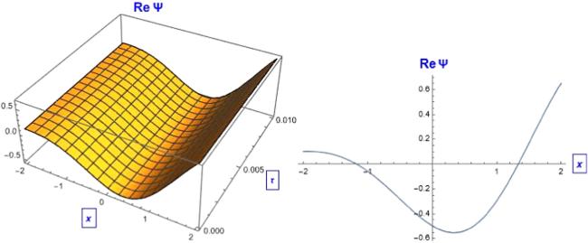
Figure 4. The 2D and 3D soliton solution behavior of equation ( |
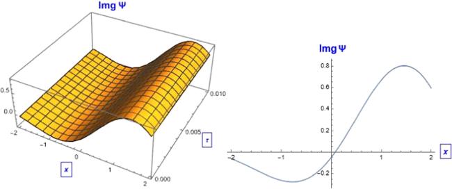
Figure 5. The 2D and 3D soliton solution behavior of equation ( |
By differentiating the first part of equation (1 ) with respect to the time we get
$\begin{eqnarray}\begin{array}{rcl}{\rm{i}}\hslash {{\rm{\Psi }}}_{\tau \tau } & = & \displaystyle \frac{-{\hslash }^{2}}{2m}{{\rm{\Psi }}}_{xx\tau }+{g}_{R}{n}_{R}{{\rm{\Psi }}}_{\tau }+{g}_{R}{\rm{\Psi }}{\left({n}_{R}\right)}_{\tau }\\ & & +\,\displaystyle \frac{{\rm{i}}\hslash }{2}\left(R{n}_{R}-{\gamma }_{c}\right){{\rm{\Psi }}}_{\tau }+\displaystyle \frac{{\rm{i}}\hslash R}{2}{\left({n}_{R}\right)}_{\tau }{\rm{\Psi }}\\ & & +\,{g}_{c}{\left({\left|{\rm{\Psi }}\right|}^{2}\right)}_{\tau }{\rm{\Psi }}+{g}_{c}{\left|{\rm{\Psi }}\right|}^{2}{\left({\rm{\Psi }}\right)}_{\tau }.\end{array}\end{eqnarray}$
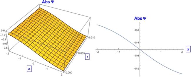
Figure 6. The 2D and 3D soliton solution behavior of $\left|{\rm{\Psi }}\right|$. |
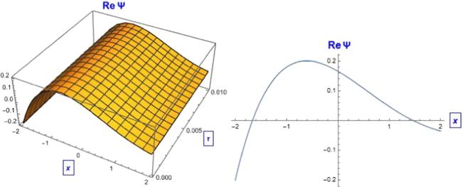
Figure 7. The soliton solution behaviors of equation ( |
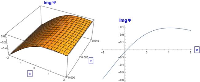
Figure 8. The soliton behavior of equation ( |
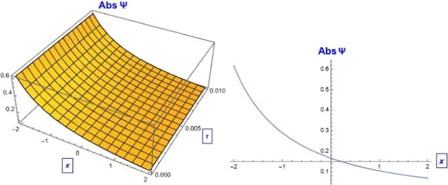
Figure 9. The 2D and 3D soliton solution behavior of $\left|{\rm{\Psi }}\right|$. |
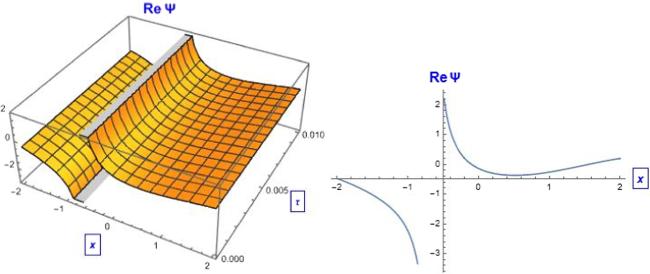
Figure 10. The soliton behavior of the Real (Re.) part of equation ( |
When the second part of equation (1 ) is substituted into equation (2 ) we get
$\begin{eqnarray}\begin{array}{c}\displaystyle \frac{{\hslash }^{2}}{2m}{{\rm{\Psi }}}_{xx\tau }+{\rm{i}}\hslash {{\rm{\Psi }}}_{\tau \tau }-{g}_{R}{n}_{R}{{\rm{\Psi }}}_{\tau }\\ \,-\,{g}_{R}{\rm{\Psi }}\left(P-{n}_{R}{\gamma }_{R}-{n}_{R}R{\left|{\rm{\Psi }}\right|}^{2}\right)\\ \,-\,\displaystyle \frac{{\rm{i}}\hslash }{2}\left(R{n}_{R}-{\gamma }_{c}\right){{\rm{\Psi }}}_{\tau }\\ \,-\,\displaystyle \frac{{\rm{i}}\hslash R}{2}\left(P-({\gamma }_{R}+R{\left|{\rm{\Psi }}\right|}^{2}){n}_{R}\right){\rm{\Psi }}\\ \,-\,{g}_{c}{\left({\left|{\rm{\Psi }}\right|}^{2}\right)}_{\tau }{\rm{\Psi }}-{g}_{c}{\left|{\rm{\Psi }}\right|}^{2}{{\rm{\Psi }}}_{\tau }=0.\end{array}\end{eqnarray}$
Let us now consider the complex transformation4 ), we can construct the following relations5 )–(10 ) are substituted into equation (3 ), which is dimensionless and $\hslash =m=1$, and the real and imaginary terms separated, we get
$\begin{eqnarray}\begin{array}{rcl}{\rm{\Psi }}\left(x,\tau \right) & = & u\left(\zeta \right){{\rm{e}}}^{i\eta (x,\tau )},\\ \zeta & = & k\,x+w\,\tau ,\\ \eta & = & qx+\delta \tau +{\vartheta }_{0},\end{array}\end{eqnarray}$
where $u\left(\eta \right)$ is the wave amplitude, while $\eta $ denotes the phase amplitude, where $k,{\vartheta }_{0},w$ are, respectively, frequency, phase constant and wave number. Simply from equation ( $\begin{eqnarray}{{\rm{\Psi }}}_{x}=\left(ku^{\prime} +{\rm{i}}\,qu\right){{\rm{e}}}^{{\rm{i}}\eta \left(x,\tau \right)},\end{eqnarray}$
$\begin{eqnarray}{{\rm{\Psi }}}_{xx}=\left(-{q}^{2}u+2{\rm{i}}kqu^{\prime} +{k}^{2}u^{\prime\prime} \right){{\rm{e}}}^{{\rm{i}}\eta \left(x,\tau \right)},\end{eqnarray}$
$\begin{eqnarray}\begin{array}{rcl}{{\rm{\Psi }}}_{xx\tau } & = & -w{q}^{2}u^{\prime} -{\rm{i}}\delta {q}^{2}u+2{\rm{i}}kqwu^{\prime\prime} \\ & & -2\delta qku^{\prime} +{k}^{2}wu^{\prime\prime\prime} +{\rm{i}}\delta {k}^{2}u^{\prime\prime} {{\rm{e}}}^{{\rm{i}}\eta \left(x,\tau \right)},\end{array}\end{eqnarray}$
$\begin{eqnarray}{{\rm{\Psi }}}_{\tau }=\left(wu^{\prime} +{\rm{i}}\,\delta u\right){{\rm{e}}}^{{\rm{i}}\eta \left(x,\tau \right)},\end{eqnarray}$
$\begin{eqnarray}{{\rm{\Psi }}}_{\tau \tau }=\left(-{\delta }^{2}u+2{\rm{i}}\delta wu^{\prime} +{w}^{2}u^{\prime\prime} \right){{\rm{e}}}^{{\rm{i}}\eta \left(x,\tau \right)},\end{eqnarray}$
$\begin{eqnarray}{\left|{\rm{\Psi }}\right|}^{2}={u}^{2}.\end{eqnarray}$
When the relations ( $\begin{eqnarray}\begin{array}{l}\displaystyle \frac{{k}^{2}w}{2}u^{\prime\prime\prime} -\left(\displaystyle \frac{1}{2}\left[w{q}^{2}+2\delta qk\right]+2\delta w+{g}_{R}{n}_{R}w\right)u^{\prime} \\ \,+\,\left({g}_{R}\left({\gamma }_{R}{n}_{R}-P\right)-\displaystyle \frac{\delta }{2}\left({\gamma }_{c}-R{n}_{R}\right)\right)u\\ \,-\,3{g}_{c}w{u}^{2}u^{\prime} +R{g}_{R}{n}_{R}{u}^{3}=0,\end{array}\end{eqnarray}$
$\begin{eqnarray}\begin{array}{c}\left(\displaystyle \frac{{k}^{2}\delta }{2}+kqw+{w}^{2}\right)u^{\prime\prime} +\left(\displaystyle \frac{{R}^{2}{n}_{R}}{2}-\delta {g}_{c}\right){u}^{3}\\ \,+\,\left(\displaystyle \frac{{\gamma }_{c}w}{2}-\displaystyle \frac{R{n}_{R}w}{2}\right)u^{\prime} \\ \,-\,\left(\displaystyle \frac{{q}^{2}\delta }{2}+{\delta }^{2}+{g}_{R}{n}_{R}\delta -\displaystyle \frac{R{\gamma }_{R}{n}_{R}}{2}+\displaystyle \frac{Rp}{2}\right)u=0.\end{array}\end{eqnarray}$
2. The GKT-concept
To discuss the Generalized Kudryashov Technique (GKT) concept, we will investigate the formalism of the nonlinear partial differential equation (NLPDE) by supposing the function $E$ of $u\left(x,\tau \right)$ and its partial derivatives as13 ), it will be replaced by the following ordinary differential equation14 ) according to the GKM is16 ) we get
$\begin{eqnarray}E\left(u,{u}_{x},{u}_{\tau },{u}_{xx},{u}_{\tau \tau },\ldots \right)=0.\end{eqnarray}$
When we apply the transformation $u\left(x,\tau \right)=u\left(\zeta \right),\zeta =kx+w\tau ,$ where $k,\omega $ are, respectively, the wave number and traveling wave speed to equation ( $\begin{eqnarray}R\left(u^{\prime} ,u^{\prime\prime} ,u^{\prime\prime\prime} ,\ldots \right)=0,\end{eqnarray}$
in which $R$ is a function of $u\left(x,\tau \right)$ and its total derivatives. The proposed solution of equation ( $\begin{eqnarray}u\left(\zeta \right)=\displaystyle \frac{\displaystyle {\sum }_{i=0}^{N}{a}_{i}{P}^{i}\left(\zeta \right)}{\displaystyle {\sum }_{j=0}^{M}{b}_{j}{P}^{j}\left(\zeta \right)}=\displaystyle \frac{{a}_{0}+{a}_{1}P\left(\zeta \right)+{a}_{2}{P}^{2}\left(\zeta \right)+\ldots }{{b}_{0}+{b}_{1}P(\zeta )+{b}_{2}{P}^{2}(\zeta )+\ldots },\end{eqnarray}$
where the parameters ${a}_{i},\left(i=0,1,2,\,\ldots ,\,N\right)$ and ${b}_{j},j\,=0,1,2,\,\ldots ,\,M$ will be determined later such that ${a}_{N}\ne 0,{b}_{M}\ne 0$, while the function $P\left(\zeta \right)$ is the solution of the second-order nonlinear equation. The solution for the real part with balance number M = 1 is $\begin{eqnarray}\displaystyle \frac{{\rm{d}}P\left(\zeta \right)}{{\rm{d}}\zeta }={P}^{2}\left(\zeta \right)-P\left(\zeta \right).\end{eqnarray}$
By integrating equation ( $\begin{eqnarray}P\left(\zeta \right)=\displaystyle \frac{1}{1+C{{\rm{e}}}^{\zeta }}.\end{eqnarray}$
Here, C is the integration constant. We will implement this method to the real part and the imaginary part individually.2.1. For the real part
When one applies the balance rule between $u^{\prime\prime\prime} ,{u}^{2}u^{\prime} $ appears at equation (11 ) he will obtain $M=1,\Rightarrow N=2$; thus, the solution is
$\begin{eqnarray}u\left(\zeta \right)=\displaystyle \frac{{a}_{0}+{a}_{1}P\left(\zeta \right)+{a}_{2}{P}^{2}\left(\zeta \right)}{{b}_{0}+{b}_{1}P\left(\zeta \right)}.\end{eqnarray}$
By inserting $u^{\prime\prime\prime} ,{u}^{2}u^{\prime} ,u,{u}^{3}$ into equation (11 ), setting the coefficients of various powers of ${P}^{i}(\zeta )$ equal to zero, a system of equations for the required unknown parameters will be explored from which we get 24 diverse enormous results; for similarity and simplicity, we will choose one of these results, which is
$\begin{eqnarray}\begin{array}{c}w\,\to \,-\displaystyle \frac{R{g}_{R}{n}_{R}}{3{g}_{c}},{a}_{0}\to 0,{b}_{0}\to 0,\\ {\gamma }_{c}\,\to \,\displaystyle \frac{-2P{g}_{c}{g}_{R}+R\delta {g}_{c}{n}_{R}+2{k}^{2}R{g}_{R}{n}_{R}+2{g}_{c}{g}_{R}{n}_{R}{\gamma }_{R}}{\delta {g}_{c}},\\ q\,\to \,\displaystyle \frac{3k\delta {g}_{c}+\sqrt{9{k}^{2}{\delta }^{2}{g}_{c}^{2}+7{k}^{2}{R}^{2}{g}_{R}^{2}{n}_{R}^{2}-4{R}^{2}\delta {g}_{R}^{2}{n}_{R}^{2}-2{R}^{2}{g}_{R}^{3}{n}_{R}^{3}}}{R{g}_{R}{n}_{R}},\\ {a}_{1}\,\to \,-{a}_{2},{b}_{1}\to \displaystyle \frac{{a}_{2}\sqrt{{g}_{c}}}{k}.\end{array}\end{eqnarray}$
Let us now design the 2D and 3D graphs of this solution that can be simplified to
$\begin{eqnarray}\begin{array}{c}C=\delta =R={g}_{c}={g}_{R}={\gamma }_{R}={n}_{R}=k=P={a}_{2}=1,\\ {a}_{0}=0,{a}_{1}=-1,{b}_{0}=0,{b}_{1}=1,\\ w=-0.3,{\gamma }_{c}=3,q=3+\sqrt{10}.\end{array}\end{eqnarray}$
The solution according to these parameter values is
$\begin{eqnarray}u\left(\zeta \right)=\displaystyle \frac{-{{\rm{e}}}^{\zeta }}{{{\rm{e}}}^{\zeta }+1},\end{eqnarray}$
$\begin{eqnarray}{\rm{\Psi }}\left(x,\tau \right)=\left(\displaystyle \frac{-{{\rm{e}}}^{\left(x-\tfrac{1}{3}\tau \right)}}{{{\rm{e}}}^{\left(x-\tfrac{1}{3}\tau \right)}+1}\right){{\rm{e}}}^{{\rm{i}}\left(6x+\tau +0.1\right)},\end{eqnarray}$
$\begin{eqnarray}\mathrm{Re}{\rm{\Psi }}\left(x,\tau \right)=\left(\displaystyle \frac{-{{\rm{e}}}^{\left(x-\tfrac{1}{3}\tau \right)}}{{{\rm{e}}}^{\left(x-\tfrac{1}{3}\tau \right)}+1}\right)\cos \left(6x+\tau +0.1\right),\end{eqnarray}$
$\begin{eqnarray}\rm{Im}{\rm{\Psi }}\left(x,\tau \right)=\left(\displaystyle \frac{-{{\rm{e}}}^{\left(x-\displaystyle \frac{1}{3}\tau \right)}}{{{\rm{e}}}^{\left(x-\displaystyle \frac{1}{3}\tau \right)}+1}\right)\sin \left(6x+\tau +0.1\right).\end{eqnarray}$
2.2. For the imaginary part
When one applies the balance rule between $u^{\prime\prime} ,{u}^{3}$ appears at equation (12 ) he will obtain $M=1;$ thus, the solution is
$\begin{eqnarray}u\left(\zeta \right)=\displaystyle \frac{{a}_{0}+{a}_{1}P\left(\zeta \right)+{a}_{2}{P}^{2}\left(\zeta \right)}{{b}_{0}+{b}_{1}P\left(\zeta \right)}.\end{eqnarray}$
By inserting $u^{\prime\prime} ,{u}^{3},u^{\prime} ,u$ into equation (12 ), setting the coefficients of various powers of ${P}^{i}\left(\zeta \right)$ equal to zero, a system of equations for the required unknown parameters will be explored, from which we get 14 diverse enormous results; for similarity and simplicity, we will choose one of them, which is
$\begin{eqnarray}\begin{array}{c}{a}_{0}\to 0,{b}_{0}\to 0,{\gamma }_{c}\to \displaystyle \frac{-6\delta {a}_{2}^{2}{g}_{c}+3{R}^{2}{a}_{2}^{2}{n}_{R}+2Rw{b}_{1}^{2}{n}_{R}}{2w{b}_{1}^{2}},\\ q\to \displaystyle \frac{-4{w}^{2}{b}_{1}^{2}-2{k}^{2}\delta {b}_{1}^{2}+2\delta {a}_{2}^{2}{g}_{c}-{R}^{2}{a}_{2}^{2}{n}_{R}}{4kw{b}_{1}^{2}},\\ P\to \displaystyle \frac{\left\{\begin{array}{c}-16{w}^{4}\delta {b}_{1}^{4}-48{k}^{2}{w}^{2}{\delta }^{2}{b}_{1}^{4}-4{k}^{4}{\delta }^{3}{b}_{1}^{4}-32{k}^{2}{w}^{2}\delta {a}_{2}^{2}{b}_{1}^{2}{g}_{c}+16{w}^{2}{\delta }^{2}{a}_{2}^{2}{b}_{1}^{2}{g}_{c}\\ +8{k}^{2}{\delta }^{3}{a}_{2}^{2}{b}_{1}^{2}{g}_{c}-4{\delta }^{3}{a}_{2}^{4}{g}_{c}^{2}+16{k}^{2}{R}^{2}{w}^{2}{a}_{2}^{2}{b}_{1}^{2}{n}_{R}-8{R}^{2}{w}^{2}\delta {a}_{2}^{2}{b}_{1}^{2}{n}_{R}-4{k}^{2}{R}^{2}{\delta }^{2}{a}_{2}^{2}{b}_{1}^{2}{n}_{R}\\ +4{R}^{2}{\delta }^{2}{a}_{2}^{4}{g}_{c}{n}_{R}-32{k}^{2}{w}^{2}\delta {b}_{1}^{4}{g}_{R}{n}_{R}-{R}^{4}\delta {a}_{2}^{4}{n}_{R}^{2}+16{k}^{2}R{w}^{2}{b}_{1}^{4}{n}_{R}{\gamma }_{R}\end{array}\right\}}{16{k}^{2}R{w}^{2}{b}_{1}^{4}},\\ {a}_{1}\to -{a}_{2}.\end{array}\end{eqnarray}$
Let us now design the 2D and 3D graphs of the chosen result that can be simplified to
$\begin{eqnarray}\begin{array}{c}\delta =R=w={n}_{R}={g}_{c}={a}_{2}={b}_{1}={\gamma }_{R}=k={g}_{R}=1,\\ {a}_{0}={b}_{0}=0,{a}_{1}=-1,{\gamma }_{c}=-\displaystyle \frac{1}{2},P=-\displaystyle \frac{89}{16},q=-\displaystyle \frac{5}{4}.\end{array}\end{eqnarray}$
The solution according to these parameter values is
$\begin{eqnarray}u\left(\zeta \right)=\displaystyle \frac{-{{\rm{e}}}^{\zeta }}{{{\rm{e}}}^{\zeta }+1},\end{eqnarray}$
$\begin{eqnarray}{\rm{\Psi }}\left(x,\tau \right)=\left(\displaystyle \frac{-{{\rm{e}}}^{\left(x+\tau \right)}}{{{\rm{e}}}^{x+\tau }+1}\right){{\rm{e}}}^{{\rm{i}}\left(\tfrac{-5}{4}x+\tau +0.1\right)},\end{eqnarray}$
$\begin{eqnarray}\mathrm{Re}{\rm{\Psi }}\left(x,\tau \right)=\left(\displaystyle \frac{-{{\rm{e}}}^{\left(x+\tau \right)}}{{{\rm{e}}}^{\left(x+\tau \right)}+1}\right)\cos \left(\displaystyle \frac{-5}{4}x+\tau +0.1\right),\end{eqnarray}$
$\begin{eqnarray}\rm{Im}{\rm{\Psi }}\left(x,\tau \right)=\left(\displaystyle \frac{-{{\rm{e}}}^{\left(x+\tau \right)}}{{{\rm{e}}}^{\left(x+\tau \right)}+1}\right)\sin \left(\displaystyle \frac{-5}{4}x+\tau +0.1\right).\end{eqnarray}$
3. The (G′/G)-expansion scheme
This scheme proposes the solution of equation (14 ) to be in the form
$\begin{eqnarray}u\left(\eta \right)={A}_{0}+{\displaystyle \sum _{i=1}^{M}{A}_{i}\left[\displaystyle \frac{G^{\prime} }{G}\right]}^{i},{A}_{M}\ne 0,\end{eqnarray}$
where $M$ is the balance number. The function $G\left(\zeta \right)$ achieves the second-order differential equation $G^{\prime\prime} +\mu G^{\prime} +\lambda G=0$ that has three types of solution depending on the discriminate of this equation, which has one of these cases:(I) If ${\mu }^{2}-4\lambda \succ 0,$ then the solution is
$\begin{eqnarray}\begin{array}{c}\left(\displaystyle \frac{G^{\prime} }{G}\right)\,=\displaystyle \frac{\sqrt{{\mu }^{2}-4\lambda }}{2}\\ \times \,\left(\displaystyle \frac{{l}_{1}\,\sinh \left(\displaystyle \frac{\sqrt{{\mu }^{2}-4\lambda }}{2}\right)\zeta +{l}_{2}\,\cosh \left(\displaystyle \frac{\sqrt{{\mu }^{2}-4\lambda }}{2}\right)\zeta }{{l}_{1}\,\cosh \left(\displaystyle \frac{\sqrt{{\mu }^{2}-4\lambda }}{2}\right)\zeta +{l}_{2}\,\sinh \left(\displaystyle \frac{\sqrt{{\mu }^{2}-4\lambda }}{2}\right)\zeta }\right)\\ \,-\,\displaystyle \frac{\mu }{2}.\end{array}\end{eqnarray}$
(II) If ${\mu }^{2}-4\lambda \prec 0\,{,}\,$ then the solution is
$\begin{eqnarray}\begin{array}{c}\left(\displaystyle \frac{G^{\prime} }{G}\right)=\,\displaystyle \frac{\sqrt{{\mu }^{2}-4\lambda }}{2}\\ \times \,\left(\displaystyle \frac{-{l}_{1}\,\sin \left(\displaystyle \frac{\sqrt{{\mu }^{2}-4\lambda }}{2}\right)\zeta +{l}_{2}\,\cos \left(\displaystyle \frac{\sqrt{{\mu }^{2}-4\lambda }}{2}\right)\zeta }{{l}_{1}\,\cos \left(\displaystyle \frac{\sqrt{{\mu }^{2}-4\lambda }}{2}\right)\zeta +{l}_{2}\,\sin \left(\displaystyle \frac{\sqrt{{\mu }^{2}-4\lambda }}{2}\right)\zeta }\right)\\ \,-\,\displaystyle \frac{\mu }{2}.\end{array}\end{eqnarray}$
(III) If ${\mu }^{2}-4\lambda =0\,{,}\,$ then the solution is
$\begin{eqnarray}\left(\displaystyle \frac{G^{\prime} }{G}\right)=\left(\displaystyle \frac{{l}_{2}}{{l}_{1}+{l}_{2}\zeta }\right)-\displaystyle \frac{\mu }{2}.\end{eqnarray}$
Let us now apply this concept for the above real part and imaginary part of equations (11 ) and (12 ), respectively.
3.1. Solution for the real part with balance number $M=1$
$\begin{eqnarray}u(\zeta )={A}_{0}+{A}_{1}\left(\displaystyle \frac{G^{\prime} }{G}\right).\end{eqnarray}$
By computing $u^{\prime\prime\prime} ,{u}^{2}u^{\prime} ,u,{u}^{3}$ and inserting in equation (11 ), setting the coefficients of various powers of ${\left(\displaystyle \frac{G^{\prime} }{G}\right)}^{i}$ equal to zero, a system of equations for the required unknown parameters will be explored, from which we get unique result, which is
$\begin{eqnarray}\begin{array}{c}\lambda \to \displaystyle \frac{{A}_{0}\left(3{k}^{2}w{A}_{0}+R{A}_{1}^{3}{g}_{R}{n}_{R}\right)}{3{k}^{2}w{A}_{1}^{2}},\\ \mu \to \displaystyle \frac{6{k}^{2}w{A}_{0}+R{A}_{1}^{3}{g}_{R}{n}_{R}}{3{k}^{2}w{A}_{1}},\\ \delta \to \displaystyle \frac{-9{k}^{2}{q}^{2}{w}^{2}-18{k}^{2}{w}^{2}{g}_{R}{n}_{R}+7{R}^{2}{A}_{1}^{4}{g}_{R}^{2}{n}_{R}^{2}}{18{k}^{2}w\left(kq+2w\right)},\\ {\gamma }_{c}\to \left(\displaystyle \frac{\begin{array}{c}36{k}^{5}Pq{w}^{2}{g}_{R}+72{k}^{4}P{w}^{3}{g}_{R}+9{k}^{4}{q}^{2}R{w}^{3}{n}_{R}+18{k}^{4}R{w}^{3}{g}_{R}{n}_{R}^{2}-7{k}^{2}{R}^{3}w{A}_{1}^{4}{g}_{R}^{2}{n}_{R}^{3}\\ -4kq{R}^{3}{A}_{1}^{6}{g}_{R}^{3}{n}_{R}^{3}-8{R}^{3}w{A}_{1}^{6}{g}_{R}^{3}{n}_{R}^{3}-36{k}^{5}q{w}^{2}{g}_{R}{n}_{R}{\gamma }_{R}-72{k}^{4}{w}^{3}{g}_{R}{n}_{R}\gamma \end{array}}{{k}^{2}w\left(9{k}^{2}{q}^{2}{w}^{2}+18{k}^{2}{w}^{2}{g}_{R}{n}_{R}-7{R}^{2}{A}_{1}^{4}{g}_{R}^{2}{n}_{R}^{2}\right)}\right),\\ {g}_{c}\to \displaystyle \frac{{k}^{2}}{{A}_{1}^{2}}.\end{array}\end{eqnarray}$
This result can be streamlined to the following values11 ) for $\left(\displaystyle \frac{G^{\prime} }{G}\right)$ cases is
$\begin{eqnarray}\begin{array}{l}{g}_{R}=k=R={A}_{1}=w={\gamma }_{R}\\ \,=\,{A}_{0}=P=q={n}_{R}={g}_{c}=1,\\ \lambda =\displaystyle \frac{4}{3},\mu =\displaystyle \frac{7}{3},{\gamma }_{c}=\displaystyle \frac{2}{5},\delta \to -\displaystyle \frac{10}{27},\end{array}\end{eqnarray}$
from which we have ${\mu }^{2}-4\lambda =\displaystyle \frac{1}{9}\succ 0,$ which implies the form equation ( $\begin{eqnarray}\left(\displaystyle \frac{G^{\prime} }{G}\right)=\displaystyle \frac{1}{6}\left(\displaystyle \frac{{l}_{1}\,{\rm{\sin }}\,{\rm{h}}\left(\tfrac{1}{6}\right)\zeta +{l}_{2}\,{\rm{\cos }}\,{\rm{h}}\left(\tfrac{1}{6}\right)\zeta }{{l}_{1}\,{\rm{\cos }}\,{\rm{h}}\left(\tfrac{1}{6}\right)\zeta +{l}_{2}\,{\rm{\sin }}\,{\rm{h}}\left(\tfrac{1}{6}\right)\zeta }\right)-\displaystyle \frac{7}{6},\end{eqnarray}$
$\begin{eqnarray}\begin{array}{rcl}u\left(\zeta \right) & = & 1+\displaystyle \frac{1}{6}\left(\displaystyle \frac{{l}_{1}\,{\rm{\sin }}\,{\rm{h}}\left(\tfrac{1}{6}\right)\zeta +{l}_{2}\,{\rm{\cos }}\,{\rm{h}}\left(\tfrac{1}{6}\right)\zeta }{{l}_{1}\,{\rm{\cos }}\,{\rm{h}}\left(\tfrac{1}{6}\right)\zeta +{l}_{2}\,{\rm{\sin }}\,{\rm{h}}\left(\tfrac{1}{6}\right)\zeta }\right)-\displaystyle \frac{7}{6}\\ & = & \displaystyle \frac{1}{6}\left(\displaystyle \frac{{l}_{1}\,{\rm{\sin }}\,{\rm{h}}\left(\tfrac{1}{6}\right)\zeta +{l}_{2}\,{\rm{\cos }}\,{\rm{h}}\left(\tfrac{1}{6}\right)\zeta }{{l}_{1}\,\cosh \left(\tfrac{1}{6}\right)\zeta +{l}_{2}\,\sinh \left(\tfrac{1}{6}\right)\zeta }-1\right),\end{array}\end{eqnarray}$
$\begin{eqnarray}\begin{array}{l}{\rm{\Psi }}\left(x,\tau \right)\,=\displaystyle \frac{1}{6}\\ \times \,\left(\displaystyle \frac{{l}_{1}\,{\rm{\sin }}\,{\rm{h}}\left(\tfrac{1}{6}\left(x+\tau \right)\right)+{l}_{2}\,{\rm{\cos }}\,{\rm{h}}\left(\tfrac{1}{6}\left(x+\tau \right)\right)}{{l}_{1}\,{\rm{\cos }}\,{\rm{h}}\left(\tfrac{1}{6}\left(x+\tau \right)\right)+{l}_{2}\,{\rm{\sin }}\,{\rm{h}}\left(\tfrac{1}{6}\left(x+\tau \right)\right)}-1\right)\\ \times \,{{\rm{e}}}^{{\rm{i}}\left(x-\,\tfrac{10}{27}\tau +0.1\right)},\end{array}\end{eqnarray}$
$\begin{eqnarray}\begin{array}{l}\mathrm{Re}{\rm{\Psi }}\left(x,\tau \right)\,=\displaystyle \frac{1}{6}\\ \times \,\left(\displaystyle \frac{{l}_{1}\,{\rm{\sin }}\,{\rm{h}}\left(\tfrac{1}{6}\left(x+\tau \right)\right)+{l}_{2}\,{\rm{\cos }}\,{\rm{h}}\left(\tfrac{1}{6}\left(x+\tau \right)\right)}{{l}_{1}\,{\rm{\cos }}\,{\rm{h}}\left(\tfrac{1}{6}\left(x+\tau \right)\right)+{l}_{2}\,{\rm{\sin }}\,{\rm{h}}\left(\tfrac{1}{6}\left(x+\tau \right)\right)}-1\right)\\ \times \,\cos \left(x-\displaystyle \frac{10}{27}\tau +0.1\right),\end{array}\end{eqnarray}$
$\begin{eqnarray}\begin{array}{l}\rm{Im}{\rm{\Psi }}\left(x,\tau \right)\,=\displaystyle \frac{1}{6}\\ \times \,\left(\displaystyle \frac{{l}_{1}\,{\rm{\sin }}\,{\rm{h}}\left(\displaystyle \frac{1}{6}\left(x+\tau \right)\right)+{l}_{2}\,\cos \,{\rm{h}}\left(\displaystyle \frac{1}{6}\left(x+\tau \right)\right)}{{l}_{1}\,\cos \,{\rm{h}}\left(\displaystyle \frac{1}{6}\left(x+\tau \right)\right)+{l}_{2}\,{\rm{\sin }}\,{\rm{h}}\left(\displaystyle \frac{1}{6}\left(x+\tau \right)\right)}-1\right)\\ \times \,\sin \left(x-\displaystyle \frac{10}{27}\tau +0.1\right).\end{array}\end{eqnarray}$
Let us now design the 2D and 3D graphs of equations (42 ) and (43 )
3.2. The (G′/G)-expansion scheme for the imaginary part
As we noted before, the balance number for imaginary part equation (12 ) is $M=1;$ hence, the solution is
$\begin{eqnarray}u\left(\zeta \right)={A}_{0}+{A}_{1}\left(\displaystyle \frac{G^{\prime} }{G}\right).\end{eqnarray}$
By computing $u^{\prime\prime} ,u^{\prime} ,u,{u}^{3}$ and inserting in equation (12 ), setting the coefficients of various powers of ${\left(\displaystyle \frac{G^{\prime} }{G}\right)}^{i}$ equal to zero, a system of equations for the required unknown parameters will be explored, from which we get three different results; for simplicity we choose the first one, which is
$\begin{eqnarray}\begin{array}{c}\lambda \to \displaystyle \frac{4kqw{A}_{0}^{2}+4{w}^{2}{A}_{0}^{2}+2{k}^{2}\delta {A}_{0}^{2}+PR{A}_{1}^{2}+{q}^{2}\delta {A}_{1}^{2}+2{\delta }^{2}{A}_{1}^{2}+2\delta {A}_{1}^{2}{g}_{R}{n}_{R}-R{A}_{1}^{2}{n}_{R}{\gamma }_{R}}{2\left(2kqw+2{w}^{2}+{k}^{2}\delta \right){A}_{1}^{2}},\\ \mu \to \displaystyle \frac{2{A}_{0}}{{A}_{1}},{g}_{c}\to \displaystyle \frac{4kqw+4{w}^{2}+2{k}^{2}\delta +{R}^{2}{A}_{1}^{2}{n}_{R}}{2\delta {A}_{1}^{2}},{\gamma }_{c}\to R{n}_{R}.\end{array}\end{eqnarray}$
This result can be streamlined to be in the form12 ) is
$\begin{eqnarray}\begin{array}{l}{g}_{R}=k=R={A}_{1}=w={\gamma }_{R}\\ \,=\,{A}_{0}=P=q=\delta ={n}_{R}={\gamma }_{c}=1,\\ \lambda =\displaystyle \frac{3}{2},\mu =2,{g}_{c}=\displaystyle \frac{11}{2},\end{array}\end{eqnarray}$
from which we have ${\mu }^{2}-4\lambda =-2\prec 0,$ so the solution from $\left(\displaystyle \frac{G^{\prime} }{G}\right)$ point of view equation ( $\begin{eqnarray}u\left(\zeta \right)=\displaystyle \frac{{\rm{i}}}{\sqrt{2}}\left(\displaystyle \frac{-{l}_{1}\,\sin \left(\tfrac{{\rm{i}}}{\sqrt{2}}\right)\zeta +{l}_{2}\,\cos \left(\tfrac{{\rm{i}}}{\sqrt{2}}\right)\zeta }{{l}_{1}\,\cos \left(\tfrac{{\rm{i}}}{\sqrt{2}}\right)\zeta +{l}_{2}\,\sin \left(\tfrac{{\rm{i}}}{\sqrt{2}}\right)\zeta }\right),\end{eqnarray}$
$\begin{eqnarray}\begin{array}{l}{\rm{\Psi }}\left(x,\tau \right)\,=\displaystyle \frac{{\rm{i}}}{\sqrt{2}}\\ \times \,\left(\displaystyle \frac{-{l}_{1}\,\sin \left(\tfrac{{\rm{i}}\left(x+\tau \right)}{\sqrt{2}}\right)+{l}_{2}\,\cos \left(\tfrac{{\rm{i}}\left(x+\tau \right)}{\sqrt{2}}\right)}{{l}_{1}\,\cos \left(\tfrac{{\rm{i}}\left(x+\tau \right)}{\sqrt{2}}\right)+{l}_{2}\,\sin \left(\tfrac{{\rm{i}}\left(x+\tau \right)}{\sqrt{2}}\right)}\right)\\ \times \,{{\rm{e}}}^{{\rm{i}}\left(x+\tau +0.1\right)},\end{array}\end{eqnarray}$
$\begin{eqnarray}\begin{array}{l}\mathrm{Re}{\rm{\Psi }}\left(x,\tau \right)\,=\displaystyle \frac{-{\rm{i}}}{\sqrt{2}}\\ \times \,\left(\displaystyle \frac{-{l}_{1}\,\sin \left(\tfrac{{\rm{i}}\left(x+\tau \right)}{\sqrt{2}}\right)+{l}_{2}\,\cos \left(\tfrac{{\rm{i}}\left(x+\tau \right)}{\sqrt{2}}\right)}{{l}_{1}\,\cos \left(\tfrac{{\rm{i}}\left(x+\tau \right)}{\sqrt{2}}\right)+{l}_{2}\,\sin \left(\tfrac{{\rm{i}}\left(x+\tau \right)}{\sqrt{2}}\right)}\right)\\ \times \,\sin \left(x+\tau +0.1\right),\end{array}\end{eqnarray}$
$\begin{eqnarray}\begin{array}{c}\rm{Im}{\rm{\Psi }}\left(x,\tau \right)\,=\displaystyle \frac{{\rm{i}}}{\sqrt{2}}\\ \times \,\left(\displaystyle \frac{-{l}_{1}\,\sin \left(\displaystyle \frac{{\rm{i}}\left(x+\tau \right)}{\sqrt{2}}\right)+{l}_{2}\,\cos \left(\displaystyle \frac{{\rm{i}}\left(x+\tau \right)}{\sqrt{2}}\right)}{{l}_{1}\,\cos \left(\displaystyle \frac{{\rm{i}}\left(x+\tau \right)}{\sqrt{2}}\right)+{l}_{2}\,\sin \left(\displaystyle \frac{{\rm{i}}\left(x+\tau \right)}{\sqrt{2}}\right)}\right)\\ \times \,\cos \left(x+\tau +0.1\right).\end{array}\end{eqnarray}$
4. The algorithm of HWNS
The wavelet is considered as one of the powerful and fast evolving methods to obtain a numerical solution of ordinary and partial differential equations with increasing applications in physics and engineering problems. The development of the Haar wavelet in the construction of the numerical solution started in 1997 when Chen and Hsiao [41] introduced an operational matrix of integration to solve the suggested models of dynamic systems. They suggested the notation of expressing the function corresponding to highest derivative of a differential equation as a Haar wavelet series. Lepik [42–44] introduced the Haar wavelet numerical scheme with a uniform grid for the solution of differential, integral, integro-differential and fractional integral equations. As a vital part of this work, we attempt to extend this method to examine the results for higher order nonlinear boundary value problems with semi-infinite or infinite domain, thus making the method more useful in real-world applications.
4.1. Haar wavelet functions and their integration
The Haar wavelet functions [45] are given as
$\begin{eqnarray}{h}_{i}\left(t\right)=\left\{\begin{array}{ll}1; & for\,t\in \left[{\nu }_{1},{\nu }_{2}\right]\\ -1; & for\,t\in \left[{\nu }_{2},{\nu }_{2}\right]\\ 0; & {\rm{otherwise}}\end{array}\right..\end{eqnarray}$
This is considered as the simplest wavelet function in the structure of building basis functions because it uses only two operations, translation and dilation.With ${\nu }_{1}=\displaystyle \frac{k}{m},$ ${\nu }_{2}=\displaystyle \frac{k+0.5}{m},$ ${\nu }_{3}=\tfrac{k+1}{m}:$ the integer number $m={2}^{j};\,j=0,1,2,\,\ldots ,\,J$ indicates the level of the wavelet (dilation parameter); and $k=0,1,2,\,\ldots ,\,m-1$ is the translation parameter. The integer $J$ is the maximal level of resolution; the index $i$ is computed from $i=m+k+1$, which has minimum value $i=2\left(m=1,k=0\right),$ for which the Haar function is called the mother function, and maximum value $i=2M,$ $M={2}^{J}$ the index $i=1$ corresponds to the scaling (father) function:
$\begin{eqnarray}{h}_{1}\left(t\right)=\left\{\begin{array}{ll}1; & for\,0\leqslant t\prec 1\\ 0; & elsewhere\end{array}\right..\end{eqnarray}$
The following relations according to [41–45] are important to introduce
$\begin{eqnarray}\begin{array}{rcl}{p}_{i}\left(t\right) & = & {\int }_{0}^{t}{h}_{i}\left(x\right){\rm{d}}x;\\ {Q}_{i}\left(t\right) & = & {\int }_{0}^{t}{p}_{i}\left(x\right){\rm{d}}x;\\ {R}_{i}\left(t\right) & = & {\int }_{0}^{t}{Q}_{i}\left(x\right){\rm{d}}x.\end{array}\end{eqnarray}$
Integrating the Haar functions with respect to $t$ from $0\to x$, we can obtain the following important special relations:
$\begin{eqnarray}{p}_{i}\left(t\right)=\left\{\begin{array}{cc}t-{\nu }_{1}; & for\,t\in \left[{\nu }_{1},\,{\nu }_{2}\right]\\ {\nu }_{3}-t; & for\,t\in \left[{\nu }_{2},\,{\nu }_{3}\right]\\ 0; & elsewhere\end{array}\right.,\end{eqnarray}$
$\begin{eqnarray}{Q}_{i}\left(t\right)=\left\{\begin{array}{ll}0; & for\,t\in \left[0,{\nu }_{1}\right]\\ \frac{{\left(t-{\nu }_{1}\right)}^{2}}{2}; & for\,t\in \left[{\nu }_{1},{\nu }_{2}\right]\\ \frac{1}{4{m}^{2}}-\frac{{\left({\nu }_{3}-t\right)}^{2}}{2}; & for\,t\in \left[{\nu }_{2},{\nu }_{3}\right]\\ \frac{1}{4{m}^{2}}; & for\,t\in \left[{\nu }_{3},1\right]\end{array},\right.\end{eqnarray}$
$\begin{eqnarray}{R}_{i}\left(t\right)=\Space{0ex}{3.0ex}{0ex}\{\begin{array}{ll}0; & for\,t\in \left[0,{\nu }_{1}\right]\\ \displaystyle \frac{{\left(t-{\nu }_{1}\right)}^{3}}{6}; & for\,t\in \left[{\nu }_{1},{\nu }_{2}\right]\\ \displaystyle \frac{\left(t-{\nu }_{2}\right)}{4{m}^{2}}-\displaystyle \frac{{\left({\nu }_{3}-t\right)}^{3}}{6}; & for\,t\in \left[{\nu }_{2},{\nu }_{3}\right]\\ \displaystyle \frac{t-{\nu }_{2}}{4{m}^{2}}; & for\,t\in \left[{\nu }_{3},1\right]\end{array}.\end{eqnarray}$
Since the numerical solution is computed first at discrete points, in this case called collation points, to find the solution of the differential equation we discretize the equation in Haar functions ${h}_{i}\left(t\right)$ in the following manner.
Firstly, we will divide the interval $t\in \left[0,1\right]$ into 2M parts of equal length ${\rm{\Lambda }}\left(t\right)=\displaystyle \frac{1}{2M},$ then we compute the collocation points from
$\begin{eqnarray}{t}_{l}=\displaystyle \frac{l-0.5}{2M}.\end{eqnarray}$
Any function $\psi \left(t\right),t\in \left[0,1\right]$ can be written as58 ) by ${h}_{m}\left(t\right),$ and integrating from $0\to 1$, one obtains
$\begin{eqnarray}\psi \left(t\right)=\displaystyle \sum _{i=1}^{2M}{a}_{i}{h}_{i}\left(t\right)={a}_{1}{h}_{1}\left(t\right)+{a}_{2}{h}_{2}\left(t\right)+\,\ldots +{a}_{2M}{h}_{2M}\left(t\right),\end{eqnarray}$
where αi denotes the Haar coefficients. Multiplying equation ( $\begin{eqnarray*}\displaystyle {\int }_{0}^{1}\psi \left(t\right){h}_{m}\left(t\right){\rm{d}}t={a}_{i}\displaystyle \sum _{i=1}^{2M}\displaystyle {\int }_{0}^{1}{h}_{i}\left(t\right){h}_{m}\left(t\right){\rm{d}}t.\end{eqnarray*}$
And from the orthogonal property, we get the coefficients ${a}_{i}$ $\begin{eqnarray}\begin{array}{c}\displaystyle {\int }_{0}^{1}{h}_{i}\left(t\right){h}_{m}\left(t\right){\rm{d}}t=\left\{\begin{array}{ll}{2}^{-j}; & if\,i=m\\ 0; & if\,i\ne m\end{array}\right.\Rightarrow \\ \left[{a}_{i}={2}^{j}\displaystyle {\int }_{0}^{1}\psi \left(t\right){h}_{m}\left(t\right){\rm{d}}t\right].\end{array}\end{eqnarray}$
Satisfying equation (58 ) at collocation points
$\begin{eqnarray}\psi \left({t}_{l}\right)=\displaystyle \sum _{i=1}^{2M}{a}_{i}{h}_{i}\left({t}_{l}\right)=\displaystyle \sum _{i=1}^{2M}{a}_{i}{{\rm X}}_{il},\end{eqnarray}$
which can be written in matrix form ${\rm{\Xi }}=a{\rm X},$ where ${\rm{\Xi }}$ and $a$ are $2M$ vectors and ${\rm X}={{\rm X}}_{il}={h}_{i}\left({t}_{l}\right)$ are the coefficients matrix with dimension ($2M\times 2M).$4.3. The numerical solution using the HWNS corresponding to the exact solution derived by GKS (real part)
It is a vital aim in this work to construct the numerical solution corresponding to the analytical soliton solution obtained by GKS and the $\left(\displaystyle \frac{G^{\prime} }{G}\right)$-expansion scheme to show the reliability of the obtained analytical soliton solutions.
Consider the real part of equation (11 ) with values 21 ), which has the following initial conditions62 ) is put in the form64 ) three times w.r.t. $\zeta $ from $0\to \zeta $ to obtain $u\left(\zeta \right)$ we obtain64 )–(67 ) into equation (62 ) we obtain68 ) surrenders to the collocation points given in equation (57 ) we get69 ) becomes70 ), at collocation points ${\zeta }_{l}=\displaystyle \frac{l-0.5}{2M}\,=\displaystyle \frac{l-0.5}{4},l=1,2,3,4$, leads to a system of unknowns ${a}_{i},i=1,2,3,4,$ and by solving this system we get
$\begin{eqnarray}\begin{array}{c}\delta =R={g}_{c}={g}_{R}={\gamma }_{R}={n}_{R}=k=P=1,\\ w=\displaystyle \frac{-1}{3},{\gamma }_{c}=3,q=3+\sqrt{10}.\end{array}\end{eqnarray}$
This can be written as $\begin{eqnarray}\displaystyle \frac{1}{2}u^{\prime\prime\prime} \left(\zeta \right)+u^{\prime} \left(\zeta \right)+u^{\prime} \left(\zeta \right){u}^{2}\left(\zeta \right)-u\left(\zeta \right)+{u}^{3}\left(\zeta \right)=0,\end{eqnarray}$
whose exact solution derived by GKM is equation ( $\begin{eqnarray}u\left(0\right)=-\displaystyle \frac{1}{2},u^{\prime} \left(0\right)\,=-\displaystyle \frac{1}{4},u^{\prime\prime} \left(0\right)=0.\end{eqnarray}$
According to HWNS, the solution of equation ( $\begin{eqnarray}u^{\prime\prime\prime} \left(\zeta \right)=\displaystyle \sum _{i=1}^{2M}{a}_{i}{h}_{i}\left(\zeta \right).\end{eqnarray}$
By integrating equation ( $\begin{eqnarray}u^{\prime\prime} \left(\zeta \right)=\displaystyle \sum _{i=1}^{2M}{a}_{i}{p}_{i}\left(\zeta \right)+u^{\prime\prime} \left(0\right)=\displaystyle \sum _{i=1}^{2M}{a}_{i}{p}_{i}\left(\zeta \right),\end{eqnarray}$
$\begin{eqnarray}\displaystyle \begin{array}{rcl}u^{\prime} \left(\zeta \right) & = & \sum _{i=1}^{2M}{a}_{i}{Q}_{i}\left(\zeta \right)+u^{\prime} \left(0\right)\\ & = & -\displaystyle \frac{1}{4}+\sum _{i=1}^{2M}{a}_{i}{Q}_{i}\left(\zeta \right),\end{array}\end{eqnarray}$
$\begin{eqnarray}\displaystyle \begin{array}{rcl}u\left(\zeta \right) & = & \sum _{i=1}^{2M}{a}_{i}{R}_{i}\left(\zeta \right)-\frac{1}{4}\zeta +u\left(0\right)\\ & = & -\frac{1}{2}-\frac{1}{4}\zeta +\sum _{i=1}^{2M}{a}_{i}{R}_{i}\left(\zeta \right).\end{array}\end{eqnarray}$
Inserting equations ( $\begin{eqnarray}\begin{array}{c}\displaystyle \frac{1}{2}\displaystyle \sum _{i=1}^{2M}{a}_{i}{h}_{i}\left(\zeta \right)\,-\displaystyle \frac{1}{4}+\displaystyle \sum _{i=1}^{2M}{a}_{i}{Q}_{i}\left(\zeta \right)\\ \,+\,\left(-\displaystyle \frac{1}{4}+\displaystyle \sum _{i=1}^{2M}{a}_{i}{Q}_{i}\left(\zeta \right)\right){\left(-\displaystyle \frac{1}{2}-\displaystyle \frac{1}{4}\zeta +\displaystyle \sum _{i=1}^{2M}{a}_{i}{R}_{i}\left(\zeta \right)\right)}^{2}\\ \,+\,\displaystyle \frac{1}{2}+\displaystyle \frac{1}{4}\zeta -\displaystyle \sum _{i=1}^{2M}{a}_{i}{R}_{i}\left(\zeta \right)\\ \,+\,{\left(-\displaystyle \frac{1}{2}-\displaystyle \frac{1}{4}\zeta +\displaystyle \sum _{i=1}^{2M}{a}_{i}{R}_{i}\left(\zeta \right)\right)}^{3}=0.\end{array}\end{eqnarray}$
When equation ( $\begin{eqnarray}\begin{array}{c}\displaystyle \frac{1}{2}\displaystyle \sum _{i=1}^{2M}{a}_{i}{h}_{i}\left({\zeta }_{l}\right)-\displaystyle \frac{1}{4}+\displaystyle \sum _{i=1}^{2M}{a}_{i}{Q}_{i}\left({\zeta }_{l}\right)\\ \,+\,\left(-\displaystyle \frac{1}{4}+\displaystyle \sum _{i=1}^{2M}{a}_{i}{Q}_{i}\left(\zeta \right)\right){\left(-\displaystyle \frac{1}{2}-\displaystyle \frac{1}{4}{\zeta }_{l}+\displaystyle \sum _{i=1}^{2M}{a}_{i}{R}_{i}\left({\zeta }_{l}\right)\right)}^{2}\\ \,+\,\displaystyle \frac{1}{2}+\displaystyle \frac{1}{4}{\zeta }_{l}-\displaystyle \sum _{i=1}^{2M}{a}_{i}{R}_{i}\left({\zeta }_{l}\right)\\ \,+\,{\left(-\displaystyle \frac{1}{2}-\displaystyle \frac{1}{4}{\zeta }_{l}+\displaystyle \sum _{i=1}^{2M}{a}_{i}{R}_{i}\left({\zeta }_{l}\right)\right)}^{3}=0\,{,}\,l=1,2,\,\ldots ,\,2M.\end{array}\end{eqnarray}$
Putting the level of resolution $J=1\to M={2}^{J}\,=2\to 2M=4\to l=1,2,3,4$, then equation ( $\begin{eqnarray}\begin{array}{c}\displaystyle \frac{1}{2}\displaystyle \sum _{i=1}^{4}{a}_{i}{h}_{i}\left({\zeta }_{l}\right)-\displaystyle \frac{1}{4}+\displaystyle \sum _{i=1}^{4}{a}_{i}{Q}_{i}\left({\zeta }_{l}\right)\\ \,+\,\left(-\displaystyle \frac{1}{4}+\displaystyle \sum _{i=1}^{4}{a}_{i}{Q}_{i}\left(\zeta \right)\right){\left(-\displaystyle \frac{1}{2}-\displaystyle \frac{1}{4}{\zeta }_{l}+\displaystyle \sum _{i=1}^{4}{a}_{i}{R}_{i}\left({\zeta }_{l}\right)\right)}^{2}\\ \,+\,\displaystyle \frac{1}{2}+\displaystyle \frac{1}{4}{\zeta }_{l}-\displaystyle \sum _{i=1}^{4}{a}_{i}{R}_{i}\left({\zeta }_{l}\right)\\ \,+\,{\left(-\displaystyle \frac{1}{2}-\displaystyle \frac{1}{4}{\zeta }_{l}+\displaystyle \sum _{i=1}^{4}{a}_{i}{R}_{i}\left({\zeta }_{l}\right)\right)}^{3}=0\,.\end{array}\end{eqnarray}$
Equation ( $\begin{eqnarray}\begin{array}{rcl}{a}_{1} & = & -0.00279276,\\ {a}_{2} & = & -0.0929915,\\ {a}_{3} & = & -0.0262158,\\ {a}_{4} & = & -0.0656008.\end{array}\end{eqnarray}$
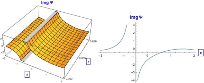
Figure 11. The soliton behavior of the Imaginary (Im.) part of equation ( |
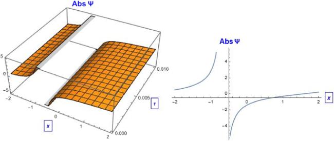
Figure 12. The 2D and 3D soliton solution behavior of $\left|{\rm{\Psi }}\right|$. |
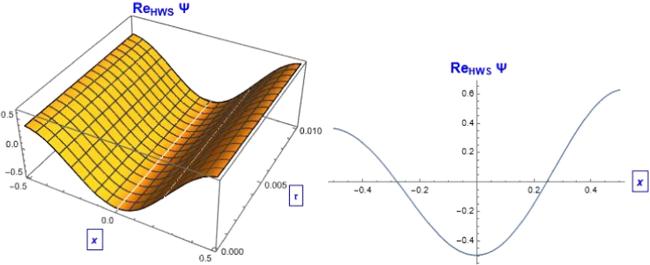
Figure 13. The HW numerical solution behavior of the Re. part of equation ( |
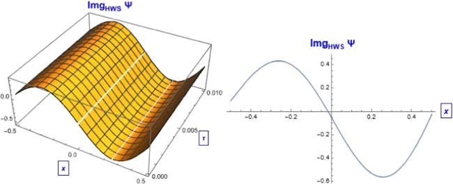
Figure 14. The HW numerical solution behavior to the Im. part of equation ( |
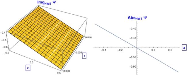
Figure 15. The 2D and 3D soliton HWN solution behavior of $\left|{\rm{\Psi }}\right|$ equations ( |
Using equation (71 ) in equation (67 ), then the Haar wavelet solution of equation (62 ) is
$\begin{eqnarray}\begin{array}{rcl}u\left(\zeta \right) & = & -\displaystyle \frac{1}{2}-\displaystyle \frac{1}{4}\zeta +{a}_{1}{R}_{1}\left(\zeta \right)+{a}_{2}{R}_{2}\left(\zeta \right)\\ & & +{a}_{3}{R}_{3}\left(\zeta \right)+{a}_{4}{R}_{4}\left(\zeta \right)=-\displaystyle \frac{1}{2}-\displaystyle \frac{1}{4}\zeta \\ & & -0.00279276\,{R}_{1}\left(\zeta \right)-0.0929915\,{R}_{2}\left(\zeta \right)\\ & & -0.0262158\,{R}_{3}\left(\zeta \right)-0.0656008\,{R}_{4}\left(\zeta \right).\end{array}\end{eqnarray}$
Hence, $\begin{eqnarray*}{\rm{\Psi }}\left(x,\tau \right)=u\left(\zeta \right){{\rm{e}}}^{{\rm{i}}\eta \left(x,\tau \right)}\end{eqnarray*}$
$\begin{eqnarray}\begin{array}{l}\mathrm{Re}{\rm{\Psi }}\left(x,\tau \right)\,=\\ \left(\begin{array}{l}-0.5-0.25\left(x-\displaystyle \frac{1}{3}\tau \right)-0.00279276{R}_{1}\left[x-\displaystyle \frac{1}{3}\tau \right]\\ -0.0929915{R}_{2}\left[x-\displaystyle \frac{1}{3}\tau \right]\\ -0.026216{R}_{3}\left[x-\displaystyle \frac{1}{3}\tau \right]-0.0656008{R}_{4}\left[x-\displaystyle \frac{1}{3}\tau \right]\end{array}\right)\\ \,\times \,\cos \left[6x+\tau +0.1\right],\end{array}\end{eqnarray}$
$\begin{eqnarray}\begin{array}{c}\rm{Im}{\rm{\Psi }}\left(x,\tau \right)\,=\\ \left(\begin{array}{c}-0.5-0.00279276{R}_{1}\left[x-\displaystyle \frac{1}{3}\tau \right]\\ -0.0929915{R}_{2}\left[x-\displaystyle \frac{1}{3}\tau \right]-0.25\left(x-\displaystyle \frac{1}{3}\tau \right)\\ -0.02622{R}_{3}\left[x-\displaystyle \frac{1}{3}\tau \right]-0.065601{R}_{4}\left[x-\displaystyle \frac{1}{3}\tau \right]\end{array}\right)\\ \,\times \,\sin \left[6x+\tau +0.1\right].\end{array}\end{eqnarray}$
4.4. The numerical solution using the HWNS corresponding to the exact solution derived by GKS (imaginary part)
For the imaginary part equation (12 ) with the following28 ), which has the following initial conditions76 ) in the form78 ) twice from $0\to \zeta $ we obtain78 )–(80 ) into equation (76 ) we get81 ) at the collocation points given in equation (57 ) we get
$\begin{eqnarray}\begin{array}{l}\delta =R={g}_{c}={g}_{R}={\gamma }_{R}={n}_{R}=w=k=1,\\ P=\displaystyle \frac{-89}{16},{\gamma }_{c}=-\displaystyle \frac{1}{2},q=-\displaystyle \frac{5}{4},\end{array}\end{eqnarray}$
becomes $\begin{eqnarray}\displaystyle \frac{1}{4}u^{\prime\prime} \left(\zeta \right)-\displaystyle \frac{3}{4}u^{\prime} \left(\zeta \right)+\displaystyle \frac{1}{2}u\left(\zeta \right)-\displaystyle \frac{1}{2}{u}^{3}\left(\zeta \right)=0,\end{eqnarray}$
whose exact solution derived by GKS is equation ( $\begin{eqnarray}u\left(0\right)=-\displaystyle \frac{1}{2},u^{\prime} \left(0\right)=-\displaystyle \frac{1}{4}.\end{eqnarray}$
The HWNS considers the solution of equation ( $\begin{eqnarray}u^{\prime\prime} \left(\zeta \right)=\displaystyle \sum _{i=1}^{2M}{a}_{i}{h}_{i}\left(\zeta \right).\end{eqnarray}$
By integrating equation ( $\begin{eqnarray}\displaystyle \begin{array}{rcl}u^{\prime} \left(\zeta \right) & = & \sum _{i=1}^{2M}{a}_{i}{p}_{i}\left(\zeta \right)+u^{\prime} \left(0\right)\\ & = & -\displaystyle \frac{1}{4}+\sum _{i=1}^{2M}{a}_{i}{p}_{i}\left(\zeta \right),\end{array}\end{eqnarray}$
$\begin{eqnarray}\displaystyle \begin{array}{rcl}u\left(\zeta \right) & = & \displaystyle \sum _{i=1}^{2M}{a}_{i}{Q}_{i}\left(\zeta \right)-\displaystyle \frac{1}{4}\zeta +u\left(0\right)\\ & = & -\displaystyle \frac{1}{2}-\displaystyle \frac{1}{4}\zeta +\displaystyle \sum _{i=1}^{2M}{a}_{i}{Q}_{i}\left(\zeta \right).\end{array}\end{eqnarray}$
By substituting from equations ( $\begin{eqnarray}\begin{array}{c}\displaystyle \frac{1}{4}\displaystyle \sum _{i=1}^{2M}{a}_{i}{h}_{i}\left(\zeta \right)-\displaystyle \frac{3}{4}\left(-\displaystyle \frac{1}{4}+\displaystyle \sum _{i=1}^{2M}{a}_{i}{P}_{i}\left(\zeta \right)\right)\\ \,+\,\displaystyle \frac{1}{2}\left(-\displaystyle \frac{1}{2}-\displaystyle \frac{1}{4}\zeta +\displaystyle \sum _{i=1}^{2M}{a}_{i}{Q}_{i}\left(\zeta \right)\right)\\ \,-\,\displaystyle \frac{1}{2}{\left(-\displaystyle \frac{1}{2}-\displaystyle \frac{1}{4}\zeta +\displaystyle \sum _{i=1}^{2M}{a}_{i}{Q}_{i}\left(\zeta \right)\right)}^{3}=0.\end{array}\end{eqnarray}$
Satisfying equation ( $\begin{eqnarray}\begin{array}{c}\displaystyle \frac{1}{4}\displaystyle \sum _{i=1}^{2M}{a}_{i}{h}_{i}\left({\zeta }_{l}\right)\,-\displaystyle \frac{3}{4}\left(-\displaystyle \frac{1}{4}+\displaystyle \sum _{i=1}^{2M}{a}_{i}{P}_{i}\left({\zeta }_{l}\right)\right)\\ \,+\,\displaystyle \frac{1}{2}\left(-\displaystyle \frac{1}{2}-\displaystyle \frac{1}{4}{\zeta }_{l}+\displaystyle \sum _{i=1}^{2M}{a}_{i}{Q}_{i}\left({\zeta }_{l}\right)\right)\\ \,-\,\displaystyle \frac{1}{2}{\left(-\displaystyle \frac{1}{2}-\displaystyle \frac{1}{4}{\zeta }_{l}+\displaystyle \sum _{i=1}^{2M}{a}_{i}{Q}_{i}\left({\zeta }_{l}\right)\right)}^{3}=0\,{,}\,l=1,2,\mathrm{..}.,2M.\end{array}\end{eqnarray}$
Let the parameter $J=1\to M={2}^{J}=2\to 2M=4\,\to l=1,2,3,4$ in equation (82 )83 ), at collocation points ${\zeta }_{l}\,=\displaystyle \frac{l-0.5}{2M}=\displaystyle \frac{l-0.5}{4},l=1,2,3,4$, surrenders to a system of unknowns ${a}_{i},i=1,2,3,4,$ and its solution is84 ) is
$\begin{eqnarray}\begin{array}{c}\displaystyle \frac{1}{4}\displaystyle \sum _{i=1}^{4}{a}_{i}{h}_{i}\left({\zeta }_{l}\right)-\displaystyle \frac{3}{4}\left(-\displaystyle \frac{1}{4}+\displaystyle \sum _{i=1}^{4}{a}_{i}{P}_{i}\left({\zeta }_{l}\right)\right)\\ \,+\,\displaystyle \frac{1}{2}\left(-\displaystyle \frac{1}{2}-\displaystyle \frac{1}{4}{\zeta }_{l}+\displaystyle \sum _{i=1}^{4}{a}_{i}{Q}_{i}\left({\zeta }_{l}\right)\right)\\ \,-\,\displaystyle \frac{1}{2}{\left(-\displaystyle \frac{1}{2}-\displaystyle \frac{1}{4}{\zeta }_{l}+\displaystyle \sum _{i=1}^{4}{a}_{i}{Q}_{i}\left({\zeta }_{l}\right)\right)}^{3}=0,l=1,2,3,4.\end{array}\end{eqnarray}$
Equation ( $\begin{eqnarray}\begin{array}{rcl}{a}_{1} & = & 0.0771199,\\ {a}_{2} & = & -0.0397252,\\ {a}_{3} & = & -0.0172571,\\ {a}_{4} & = & -0.0252802.\end{array}\end{eqnarray}$
Then, the Haar wavelet solution of equation ( $\begin{eqnarray}\begin{array}{rcl}u\left(\zeta \right) & = & -\displaystyle \frac{1}{2}-\displaystyle \frac{1}{4}\zeta +{a}_{1}{Q}_{1}\left(\zeta \right)\\ & & +\,{a}_{2}{Q}_{2}\left(\zeta \right)+{a}_{3}{Q}_{3}\left(\zeta \right)+{a}_{4}{Q}_{4}\left(\zeta \right)\\ & = & -\displaystyle \frac{1}{2}-\displaystyle \frac{1}{4}\zeta 0.0771199{Q}_{1}\left(\zeta \right)-0.0397252{Q}_{2}\left(\zeta \right)\\ & & -\,0.0172571{Q}_{3}\left(\zeta \right)-0.0252802{Q}_{4}\left(\zeta \right),\end{array}\end{eqnarray}$
$\begin{eqnarray*}{\rm{Q}}{\rm{\Psi }}\left(x,\tau \right)=u\left(\zeta \right){{\rm{e}}}^{{\rm{i}}\eta \left(x,\tau \right)}\end{eqnarray*}$
$\begin{eqnarray}\begin{array}{l}\mathrm{Re}{\rm{\Psi }}\left(x,\tau \right)\,=\\ \left(\begin{array}{l}-\displaystyle \frac{1}{2}-\displaystyle \frac{1}{4}\left(x+\tau \right)+\,0.0771199{Q}_{1}\left(x+\tau \right)\\ -0.0397252{Q}_{2}\left(x+\tau \right)\\ -0.0172571{Q}_{3}\left(x+\tau \right)-0.0252802{Q}_{4}\left(x+\tau \right)\end{array}\right)\\ \,\times \,\cos \left[-\displaystyle \frac{5}{4}x+\tau +0.1\right],\end{array}\end{eqnarray}$
and $\begin{eqnarray}\begin{array}{c}\rm{Im}{\rm{\Psi }}\left(x,\tau \right)\,=\\ \left(\begin{array}{c}-\displaystyle \frac{1}{2}-\displaystyle \frac{1}{4}\left(x+\tau \right)+\,0.0771199{Q}_{1}\left(x+\tau \right)\\ -0.0397252{Q}_{2}\left(x+\tau \right)\\ -0.0172571{Q}_{3}\left(x+\tau \right)-0.0252802{Q}_{4}\left(x+\tau \right)\end{array}\right)\\ \times \,\sin \left[-\displaystyle \frac{5}{4}x+\tau +0.1\right].\end{array}\end{eqnarray}$
4.5. The numerical solution by the HWNS corresponding to the exact solution derived by the $\left(\displaystyle \frac{G^{\prime} }{G}\right)$-expansion scheme (real part)
According to $\left(\displaystyle \frac{G^{\prime} }{G}\right)$ the real part of equation (11 ) with the following values40 ), which has the following initial conditions89 ) takes the form91 ) three times from $0\to \zeta $ 91 )–(94 ) in equation (89 ) one can get95 ) at the collocation points ${\zeta }_{l}=\displaystyle \frac{l-0.5}{2M}=\displaystyle \frac{l-0.5}{4},l=1,2,3,4$, we obtain a system in the unknowns ${a}_{i},i=1,2,3,4,$ and by solving this system we find
$\begin{eqnarray}\begin{array}{l}R=P=q={g}_{c}={g}_{R}={\gamma }_{R}={n}_{R}=w=k=1,\\ \delta =\displaystyle \frac{-10}{27},{\gamma }_{c}=\displaystyle \frac{2}{5},\end{array}\end{eqnarray}$
becomes $\begin{eqnarray}\displaystyle \frac{1}{2}u^{\prime\prime\prime} \left(\zeta \right)-\displaystyle \frac{7}{18}u^{\prime} \left(\zeta \right)-3u^{\prime} \left(\zeta \right){u}^{2}\left(\zeta \right)-\displaystyle \frac{1}{9}u\left(\zeta \right)+{u}^{3}\left(\zeta \right)=0,\end{eqnarray}$
whose exact solution derived by $\left(\displaystyle \frac{G^{\prime} }{G}\right)$ is equation ( $\begin{eqnarray}u\left(0\right)=\displaystyle \frac{1}{6},u^{\prime} \left(0\right)=-\displaystyle \frac{1}{12},u^{\prime\prime} \left(0\right)=\displaystyle \frac{1}{18}.\end{eqnarray}$
The Haar wavelet solution of equation ( $\begin{eqnarray}u^{\prime\prime\prime} \left(\zeta \right)=\displaystyle \sum _{i=1}^{2M}{a}_{i}{h}_{i}\left(\zeta \right).\end{eqnarray}$
To reach $u\left(\zeta \right)$, we integrate equation ( $\begin{eqnarray}u^{\prime\prime} \left(\zeta \right)=\displaystyle \sum _{i=1}^{2M}{a}_{i}{p}_{i}\left(\zeta \right)+u^{\prime\prime} \left(0\right)=\displaystyle \frac{1}{18}+\displaystyle \sum _{i=1}^{2M}{a}_{i}{p}_{i}\left(\zeta \right),\end{eqnarray}$
$\begin{eqnarray}\displaystyle \begin{array}{rcl}u^{\prime} \left(\zeta \right) & = & \sum _{i=1}^{2M}{a}_{i}{Q}_{i}\left(\zeta \right)+\displaystyle \frac{1}{18}\zeta +u^{\prime} \left(0\right)\\ & = & -\displaystyle \frac{1}{12}+\displaystyle \frac{1}{18}\zeta +\sum _{i=1}^{2M}{a}_{i}{Q}_{i}\left(\zeta \right),\end{array}\end{eqnarray}$
$\begin{eqnarray}\displaystyle \begin{array}{rcl}u\left(\zeta \right) & = & \displaystyle \sum _{i=1}^{2M}{a}_{i}{R}_{i}\left(\zeta \right)+\displaystyle \frac{1}{36}{\zeta }^{2}-\displaystyle \frac{1}{12}\zeta +u\left(0\right)\\ & = & \displaystyle \frac{1}{36}{\zeta }^{2}-\displaystyle \frac{1}{12}\zeta +\displaystyle \frac{1}{6}+\displaystyle \sum _{i=1}^{2M}{a}_{i}{R}_{i}\left(\zeta \right).\end{array}\end{eqnarray}$
Using equations ( $\begin{eqnarray}\begin{array}{c}\displaystyle \frac{1}{2}\displaystyle \sum _{i=1}^{2M}{a}_{i}{h}_{i}\left(\zeta \right)-\displaystyle \frac{7}{18}\left(-\displaystyle \frac{1}{12}+\displaystyle \frac{1}{18}\zeta +\displaystyle \sum _{i=1}^{2M}{a}_{i}{Q}_{i}\left(\zeta \right)\right)\\ \,-\,\displaystyle \frac{1}{9}\left(\displaystyle \frac{1}{36}{\zeta }^{2}-\displaystyle \frac{1}{12}\zeta +\displaystyle \frac{1}{6}+\displaystyle \sum _{i=1}^{2M}{a}_{i}{R}_{i}\left(\zeta \right)\right)\\ \,-\,3\left(-\displaystyle \frac{1}{12}+\displaystyle \frac{1}{18}\zeta +\displaystyle \sum _{i=1}^{2M}{a}_{i}{Q}_{i}\left(\zeta \right)\right)\\ \,\times \,{\left(\displaystyle \frac{1}{36}{\zeta }^{2}-\displaystyle \frac{1}{12}\zeta +\displaystyle \frac{1}{6}+\displaystyle \sum _{i=1}^{2M}{a}_{i}{R}_{i}\left(\zeta \right)\right)}^{2}\\ \,+\,{\left(\displaystyle \frac{1}{36}{\zeta }^{2}-\displaystyle \frac{1}{12}\zeta +\displaystyle \frac{1}{6}+\displaystyle \sum _{i=1}^{2M}{a}_{i}{R}_{i}\left(\zeta \right)\right)}^{3}=0\,.\end{array}\end{eqnarray}$
Putting the level of resolution $J=1\to \,M={2}^{J}=2\to 2M=4\to l=1,2,3,4,$ satisfying equation ( $\begin{eqnarray}\begin{array}{rcl}{a}_{1} & = & -0.0250399,\\ {a}_{2} & = & -0.0067265,\\ {a}_{3} & = & -0.00423359,\\ {a}_{4} & = & -0.00253455.\end{array}\end{eqnarray}$
The Haar wavelet solution of equation (89 ) is
$\begin{eqnarray}\begin{array}{rcl}u\left(\zeta \right) & = & \displaystyle \frac{1}{36}{\zeta }^{2}-\displaystyle \frac{1}{12}\zeta +\displaystyle \frac{1}{6}+{a}_{1}{R}_{1}\left(\zeta \right)+{a}_{2}{R}_{2}\left(\zeta \right)\\ & & +\,{a}_{3}{R}_{3}(\zeta )+{a}_{4}{R}_{4}\left(\zeta \right)\\ & = & \displaystyle \frac{1}{36}{\zeta }^{2}-\displaystyle \frac{1}{12}\zeta +\displaystyle \frac{1}{6}\\ & & -\,0.0250399\,{R}_{1}\left(\zeta \right)-0.0067265\,{R}_{2}\left(\zeta \right)\\ & & -\,0.00423359{R}_{3}\left(\zeta \right)-0.00253455\,{R}_{4}\left(\zeta \right).\end{array}\end{eqnarray}$
And hence, ${\rm{\Psi }}\left(x,\tau \right)=u\left(\zeta \right){{\rm{e}}}^{{\rm{i}}\eta \left(x,\tau \right)}$, from which we get $\begin{eqnarray}\begin{array}{l}\mathrm{Re}{\rm{\Psi }}(x,\tau )\,=\\ \left(\begin{array}{l}\displaystyle \frac{1}{36}{\left(x+\tau \right)}^{2}+\displaystyle \frac{1}{6}-0.0250399\,{R}_{1}\left(x+\tau \right)\\ -0.0067265\,{R}_{2}\left(x+\tau \right)-0.0042336{R}_{3}\left(x+\tau \right)\\ -0.00253455\,{R}_{4}\left(x+\tau \right)-\displaystyle \frac{1}{12}\left(x+\tau \right)\end{array}\right)\\ \,\times \,\cos \left[x-\displaystyle \frac{10}{27}\tau +0.1\right],\end{array}\end{eqnarray}$
$\begin{eqnarray}\begin{array}{c}\rm{Im}{\rm{\Psi }}\left(x,\tau \right)\,=\\ \left(\begin{array}{c}\displaystyle \frac{1}{36}{\left(x+\tau \right)}^{2}+\displaystyle \frac{1}{6}-0.0250399\,{R}_{1}\left(x+\tau \right)\\ -0.0067265\,{R}_{2}\left(x+\tau \right)-0.00423359{R}_{3}\left(x+\tau \right)\\ -0.00253455\,{R}_{4}\left(x+\tau \right)-\displaystyle \frac{1}{12}\left(x+\tau \right)\end{array}\right)\\ \,\times \,\sin \left[x-\displaystyle \frac{10}{27}\tau +0.1\right].\end{array}\end{eqnarray}$
4.6. The numerical solution by the HWNS corresponding to the exact solution derived by the $\left(\displaystyle \frac{G^{\prime} }{G}\right)$-expansion scheme (imaginary part)
The imaginary part equation (12 ) with the following47 ), which has the following initial conditions101 ) in the form103 ) twice from $0\to \zeta $ to obtain $u\left(\zeta \right)$ 103 )–(105 ) into equation (101 ) we get
$\begin{eqnarray}\begin{array}{l}\delta =R={g}_{R}={\gamma }_{c}={\gamma }_{R}={n}_{R}=w=k=P=q=1,\\ {g}_{c}=\displaystyle \frac{11}{2},\end{array}\end{eqnarray}$
is reduced to $\begin{eqnarray}\displaystyle \frac{5}{2}u^{\prime\prime} \left(\zeta \right)-\displaystyle \frac{5}{2}u\left(\zeta \right)-5{u}^{3}\left(\zeta \right)=0,\end{eqnarray}$
whose exact solution derived by $\left(\displaystyle \frac{G^{\prime} }{G}\right)$ is equation ( $\begin{eqnarray}u\left(0\right)=i\sqrt{2},u^{\prime} \left(0\right)=0.\end{eqnarray}$
The HWNS considers the solution of equation ( $\begin{eqnarray}u^{\prime\prime} \left(\zeta \right)=\displaystyle \sum _{i=1}^{2M}{a}_{i}{h}_{i}\left(\zeta \right).\end{eqnarray}$
By integrating equation ( $\begin{eqnarray}u^{\prime} \left(\zeta \right)=\displaystyle \sum _{i=1}^{2M}{a}_{i}{p}_{i}\left(\zeta \right)+u^{\prime} \left(0\right)=\displaystyle \sum _{i=1}^{2M}{a}_{i}{p}_{i}\left(\zeta \right),\end{eqnarray}$
$\begin{eqnarray}u\left(\zeta \right)=\displaystyle \sum _{i=1}^{2M}{a}_{i}{Q}_{i}\left(\zeta \right)+u\left(0\right)={\rm{i}}\sqrt{2}+\displaystyle \sum _{i=1}^{2M}{a}_{i}{Q}_{i}\left(\zeta \right).\end{eqnarray}$
Inserting equations ( $\begin{eqnarray}\begin{array}{c}\displaystyle \frac{5}{2}\displaystyle \sum _{i=1}^{2M}{a}_{i}{h}_{i}\left(\zeta \right)-\displaystyle \frac{5}{2}\left(i\sqrt{2}+\displaystyle \sum _{i=1}^{2M}{a}_{i}{Q}_{i}\left(\zeta \right)\right)\\ \,-\,5{\left({\rm{i}}\sqrt{2}+\displaystyle \sum _{i=1}^{2M}{a}_{i}{Q}_{i}\left(\zeta \right)\right)}^{3}=0.\end{array}\end{eqnarray}$
Taking the level of resolution $J=1,$ satisfying equation (106 ) at the collocation points ${\zeta }_{l}=\displaystyle \frac{l-0.5}{2M}\,=\displaystyle \frac{l-0.5}{4},l=1,2,3,4$, a system in the unknowns ${a}_{i},i=1,2,3,4$ is obtained. Solving this system, we get
$\begin{eqnarray}\begin{array}{rcl}{a}_{1} & = & 0.175656{\rm{i}},\\ {a}_{2} & = & -2.84584{\rm{i}},\\ {a}_{3} & = & -1.23671{\rm{i}},\\ {a}_{4} & = & -1.074{\rm{i}}.\end{array}\end{eqnarray}$
Then the Haar wavelet solution of equation (110 ) is:
$\begin{eqnarray}\begin{array}{rcl}u\left(\zeta \right) & = & {\rm{i}}\sqrt{2}+0.175656{\rm{i}}{Q}_{1}\left[\zeta \right]-2.84584{\rm{i}}{Q}_{2}\left[\zeta \right]\\ & & -\,1.23671{\rm{i}}{Q}_{3}\left[\zeta \right]-1.074{\rm{i}}{Q}_{4}\left[\zeta \right].\end{array}\end{eqnarray}$
And hence, ${\rm{\Psi }}\left(x,\tau \right)=u\left(\zeta \right){{\rm{e}}}^{{\rm{i}}\eta \left(x,\tau \right)}$, from which we get $\begin{eqnarray}\begin{array}{l}\mathrm{Re}{\rm{\Psi }}(x,\tau )\,=\\ -\,\left(\begin{array}{l}\sqrt{2}+0.175656{Q}_{1}\left[x+\tau \right]-2.84584{Q}_{2}\left[x+\tau \right]\\ -1.23671{Q}_{3}\left[x+\tau \right]-1.074{Q}_{4}\left[x+\tau \right]\end{array}\right)\\ \,\times \,\sin \left[x+\tau +0.1\right],\end{array}\end{eqnarray}$
$\begin{eqnarray}\begin{array}{c}\rm{Im}{\rm{\Psi }}\left(x,\tau \right)\,=\\ \left(\begin{array}{c}\sqrt{2}+0.175656{Q}_{1}\left[x+\tau \right]-2.84584{Q}_{2}\left[x+\tau \right]\\ -1.23671{Q}_{3}\left[x+\tau \right]-1.074{Q}_{4}\left[x+\tau \right]\end{array}\right)\\ \,\times \,\cos \left[x+\tau +0.1\right].\end{array}\end{eqnarray}$
5. Conclusion
In this paper, we succeeded in deriving diverse enormous soliton solutions to the Gross–Pitaevskii equation, which describes the dynamics of two dark solitons in a polarization condensate under non-resonant pumping, analytically for the first time using the generalized Kudryashov method and the (G’/G)-method. The extracted solutions in the framework of these two suggested schemes appear in forms that include dark, bright, combined bright-shaped and dark-shaped soliton solutions, hyperbolic function soliton solutions, singular shaped soliton solutions and other rational soliton solutions. Moreover, the Haar wavelet numerical method, which is one of the famous techniques in numerical methods, has been utilized to explore the numerical solutions for all realized soliton solutions by the above two techniques. The 2D and 3D graphs have been designed utilizing the Mathematica program and the figures simulations have been configured to show the agreement range between the soliton solutions and the numerical solutions, which corresponded perfectly in figures [1–23]. Our results are new compared with [22] who used the variational approach and analytically derived the time evolution equations for the soliton parameters and presented the first analytical result on the two-dark soliton problem in the context of a polarization Bose–Einstein Condensates formed under non-resonant pumping by solving the dissipative Gross–Pitaevskii equation that compares this analytical result with the numerical solutions for the trajectory of two solitons directly obtained from the dissipative Gross–Pitaevskii equation. Our realized analytical solutions and their corresponding numerical solutions have not been achieved before.
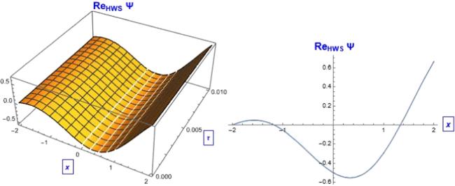
Figure 16. The numerical solution behavior to equation ( |
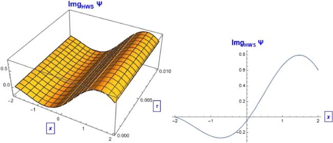
Figure 17. The numerical solution behavior to equation ( |
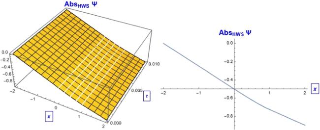
Figure 18. The 2D and 3D soliton HWN solution behavior of $\left|{\rm{\Psi }}\right|$ equations ( |
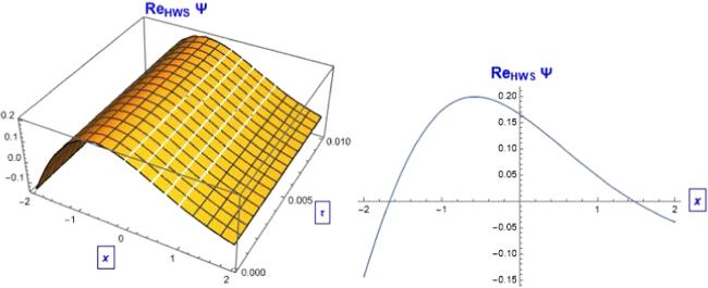
Figure 19. The numerical solution behavior to the Re. part of equation ( |
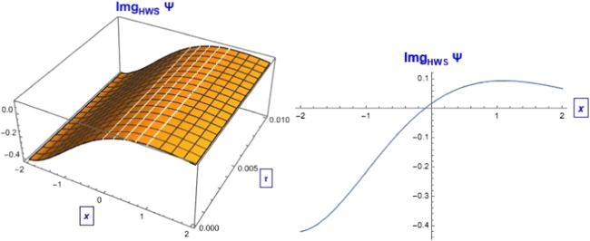
Figure 20. The numerical solution behavior to the Im. part of equation ( |
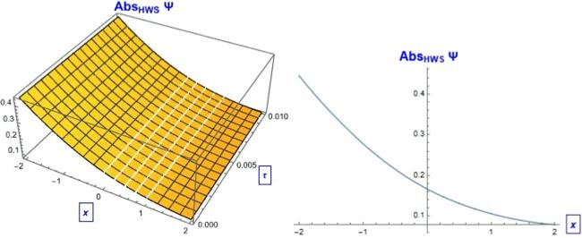
Figure 21. The 2D and 3D soliton HWN solution behavior of $\left|{\rm{\Psi }}\right|$ equation ( |
Figure 22. The numerical solution behavior to the Re. part of equation ( |
Figure 23. The numerical solution behavior to the Im. part of equation ( |