


1. Introduction
Quantum information technology exploits various quantum properties, such as quantum superposition, quantum entanglement, etc, to provide more powerful information processing capabilities [1]. Quantum algorithms, such as Shor’s factoring algorithm [2, 3], Grover’s searching algorithm [4] and the Harrow–Hassidim–Lloyd quantum algorithm for solving linear equations [5] display better quantum speed-up than their classical counterparts. In addition, various quantum communication protocols have been designed based on quantum entanglement including quantum teleportation [6, 7], quantum dense coding [8], quantum key distribution [9, 10] and quantum secret sharing [11, 12]. These protocols provide us with more flexible and secure communication methods [13]. Some of them have been commercialized and begun to provide services to individuals and institutions [14, 15].
While quantum theory has advantages in processing information, it also has some limitations, which are characterized by a branch of no-go theorems such as the no-cloning theorem [16–18], no-broadcasting theorem [19], no-deleting theorem [20] and no-hiding theorem [21]. Recently, Modi et al proposed the concept of quantum information masking (QIM) and thus discovered a new no-go theorem called the no-masking theorem, which claims that it is impossible to mask an arbitrary quantum state into a bipartite quantum entangled system [22].
QIM has attracted extensive research interest. It is found that the maximal set of maskable states is hyperdisks when masking quantum states into a bipartite quantum system [22–24]. Different from many no-go theorems, it is proved that an arbitrary set of quantum states can be masked into a multipartite quantum system [25]. To avoid the collusion that some participants would reveal the information about the encoded quantum states, a more generalized definition of k-uniform masking was proposed [26]. Similar to quantum cloning, the probabilistic or approximate masking that allows for some imperfections of masking are also investigated [27, 28]. Beyond that, it has been shown that QIM has a close relationship with other quantum information processing tasks such as quantum secret sharing [11, 12, 26], quantum error-correction codes [26, 29] and quantum bit commitment [22, 30–33]. Complementing these theoretical advancements, experimental demonstrations of quantum information masking have materialized, with Liu et al executing masking operations using photonic systems and validating key theoretical predictions [34]. In parallel, Zhang et al pioneered the experimental realization of masking in high-dimensional systems [35], propelling the field forward with tangible evidence of masking’s practical feasibility. These collective efforts have significantly bolstered the theoretical and experimental foundations of quantum information masking, underscoring its pivotal role in the broader landscape of quantum information processing.
To use QIM, we first need to design maskers that meet the requirements for different tasks. Routinely, analytical algebra methods have been developed to obtain quantum maskers [29, 36]. However, these methods become difficult and even unsolvable as the system grows, due to the ‘exponential explosion’ on the dimension of the system. To circumvent the ‘exponential explosion’, we propose a variational quantum algorithm to design quantum maskers. Our algorithm is a hybrid quantum–classical model, where the quantum device is parameterized to realize quantum maskers and the classical device is responsible for evaluating and optimizing the quantum device. By carefully designing the loss function, it can be used to characterize the performance of quantum maskers. Our algorithm will return a perfect masker if it exists, otherwise, the masker returned is still optimal. To speed up the design process and reduce quantum resources on quantum state preparations and measurements, quantum parallelism is utilized to evaluate the loss function.
2. Preliminary
QIM aims to encode quantum information into a multipartite system so that the original quantum information is completely unknown to local subsystems. Li and Wang generalized the definition of masking to multipartite scenarios and proved that an arbitrary quantum state can be masked when more participants are allowed [25]. To avoid collusion of some participants, Shi et al further generalized QIM to k-uniform QIM [26]. Let us briefly review and rephrase it [37].
First, let us denote a d-dimension Hilbert space corresponding to a quantum system X by ${{ \mathcal H }}_{X}$. We use ${ \mathcal Q }{ \mathcal S }={\{({p}_{i},| {\psi }_{i}\rangle )\}}_{i=1}^{n}$ to denote a quantum information source that generates a pure state ∣ψi⟩ with probability pi. We also use S to denote the state set ${\{| {\psi }_{i}\rangle \}}_{i=1}^{n}$. For brevity, we use [N] to denote the set {1, 2, ⋯ , N}. Then, QIM is defined as follows.
Definition 1. Given ${ \mathcal Q }{ \mathcal S }={\{({p}_{i},| {\psi }_{i}\rangle )\}}_{i=1}^{n}$ labeled A, if there exists a quantum operation M that maps any pure state $| {\psi }_{i}\rangle \in S\subset {{ \mathcal H }}_{A}$ to a state $| {{\rm{\Psi }}}_{i}\rangle \in {\otimes }_{l=1}^{N}{{ \mathcal H }}_{{B}_{l}}$ so that all the marginal states of arbitrary k subsystems are identical, i.e. for all ${l}_{1}\lt {l}_{2}\lt \,\cdots \,\lt {l}_{k}\in [N]$,
$\begin{eqnarray}{\sigma }_{i}^{{B}_{{l}_{1}{l}_{2}\cdots {l}_{k}}}\equiv {\mathrm{Tr}}_{{B}_{{l}_{1}{l}_{2}\cdots {l}_{k}}^{c}}(| {{\rm{\Psi }}}_{i}{\rangle }_{B}\langle {{\rm{\Psi }}}_{i}{| }_{B}),\end{eqnarray}$
are independent of $| {\psi }_{i}\rangle $, and we say that the quantum information contained in $| {\psi }_{i}\rangle $ is k-uniformly masked into N subsystems by M, and M is a 1-to-N and k-uniform masker denoted by (N,k) masker. Here, ${B}_{{l}_{1}{l}_{2}\cdots {l}_{k}}^{c}$ denotes the complementary set of $\{{B}_{{l}_{1}},{B}_{{l}_{2}},\cdots {B}_{{l}_{k}}\}$ over $\{{B}_{1},{B}_{2},\cdots {B}_{N}\}$. We say M is a universal masker if it can mask all pure states in ${{ \mathcal H }}_{A}$.For a (N,k) masker, it demands that all the marginal states of k subsystems should be independent of input states. This implies that a total of $\left(\displaystyle \genfrac{}{}{0em}{}{N}{k}\right)\equiv \tfrac{N!}{k!(N-k)!}$ marginal subsystems need to be evaluated. This is a huge amount of work, especially when N is large and k is approximately N/2.
Given ${ \mathcal Q }{ \mathcal S }$, N and k, a perfect (N,k) masker can completely mask the quantum source. However, in some cases, perfect maskers may not exist. For these cases, optimal maskers that mask original information as much as possible are practical and useful. Thus, our purpose is to design optimal maskers. For two quantum sources, even if they produce the same set of quantum states, the optimal maskers are usually different due to the different probabilities. This further increases the difficulty of designing quantum maskers.
3. Variational quantum algorithm for designing maskers
In this section, we introduce our variational quantum algorithm for designing maskers in detail. For simplicity, the rest of the discussion will be limited to qubit masking unless otherwise stated. For higher-dimensional cases, they can be simulated with qubits.
3.1. Parameterized quantum masker
First, in our algorithm, a quantum masker is implemented by a parameterized quantum circuit (PQC) M(θ) with adjustable parameters θ = (θ1, θ2, ⋯ ), as shown in figure 1. PQCs are widely used in variational quantum algorithms due to their expressivity, robustness and ease of implementation [38–42]. In the field of quantum machine learning, PQCs are an important way to realize quantum neural networks [43–45]. We call these kinds of maskers variational quantum maskers (VQMs).
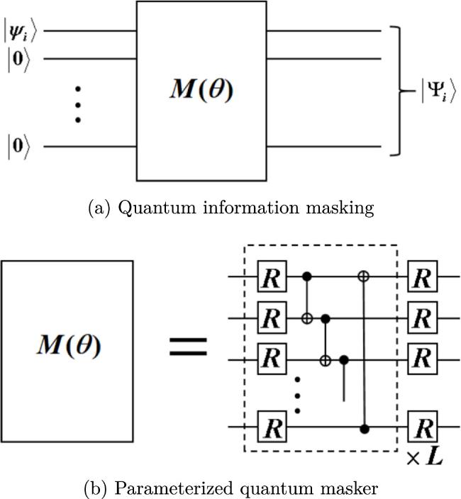
Figure 1. Illustration of quantum information masking and a parameterized quantum circuit model for a masker. R is a single-qubit rotation operation that can be parameterized by three real numbers that are not expressed explicitly. |
VQMs can be constructed in various forms, depending on the specific research or the constraints of the quantum hardware [46, 47]. A well-designed ansatz, which is a structural implementation of a VQM, can significantly accelerate convergence to more accurate solutions. The ingenious design of ansatzes for PQCs lies outside the purview of this paper [48–50]. From the perspective of theoretical research, a common PQC scheme is shown in figure 1(b), which exhibits desirable properties [51]. Here, the VQM consists of L basic units, each of which is further composed of single-qubit operations {R} and controlled-NOT gates. Each R is parameterized with three adjustable rotation angles α, β and γ, that is R(α, β, γ) = e−iZα/2e−iYβ/2e−iZγ/2, where X, Y and Z are Pauli operators [38]. The role of controlled-NOT gates is to introduce quantum entanglement between qubits. Our task is to find the optimal parameters so that the PQC behaves as an optimal masker. This is addressed by a hybrid quantum–classical model.
3.2. Loss function
To optimize parameters, we design a loss function according to definition 1 ,
$\begin{eqnarray}L(\theta )=\displaystyle \frac{1}{{ \mathcal N }}\displaystyle \sum _{l}\displaystyle \sum _{i,j=1}^{n}{p}_{i}{p}_{j}S({\sigma }_{i}^{{B}_{l}},{\sigma }_{j}^{{B}_{l}}),\end{eqnarray}$
where ${ \mathcal N }=2\left(\displaystyle \genfrac{}{}{0em}{}{N}{k}\right)$ is the standardized coefficient. S(σ1, σ2) is a similarity function that measures the similarity between σ1 and σ2. For ease of notation, here we use the composite index l = {l1, l2, ⋯ , lk} to mark k subsystems. It is required that S(σ1, σ2) ≥ 0 holds for any σ1 and σ2. The equation is true if and only if σ1 = σ2. Thus, L(θ) is equal to the lower bound 0 when all states of k subsystems are identical (independent of input states), which implies the quantum information carried by input states is perfectly masked. Conversely, the greater the value of L(θ), the worse the performance of the masker. Therefore, loss value can be used as a measure of the performance of a masker.The similarity measurement has a wide variety of definitions among math and machine learning practitioners [52]. In this study, we use the squared Hilbert–Schmidt distance as a measure of similarity [53, 54]. The Hilbert–Schmidt distance between σ1 and σ2 is defined as,A for a detailed discussion of SWAP tests.
$\begin{eqnarray}{D}_{{\rm{H}}{\rm{-}}{\rm{S}}}({\sigma }_{1},{\sigma }_{2})=\sqrt{\mathrm{Tr}\left({\left({\sigma }_{1}-{\sigma }_{2}\right)}^{\dagger }({\sigma }_{1}-{\sigma }_{2})\right)}.\end{eqnarray}$
Thus, the similarity function has the form of, $\begin{eqnarray}\begin{array}{rcl}S({\sigma }_{1},{\sigma }_{2}) & = & {D}_{{\rm{H}}{\rm{-}}{\rm{S}}}^{2}({\sigma }_{1},{\sigma }_{2})\\ & = & \mathrm{Tr}({\sigma }_{1}^{2})+\mathrm{Tr}({\sigma }_{2}^{2})-2\mathrm{Tr}({\sigma }_{1}{\sigma }_{2}).\end{array}\end{eqnarray}$
The quantity $\mathrm{Tr}({\sigma }_{1}{\sigma }_{2})$ is called the overlap between σ1 and σ2, which can be effectively estimated by SWAP tests [55, 56]. The quantum circuit of a SWAP test is shown in figure 2. See appendix 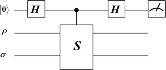
Figure 2. Diagram of the quantum circuit for the SWAP test. Here, H represents the Hadamard gate and S is the SWAP gate. By measuring the expectation value of the first qubit with respect to the Pauli-Z operator, we obtain the overlap between states $\rho$ and σ. |
Substituting equation (4 ) into (2 ), we obtain the concrete expression of the loss function as,1 )). Based on SWAP tests, each term in equation (5 ) can be evaluated, resulting in an evaluation of the loss function. As mentioned earlier, this method is extremely inefficient due to the large number of terms to be evaluated in equation (5 ), especially for large n, N and k ≈ ⌊N/2⌋. Efficient methods need to be developed.
$\begin{eqnarray}\begin{array}{rcl}L(\theta ) & = & \frac{1}{{ \mathcal N }}\displaystyle \sum _{l}\displaystyle \sum _{i,j}{p}_{i}{p}_{j}\left(\mathrm{Tr}({\sigma }_{i}^{{B}_{l}}{\sigma }_{i}^{{B}_{l}})+\mathrm{Tr}({\sigma }_{j}^{{B}_{l}}{\sigma }_{j}^{{B}_{l}})\right.\\ & & \left.-2\mathrm{Tr}({\sigma }_{i}^{{B}_{l}}{\sigma }_{j}^{{B}_{l}})\right)\\ & = & {\left(\genfrac{}{}{0em}{}{N}{k}\right)}^{-1}\displaystyle \sum _{l}\left(\displaystyle \sum _{i}{p}_{i}\mathrm{Tr}({\sigma }_{i}^{{B}_{l}}{\sigma }_{i}^{{B}_{l}})-\displaystyle \sum _{i,j}{p}_{i}{p}_{j}\mathrm{Tr}({\sigma }_{i}^{{B}_{l}}{\sigma }_{j}^{{B}_{l}})\right),\end{array}\end{eqnarray}$
where ${\sigma }_{i}^{{B}_{l}}$ is the marginal state of k subsystems labeled by composite index l (See equation (3.3. Parallel evaluation of loss function
Estimating loss functions directly requires repeating a large number of SWAP tests, consuming a lot of quantum resources and time. To speed up the process and save quantum resources, we take advantage of the technology of quantum parallelism [57]. The terms in equation (5 ) stem from two aspects, the states generated by the quantum information source and the combinations of k out of N. Let us explore how parallelism can be used to accelerate these two.
First, let us deal with the complexity that comes with quantum sources. We have shown in appendix A that ${\sum }_{i}{p}_{i}\mathrm{Tr}({\sigma }_{i}^{{B}_{l}}{\sigma }_{i}^{{B}_{l}})$ can be evaluated by using the SWAP test only once with input state ${\sigma }^{{B}_{l}}={\sum }_{i}{p}_{i}{\sigma }_{i}^{{B}_{l}}\otimes {\sigma }_{i}^{{B}_{l}}$, that is,5 ) can be rewritten as,
$\begin{eqnarray}\displaystyle \sum _{i}{p}_{i}\mathrm{Tr}({\sigma }_{i}^{{B}_{l}}{\sigma }_{i}^{{B}_{l}})=\mathrm{ST}({\sigma }^{{B}_{l}}),\end{eqnarray}$
where ST( · ) is a functional representation of the SWAP test. To clarify, ‘running the SWAP test once’ here refers to one evaluation of the overlap between two states, which requires multiple measurements, and the higher the accuracy requirement, the more measurements need to be performed. Similarly, ${\sum }_{i,j}{p}_{i}{p}_{j}\mathrm{Tr}({\sigma }_{i}^{{B}_{l}}{\sigma }_{j}^{{B}_{l}})$ can be evaluated by inputting ${\tilde{\sigma }}^{{B}_{l}}={\sum }_{i}{p}_{i}{\sigma }_{i}^{{B}_{l}}\otimes {\sum }_{j}{p}_{j}{\sigma }_{j}^{{B}_{l}}$, that is, $\begin{eqnarray}\displaystyle \sum _{i,j}{p}_{i}{p}_{j}\mathrm{Tr}({\sigma }_{i}^{{B}_{l}}{\sigma }_{j}^{{B}_{l}})=\mathrm{ST}({\tilde{\sigma }}^{{B}_{l}}).\end{eqnarray}$
Thus, equation ( $\begin{eqnarray}L(\theta )={\left(\displaystyle \genfrac{}{}{0em}{}{N}{k}\right)}^{-1}\displaystyle \sum _{l}\left(\mathrm{ST}({\sigma }^{{B}_{l}})-\mathrm{ST}({\tilde{\sigma }}^{{B}_{l}})\right).\end{eqnarray}$
Second, let us deal with the complexity that comes with combination. Due to the linearity of ST, equation (8 ) can be further rewritten asB , we give subroutines to prepare these two states deterministically.
$\begin{eqnarray}L(\theta )=\mathrm{ST}(\sigma )-\mathrm{ST}(\tilde{\sigma }),\end{eqnarray}$
where $\sigma ={\left(\displaystyle \genfrac{}{}{0em}{}{N}{k}\right)}^{-1}{\sum }_{l}{\sigma }^{{B}_{l}}$ and $\tilde{\sigma }={\left(\displaystyle \genfrac{}{}{0em}{}{N}{k}\right)}^{-1}{\sum }_{l}{\tilde{\sigma }}^{{B}_{l}}$. Therefore, the key to evaluating the loss function becomes the preparation of σ and $\tilde{\sigma }$. In appendix 3.4. Optimization
Once the loss function is effectively evaluated, the classical device can guide and update the adjustable parameters of the VQM. There are many optimization methods, including gradient-based methods and non-gradient-based methods [58]. Gradient-based methods are generally preferred due to their fast convergence speed and good precision when the parameter space is very large. However, to use gradient-based methods, the gradient information of the loss function needs to be obtained. There are different strategies to do so, and they may depend on the quantum device used. A common one is the finite difference method. Different from classical neural networks, the backpropagation algorithm is not suitable for PQCs. Fortunately, for a certain class of gradient-compatible PQCs, there are analytic methods to obtain their gradients such as ‘parameter-shift rules’ [59–61]. They express the gradient of a function as some combination of that function at two different points. However, unlike in the finite difference methods, those two points are not infinitesimally close together, but rather quite far apart. Once the gradient of loss function is obtained denoted by ∇L(θ), θ is then updated using,
$\begin{eqnarray}\theta \to \theta -{\rm{\nabla }}L(\theta ).\end{eqnarray}$
It should be noted that variational quantum algorithms are likely to encounter the barren plateau phenomenon, where the gradient vanishes [62–64]. Many fixes and workarounds have been proposed and investigated [41, 65–67]. This is beyond the scope of this paper.3.5. Complete description of variational quantum algorithm
It is time to give a complete description of the variational algorithm for designing quantum maskers. We show the pseudocode in algorithm 1 .
The subroutines of preparing states σ and $\tilde{\sigma }$ can be found in appendix B .
Algorithm 1. Variational quantum algorithm for designing quantum maskers
| Input: Quantum source ${ \mathcal Q }{ \mathcal S }$, integers N and k, number of iterations ITR; |
| Output: Optimal $M(\theta )$ |
| 1 Select a circuit ansatz $M(\theta )$ to represent a parameterized masker; |
| 2 Initialize parameters θ; |
| 3 for ${itr}=1,2,\,\cdots ,\,{ITR}$ do |
| 4 Call subroutines to prepare states σ and $\tilde{\sigma }$; |
| 5 Evaluate $\mathrm{ST}(\sigma )$ and $\mathrm{ST}(\tilde{\sigma })$ by SWAP tests, respectively; |
| 6 Calculate $L({\boldsymbol{\theta }})=\mathrm{ST}(\sigma )-\mathrm{ST}(\tilde{\sigma })$; |
| 7 Perform optimization for $L({\boldsymbol{\theta }})$ and update the parameters ${\boldsymbol{\theta }}$; |
| 8 end |
| 9 return $M(\theta )$. |
4. Consumption of quantum resources
In this section, we analyze the quantum resources required by our variational quantum algorithm in terms of the number of qubits, number of gates, and measurements. In appendix B , we have discussed that for a (N, k) quantum masker, it takes at most $2\mathrm{log}n+3N$ qubits and $O({poly}({kN},n{\mathrm{log}}^{2}n))$ gates in our algorithm. Thus, here we focus on the measurements.
To obtain the evaluation of the loss function, measurement must be performed repeatedly. A finite number of measurements inevitably introduces errors. The more times the measurement is repeated, the smaller the error in the estimate. Using SWAP tests, we need to measure $O(\tfrac{1}{{\epsilon }^{2}})$ times to guarantee that our estimate of overlap is within a precision ε > 0. Thus, in our algorithm we need $O(\tfrac{1}{{\epsilon }^{2}})$ measurements to evaluate L(θ) with an error ε > 0. However, it takes $O\left(\left(\displaystyle \genfrac{}{}{0em}{}{N}{k}\right)\tfrac{{n}^{2}}{{\epsilon }^{2}}\right)$ measurements if we directly evaluate the terms in equation (5 ). This reveals the accelerating effect of quantum parallelism.
5. Numerical simulation
To verify the feasibility of our algorithm, in this section we present the numerical simulation results. Given the challenges associated with simulating quantum algorithms on classical computers, our focus here is on the simulation of designing (2, 1) maskers. This simplified case sufficiently demonstrates the effectiveness of our algorithm. Second, for the sake of simplicity, the quantum sources to be masked are chosen as,
$\begin{eqnarray}{ \mathcal Q }{{ \mathcal S }}_{1}=\left\{\left(\displaystyle \frac{1}{4},| +\rangle \right),\left(\displaystyle \frac{1}{4},| -\rangle \right),\left(\displaystyle \frac{1}{4},| +{\rm{i}}\rangle \right),\left(\displaystyle \frac{1}{4},| -{\rm{i}}\rangle \right)\right\},\end{eqnarray}$
$\begin{eqnarray}\begin{array}{l}{ \mathcal Q }{{ \mathcal S }}_{2}=\left\{\left(\displaystyle \frac{1}{6},| +\rangle \right),\left(\displaystyle \frac{1}{6},| -\rangle \right),\left(\displaystyle \frac{1}{6},| +{\rm{i}}\rangle \right),\right.\\ \qquad \left.\,\left(\displaystyle \frac{1}{6},| -{\rm{i}}\rangle \right),\left(\displaystyle \frac{1}{6},| 0\rangle \right),\left(\displaystyle \frac{1}{6},| 1\rangle \right)\right\},\end{array}\end{eqnarray}$
$\begin{eqnarray}\begin{array}{l}{ \mathcal Q }{{ \mathcal S }}_{3}=\left\{\left(\displaystyle \frac{2}{10},| +\rangle \right),\left(\displaystyle \frac{2}{10},| -\rangle \right),\left(\displaystyle \frac{2}{10},| +{\rm{i}}\rangle \right),\right.\\ \qquad \left.\left(\displaystyle \frac{2}{10},| -{\rm{i}}\rangle \right),\left(\displaystyle \frac{1}{10},| 0\rangle \right),\left(\displaystyle \frac{1}{10},| 1\rangle \right)\right\},\end{array}\end{eqnarray}$
where $| \pm \rangle =\tfrac{1}{\sqrt{2}}(| 0\rangle \pm | 1\rangle ),| \pm {\rm{i}}\rangle =\tfrac{1}{\sqrt{2}}(| 0\rangle \pm {\rm{i}}| 1\rangle )$.The numerical simulations are performed using the PennyLane software library. Renowned for its versatility and open-source nature, PennyLane serves as a comprehensive platform for quantum computing, quantum machine learning and quantum chemistry [68].
Figure 3 shows the loss curves across different quantum sources. The loss value decreases rapidly with iterations. However, the convergence values differ for different quantum sources. For ${ \mathcal Q }{{ \mathcal S }}_{1}$, the loss converges to zero, indicating that ${ \mathcal Q }{{ \mathcal S }}_{1}$ can be perfectly masked. In contrast, for ${ \mathcal Q }{{ \mathcal S }}_{2}$, the loss converges to 1/6. This indicates that ${ \mathcal Q }{{ \mathcal S }}_{2}$ cannot be perfectly masked, a result consistent with the no-masking theorem. For ${ \mathcal Q }{{ \mathcal S }}_{3}$, the quantum states have a higher probability distribution along the equator of the Bloch sphere. Although perfect maskers do not exist, our algorithm returns an optimal solution, achieving a loss value of 0.1. The key strategy is that the VQM prioritizes masking quantum states with higher probabilities, thereby reducing information leakage. This strategy can be seen more intuitively in figure 4.

Figure 3. Comparative analysis of loss curves across different quantum sources. Here, the VQM consists of two basic units, that is L = 2. Numerical results show that the loss values decrease rapidly with iterations and converge to 0, 1/6 and 0.1, respectively. |
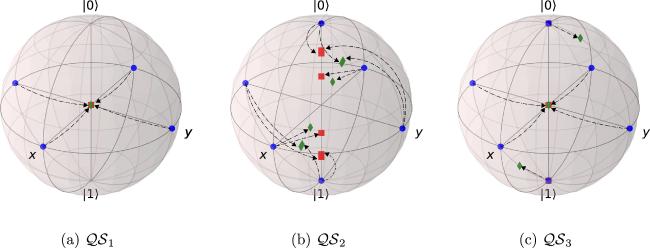
Figure 4. Illustration of optimal maskers. Panels (a)–(c) depict the transformation of the optimal maskers for different quantum sources, respectively. Blue points represent the input qubits, red squares represent the mixed states of subsystem B1 and green diamonds represent the mixed states of subsystem B2. Dotted arrows illustrate the correspondence between input and output qubits. |
Figure 4 intuitively demonstrates the transformation of the maskers on the input qubits. Blue points represent the input qubits (to be masked), red squares represent the mixed states of subsystem B1 and green diamonds represent the mixed states of subsystem B2. For ${ \mathcal Q }{{ \mathcal S }}_{1}$, the input qubits are uniformly situated on the equator of the Bloch sphere. Figure 4(a) shows that the output states of the masker are both situated at the origin, ensuring perfect information masking. For ${ \mathcal Q }{{ \mathcal S }}_{2}$, the input qubits are uniformly situated at the vertices of a regular octahedron. It has been proved that these qubits cannot be perfectly masked [23]. Figure 4(b) illustrates the one-to-one correspondence between the input and the output qubits. The primary difference between ${ \mathcal Q }{{ \mathcal S }}_{2}$ and ${ \mathcal Q }{{ \mathcal S }}_{3}$ lies in the probability distribution. Figure 4(c) shows that the optimal masker prioritizes masking these qubits with higher probabilities to the origin, thereby maximizing the extent to which quantum information is masked.
6. Conclusion
Designing optimal maskers is a prerequisite for the application of quantum masking in related quantum information processing tasks. This task belongs to optimal quantum state transformation [69]. In this paper, we present a variational quantum algorithm for designing QIM. This quantum–classical hybrid algorithm can be regarded as a quantum unsupervised learning. The loss value characterizes the performance of VQMs. If the loss value converges to zero, we obtain a perfect masker; otherwise, the perfect masker does not exist. However, we still obtain an optimal masker, which may still be useful in some situations.
To reduce state preparations and measurements, quantum parallelism is utilized to evaluate the loss function. Although we investigate the topic of quantum information masking, some techniques in this paper have the potential for wider applications such as the preparation of multipartite entanglement, and quantum secret sharing.
Finally, we point out that both empirical and theoretical results exhibit that the deployed ansatz heavily affects the performance of variational quantum algorithms, and VQMs are no exception. Research on designing ansatzes is underway [50]. Quantum information masking can provide specific research objects for the study on ansatzes.
Appendix A. SWAP test
Here, we provide some discussion on SWAP tests. The quantum circuit of a SWAP test is shown in figure 2. Suppose the input state is in the form of $\rho$ ⨂ σ. Calculation shows that the probabilities of obtaining 0 and 1 by measuring the first qubit are,A3 ) can be reformulated as,
$\begin{eqnarray}{p}_{0}=\frac{1}{2}(1+\mathrm{Tr}(\rho \sigma )),\end{eqnarray}$
$\begin{eqnarray}{p}_{1}=\displaystyle \frac{1}{2}(1-\mathrm{Tr}(\rho \sigma )).\end{eqnarray}$
Thus, the overlap between $\rho$ and σ can be obtained by subtraction, that is, $\begin{eqnarray}\mathrm{Tr}(\rho \sigma )={p}_{0}-{p}_{1}=\langle Z\rangle .\end{eqnarray}$
Let us regard the SWAP test as a function and denote it by ST( · ). Equation ( $\begin{eqnarray}\mathrm{Tr}(\rho \sigma )\equiv \mathrm{ST}(\rho \otimes \sigma ).\end{eqnarray}$
Note that measurement must be repeated enough times to evaluate $\mathrm{Tr}(\rho \sigma )$.In our main text, we need to obtain the evaluations of more complex quantities such as ${\sum }_{i=1}^{n}{p}_{i}\mathrm{Tr}({\rho }_{i}{\sigma }_{i})$. A trivial method is to evaluate each overlap $\mathrm{Tr}({\rho }_{i}{\sigma }_{i})$ and calculate the weighted mean. This method needs to repeat SWAP tests O(n) times. A better method that only runs the SWAP test once is as follows.
Our approach is to prepare a state in the form of ${\sum }_{i=1}^{n}{p}_{i}{\rho }_{i}\otimes {\sigma }_{i}$ and input it into the SWAP test. Due to the linearity of quantum circuits, the output state is in the form of,
$\begin{eqnarray}\begin{array}{l}| 0\rangle \langle 0| \otimes \displaystyle \frac{1}{4}\displaystyle \sum _{i}{p}_{i}\left[{\rho }_{i}\otimes {\sigma }_{i}+({\rho }_{i}\otimes {\sigma }_{i})S\right.\\ \quad \left.\,+S({\rho }_{i}\otimes {\sigma }_{i})+{\sigma }_{i}\otimes {\rho }_{i}\right]\\ \quad +\,| 1| \langle 1| \otimes \displaystyle \frac{1}{4}\displaystyle \sum _{i}{p}_{i}\left[{\rho }_{i}\otimes {\sigma }_{i}-({\rho }_{i}\otimes {\sigma }_{i})S\right.\\ \quad \left.\,-S({\rho }_{i}\otimes {\sigma }_{i})+{\sigma }_{i}\otimes {\rho }_{i}\right]\\ \quad +\,\cdots ,\end{array}\end{eqnarray}$
where S is the SWAP operator. Thus, the probabilities of obtaining 0 and 1 by measuring the first qubit are, $\begin{eqnarray}{p}_{0}=\displaystyle \frac{1}{2}+\displaystyle \frac{1}{2}\displaystyle \sum _{i}{p}_{i}\mathrm{Tr}({\rho }_{i}{\sigma }_{i}),\end{eqnarray}$
$\begin{eqnarray}{p}_{1}=\displaystyle \frac{1}{2}-\displaystyle \frac{1}{2}\displaystyle \sum _{i}{p}_{i}\mathrm{Tr}({\rho }_{i}{\sigma }_{i}).\end{eqnarray}$
Finally, we obtain the evaluation of ${\sum }_{i}{p}_{i}\mathrm{Tr}({\rho }_{i}{\sigma }_{i})$ by subtracting p0 and p1 as before. This indicates the linearity of ST( · ). We come to the following conclusions from the SWAP test:
1. If we input $\rho$ ⨂ σ, then it outputs $\mathrm{ST}(\rho \otimes \sigma )=\mathrm{Tr}(\rho \sigma );$
2. If we input ${\sum }_{i=1}^{n}{p}_{i}{\rho }_{i}\otimes {\sigma }_{i}$, then it outputs
$\begin{eqnarray}\mathrm{ST}(\displaystyle \sum _{i=1}^{n}{p}_{i}{\rho }_{i}\otimes {\sigma }_{i})=\displaystyle \sum _{i=1}^{n}{p}_{i}\mathrm{Tr}({\rho }_{i}{\sigma }_{i});\end{eqnarray}$
3. If we input ${\sum }_{i=1}^{n}{p}_{i}{\rho }_{i}\otimes {\sum }_{j=1}^{m}{p}_{j}{\sigma }_{j}$, then it outputs
$\begin{eqnarray}\mathrm{ST}(\displaystyle \sum _{i=1}^{n}{p}_{i}{\rho }_{i}\otimes \displaystyle \sum _{j=1}^{m}{p}_{j}{\sigma }_{j})=\displaystyle \sum _{i=1}^{n}\displaystyle \sum _{j=1}^{m}{p}_{i}{p}_{j}\mathrm{Tr}({\rho }_{i}{\sigma }_{j}).\end{eqnarray}$
Appendix B. Preparation of σ and $\tilde{\sigma }$
In our algorithms, a key step is to prepare σ and $\tilde{\sigma }$. Here, we introduce subroutines to prepare these states.
Suppose an arbitrary state ∣ψi⟩ ∈ S is generated by applying a known unitary operator Ui on the standard state ∣0⟩, that is,
$\begin{eqnarray}| {\psi }_{i}\rangle ={U}_{i}| 0\rangle .\end{eqnarray}$
Based on Ui, we construct a controlled unitary operator: $\begin{eqnarray}C\rm{-}U=\displaystyle \sum _{i=1}^{n}| i\rangle \langle i| \otimes {U}_{i},\end{eqnarray}$
where {∣i⟩} forms a set of orthonormal bases. C-U can be decomposed into n multi-qubit controlled operations [1].Given an initial state ${\sum }_{i=1}^{n}\sqrt{{p}_{i}}| i{\rangle }_{I}| 0{\rangle }_{A}$, by applying C-U on I and A, we obtain:
$\begin{eqnarray}| \psi \rangle =\displaystyle \sum _{i=1}^{n}\sqrt{{p}_{i}}| i{\rangle }_{I}| {\psi }_{i}{\rangle }_{A}.\end{eqnarray}$
In general, preparing an arbitrary state is difficult. However, efficient algorithms exist for the states to be of the form ${\sum }_{i=1}^{n}\sqrt{{p}_{i}}| i\rangle $. For example, Grover and Rudolph proposed a scheme that requires a linear number of operations regarding the number of qubits [70]. Applying M(θ) on ∣ψ⟩ gives us: $\begin{eqnarray}| {\rm{\Psi }}\rangle =\displaystyle \sum _{i}^{n}\sqrt{{p}_{i}}| i{\rangle }_{I}| {{\rm{\Psi }}}_{i}{\rangle }_{B}.\end{eqnarray}$
If we focus on the k subsystems marked by l, we obtain ${\sum }_{i}{p}_{i}{\sigma }_{i}^{{B}_{l}}$. Making another one and putting them together, we obtain ${\tilde{\sigma }}^{{B}_{l}}={\sum }_{i}{p}_{i}{\sigma }_{i}^{{B}_{l}}\otimes {\sum }_{j}{p}_{j}{\sigma }_{j}^{{B}_{l}}$.Note that our purpose is to prepare $\tilde{\sigma }={\left(\displaystyle \genfrac{}{}{0em}{}{N}{k}\right)}^{-1}{\sum }_{l}{\tilde{\sigma }}^{{B}_{{\boldsymbol{l}}}}$. To this end, let us associate l = {l1, l2, ⋯ ,l k} with an n-qubit quantum state defined as,
$\begin{eqnarray}| l\rangle =\cdots | 0{\rangle }_{{l}_{1}-1}| 1{\rangle }_{{l}_{1}}\cdots | 1{\rangle }_{{l}_{2}}\cdots | 1{\rangle }_{{l}_{k}}\cdots ,\end{eqnarray}$
that is the lith qubit is set at ∣1⟩ and the rest at ∣0⟩. For example, if l = {1, 3, 4} and N = 5, the corresponding state is ∣l⟩ = ∣1⟩1∣0⟩2∣1⟩3∣1⟩4∣0⟩5. Based on this, we introduce Dicke state $| {D}_{k}^{n}\rangle $ defined as, $\begin{eqnarray}| {D}_{k}^{N}\rangle ={\left(\displaystyle \genfrac{}{}{0em}{}{N}{k}\right)}^{-\tfrac{1}{2}}\displaystyle \sum _{l}| l\rangle ,\end{eqnarray}$
that is the equal superposition of all N-qubit states ∣l⟩ with Hamming weight k. Dicke states have garnered widespread attention for tasks in quantum information and as starting states for combinatorial optimization problems [71–74]. Then, we define the cyclic shift operation R[i,j] as below: $\begin{eqnarray}{R}_{[i,j]}| {x}_{i}{\rangle }_{i}| {x}_{i+1}{\rangle }_{i+1}\cdots | {x}_{j}{\rangle }_{j}=| {x}_{i+1}{\rangle }_{i}\cdots | {x}_{j}{\rangle }_{j-1}| {x}_{i}{\rangle }_{j},\end{eqnarray}$
which can be constructed by SWAP gates: $\begin{eqnarray}{R}_{[i,j]}=\displaystyle \prod _{r=0}^{j-i-1}S(j-r,j-r-1).\end{eqnarray}$
Based on R[i,j], the controlled cyclic shift operations can be constructed: $\begin{eqnarray}{C}_{0}\rm{-}{R}_{[i,j]}=| 0\rangle \langle 0| \otimes {R}_{[i,j]}+| 1\rangle \langle 1| \otimes I,\end{eqnarray}$
$\begin{eqnarray}{C}_{1}\rm{-}{R}_{[i,j]}=| 1\rangle \rangle 1| \otimes {R}_{[i,j]}+| 0\rangle \langle 0| \otimes I.\end{eqnarray}$
Next, we construct a controlled operation C-R defined as, $\begin{eqnarray}C\rm{-}R=\displaystyle \prod _{i=0}^{N-2}({C}_{1}^{N-i}{\rm{-}}{R}_{[1,N]}\cdot {C}_{0}^{N-i}{\rm{-}}{R}_{[\mathrm{1,1}+i]})\cdot {R}_{[1,N]},\end{eqnarray}$
where the superscript of C indicates the control qubit. The quantum circuit of C-R is shown in figure 5. Note that R[1,1] denotes identity operation. We reserve it here for clarity. It can be easily verified that C-R can determinedly shift target k subsystems into the last k subsystems according to ∣l⟩ encoded into the control qubits.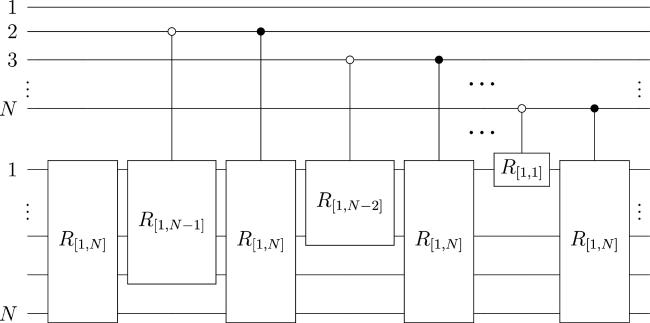
Figure 5. Diagram of quantum circuit for C-R. |
For example, if we input ∣l⟩∣$\Psi$i⟩, the last k subsystems of system B output the state ${\sigma }_{i}^{{B}_{l}}$.
Now, it is time to give the subroutine to prepare $\tilde{\sigma }$. We show the subroutine in algorithm 2 .
Algorithm 2.Prepare state $\tilde{\sigma }$
| Input: ${ \mathcal Q }{ \mathcal S }$, N, k, M |
| Output: $\tilde{\sigma }$ |
| 1 Prepare ${\sum }_{i=1}^{n}\sqrt{{p}_{i}}| i{\rangle }_{{I}_{1}}| {\psi }_{i}{\rangle }_{A}$; |
| 2 Apply M on systems A and R, where R refers to the necessary auxiliary system; |
| 3 Discard system I1, obtaining ${\sum }_{i=1}^{n}{p}_{i}| {{\rm{\Psi }}}_{i}{\rangle }_{B}\langle {{\rm{\Psi }}}_{i}{| }_{B}$; |
| 4 Repeat steps 1-3, obtaining another copy of ${\sum }_{j=1}^{n}{p}_{j}| {{\rm{\Psi }}}_{j}{\rangle }_{B^{\prime} }\langle {{\rm{\Psi }}}_{j}{| }_{B^{\prime} }$; |
| 5 Prepare Dicke state $| {D}_{k}^{N}{\rangle }_{{I}_{2}}$; |
| 6 Apply $C\rm{-}R$ on systems I2 and B; |
| 7 Apply $C\rm{-}R$ on systems I2 and $B^{\prime} $; |
| 8 Reserve systems ${B}_{N-k+1,N-k+2,\cdots ,N}$ and $B{{\prime} }_{N-k+1,N-k+2,\cdots ,N}$, obtaining $\tilde{\sigma }$; |
| 9 return $\tilde{\sigma }$. |
Similarly, σ can be prepared in a slightly different way and we show it in algorithm 3 .
Algorithm 3. Prepare state σ
| Input: ${ \mathcal Q }{ \mathcal S }$, N, k, M |
| Output: σ |
| 1 Prepare ${\sum }_{i=1}^{n}\sqrt{{p}_{i}}| i{\rangle }_{{I}_{1}}| {\psi }_{i}{\rangle }_{A}| {\psi }_{i}{\rangle }_{A^{\prime} }$; |
| 2 Apply M on systems A and R; |
| 3 Apply M on systems $A^{\prime} $ and $R^{\prime} $; |
| 4 Discard system I1, obtaining ${\sum }_{i=1}^{n}{p}_{i}| {{\rm{\Psi }}}_{i}{\rangle }_{B}\langle {{\rm{\Psi }}}_{i}{| }_{B}\otimes | {{\rm{\Psi }}}_{i}{\rangle }_{B^{\prime} }\langle {{\rm{\Psi }}}_{i}{| }_{B^{\prime} }$; |
| 5 Prepare Dicke state $| {D}_{k}^{N}{\rangle }_{{I}_{2}}$; |
| 6 Apply $C\rm{-}R$ on systems I2 and B; |
| 7 Apply $C\rm{-}R$ on systems I2 and $B^{\prime} $; |
| 8 Reserve systems ${B}_{N-k+1,N-k+2,\cdots ,N}$ and $B{{\prime} }_{N-k+1,N-k+2,\cdots ,N}$, obtaining σ; |
| 9 return σ. |
From algorithm 2 and 3 , it can be seen that the width of our algorithms is at most $3N+2\mathrm{log}n$. Suppose Ui are single-qubit unitary operations, it has been proved that an r-qubit controlled single-qubit unitary gate can be decomposed into a circuit with O(r2) single-qubit and CNOT gates [75]. Thus, C-U can be implemented using $O(n{\mathrm{log}}^{2}n)$ gates. In addition, the preparation of ${\sum }_{i=1}^{n}\sqrt{{p}_{i}}| i\rangle $ and $| {D}_{k}^{N}{\rangle }_{{I}_{3}}$ requires $O(\mathrm{log}n)$ and O(kN) gates, respectively [70, 76]. We further suppose VQM can be implemented with a polynomial number of operations. Then, the total number of gates of preparing $\tilde{\sigma }$ or σ is $O({poly}({kN},n{\mathrm{log}}^{2}n))$.