


1. Introduction
| 1. Introduction: This section presents the idea of fluid spheres with an expansion scalar and addresses modified gravity. It also contains prior information and emphasizes the significance of the study. | |
| 2. Mathematical framework: This section provides the fundamental mathematical foundation for the study. It contains the junction conditions, field equations, and energy-momentum tensor that serve as the study’s foundation. | |
| 3. Perturbation scheme and collapse equation: This section describes the perturbation scheme used in the analysis. We separate the static and non-static parts of modified field equations, mass functions, kinematical quantities, and conservation equations. Also, the dynamical collapse equation is derived in the same section, which helps to explain the behavior of fluid spheres. | |
| 4. Instability domains: In this section, we outline the methodology employed and examine the stability criteria for relativistic spheres at the N and PN epochs along with ${\mathbb{D}}$-dimensional modified correction terms via theoretical and pictorial representations. | |
| 5. Summary of work: The concluding part of the written work is found in this section along with some final observations on the significance and potential uses of the findings. | |
| 6. Intermediate mathematical terms (Appendix): It contains the comprehensive intermediate mathematics used in the deductions and evaluation procedures described in the text. This makes it possible for those who are interested to examine the computations while also ensuring that the technique is transparent. |
2. Mathematical framework
2.1. Fluid spheres, anisotropic matter tensor and some kinematic quantities
2.2. Theory and modified field equations
2.3. Mass function, Bianchi identities and matching conditions
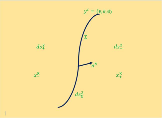
Figure 1. Pictorial representation hypersurface $({{ds}}_{{\rm{\Sigma }}}^{2})$ serves as the boundary separating the interior and exterior regions, denoted by ${{ds}}_{\pm }^{2}$, while normal to this hypersurface is a space-like unit vector nℵ and coordinates on the hypersurface and within the regions ${{ds}}_{\pm }^{2}$ are represented by yi and ${x}_{\pm }^{\aleph }$, respectively [22, 98, 101]. |
3. Perturbation method
3.1. Non-static configuration
3.2. Collapse equation
4. Instability domains
4.1. N and PN approximations
| • | The system will be in hydrostatic equilibrium if the gravitational forces $| \left({\mu }_{0}+{{\mathbb{P}}}_{r0}\right){\psi }_{1}^{{\prime} }\,-\tfrac{({\mathbb{D}}-2){\mu }_{0}r}{4{\psi }_{1}\alpha }\left({\psi }_{2}+\tfrac{2{\psi }_{3}}{r}\right)({{\mathbb{P}}}_{r0}-{\rm{\Lambda }})+2({{\mathbb{P}}}_{r0}-{{\mathbb{P}}}_{\perp 0}){\left(\tfrac{{\psi }_{3}}{r}\right)}^{{\prime} }| $ are balanced by the anti-gravitational and effective pressure forces $| {\left({{\mathbb{P}}}_{r0}\left({\psi }_{2}-\tfrac{2{\psi }_{3}}{r}\right)\right)}^{{\prime} }-\left(\tfrac{2}{r}({{\mathbb{P}}}_{r0}-{{\mathbb{P}}}_{\perp 0})+\tfrac{({\mathbb{D}}-2){\mu }_{0}r}{4{\psi }_{1}\alpha }{\rm{\Lambda }}\right)\left({\psi }_{2}+\tfrac{2{\psi }_{3}}{r}\right)| .$ |
| • | If the forces generated by $| \left({\mu }_{0}+{{\mathbb{P}}}_{r0}\right){\psi }_{1}^{{\prime} }\,-\tfrac{({\mathbb{D}}-2){\mu }_{0}r}{4{\psi }_{1}\alpha }\left({\psi }_{2}+\tfrac{2{\psi }_{3}}{r}\right)({{\mathbb{P}}}_{r0}-{\rm{\Lambda }})+2({{\mathbb{P}}}_{r0}-{{\mathbb{P}}}_{\perp 0}){\left(\tfrac{{\psi }_{3}}{r}\right)}^{{\prime} }| $ exceed those from $| {\left({{\mathbb{P}}}_{r0}\left({\psi }_{2}\,-\tfrac{2{\psi }_{3}}{r}\right)\right)}^{{\prime} }-\left(\tfrac{2}{r}({{\mathbb{P}}}_{r0}-{{\mathbb{P}}}_{\perp 0})+\tfrac{({\mathbb{D}}-2){\mu }_{0}r}{4{\psi }_{1}\alpha }{\rm{\Lambda }}\right)\left({\psi }_{2}+\tfrac{2{\psi }_{3}}{r}\right)| $, the system will achieve a stable state rather than collapsing, indicating that counter-gravitational forces and effective pressures satisfy the stability condition Γ > 1. |
| • | Conversely, if the contribution from $| \left({\mu }_{0}+{{\mathbb{P}}}_{r0}\right){\psi }_{1}^{{\prime} }\,-\tfrac{({\mathbb{D}}-2){\mu }_{0}r}{4{\psi }_{1}\alpha }\left({\psi }_{2}+\tfrac{2{\psi }_{3}}{r}\right)({{\mathbb{P}}}_{r0}-{\rm{\Lambda }})+2({{\mathbb{P}}}_{r0}-{{\mathbb{P}}}_{\perp 0}){\left(\tfrac{{\psi }_{3}}{r}\right)}^{{\prime} }| $ is less than the contribution from $| {\left({{\mathbb{P}}}_{r0}\left({\psi }_{2}-\tfrac{2{\psi }_{3}}{r}\right)\right)}^{{\prime} }-\left(\tfrac{2}{r}({{\mathbb{P}}}_{r0}-{{\mathbb{P}}}_{\perp 0})+\tfrac{({\mathbb{D}}-2){\mu }_{0}r}{4{\psi }_{1}\alpha }{\rm{\Lambda }}\right)\left({\psi }_{2}+\tfrac{2{\psi }_{3}}{r}\right)| $, the system will become unstable, with the adiabatic index Γ may fall within the open interval (0, 1). |
4.2. Graphical interpretation
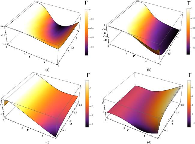
Figure 2. Pictorial representation for the dynamical behavior of non-static relativistic sphere models under the influence of ${\mathbb{D}}$-dimensional modified gravity at N epoch. |
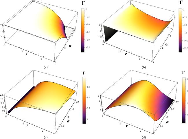
Figure 3. Diagrammatic representations of the spherically aligned relativistic sphere’s unstable and stable behavior over a range of values for different parameters at the PN era. |
| • | In figures 2(a) and (b), we used the Newtonian (N) framework. For figure 2(a), the parameters are ${\eta }_{i}^{,s}$, with values η1 = 0.4, η2 = 0.6, and η3 = 0.8, along with λ = 1.2 and Λ = 0.5. For figure 1(b), the parameters are ${\eta }_{i}^{,s}$, where η1 = 0.5, η2 = 0.8, and η3 = 1.1, with λ = 1.5 and Λ = 1.1. While some parameters remain consistent between figures 2(a) and (b), such as ${\mathbb{D}}=3$, n = 1.5, and the fixed range of α ∈ (0, 5) shown in both figures, the ranges of the adiabatic index Γ differ due to the varying parameter values used in each case. |
| • | In figures 3(a) and (b), we applied the PN framework. For figure 3(a), the parameters used are: ${\eta }_{i}^{,s}$, with specific values η1 = 0.5, η2 = 0.6, and η3 = 0.7, along with λ = 1.3, and Λ = 0.7. In figure 3(b), the parameters are ${\eta }_{i}^{,s}$, where η1 = 0.3, η2 = 0.8, and η3 = 1.1, with λ = 2.5, and Λ = 1.5. Although some parameters are consistent between figures 3(a) and (b), such as ${\mathbb{D}}=3$, n = 1.5, and the fixed range of α ∈ (0, 5) shown in both panels, the PN regime introduces additional parameters or corrections, like ${\mathbb{X}}$, ${\mathbb{Y}}$, and ${\mathbb{Z}}$, due to relativistic effects. This leads to variations in the range of the adiabatic index Γ, which differs as Γ ∈ (0, − 3) in figure 3(a) and Γ ∈ (0, − 12) in figure 3(b). |
| • | Next in the N domain, one observes from figure 2 stable and unstable regions for the specific sets of parameters, i.e., n = 3.5, λ = 1.35 Λ = 1.3, ${\mathbb{D}}=4$ and different values ${\eta }_{i}^{,s}$ for (c) and also different values ${\eta }_{i}^{,s}$, n = 5.5, λ = 1.45, Λ = 1.6 and ${\mathbb{D}}=5$ in (d) and the range of α ∈ (0, 2) in both panels (c) and (d) of figures 2. |
| • | We observe from figure 2 in the PN era, some stable and unstable regions for the specific sets of parameters, i.e., m0 = 1.5, n = 2.5, λ = 2.55, Λ = 1.2 ${\mathbb{D}}=4$ and different values ${\eta }_{i}^{,s}$ for (c) and also different values ${\eta }_{i}^{,s}$, with m0 = 2.0, n = 4.5, λ = 4.5, Λ = 1.4 and ${\mathbb{D}}=5$ in (d) and the range α is α ∈ (0, 2) in both panels (c) and (d) of figures 3. |
| • | Additionally, it is noted that in both scenarios, the adiabatic index ranges are marginally different. In these Figs, we find a relatively small stable zone in contrast to the unstable graphical representations. By taking into account the some specific choice of parametric values at N and PN eras, the figures 2 and 3 are obtained, which show the systematic graphical behavior of spherically symmetric compact system with ${\mathbb{D}}$-dimensional modified gravity theory. |
5. Summary of work
| • | It is important to note that the results in equations ( |
| • | Many of the additional curvature components introduced by ${\mathbb{D}}$-dimensional modified gravity in equations ( |
| • | We identified two key relations for the adiabatic index in equations ( |
| • | We established that when the system’s stiffness parameter equals the right-hand sides of relations ( |
| • | Consequently, the inequalities in equations ( |