


1. Introduction
The Bose–Einstein condensate (BEC), owing to its properties of coherence, superfluidity and macroscopic behavior, has stimulated the research interest of scientists in experimental and theoretical physics [1, 2]. The BEC has become important in various fields of physics, such as quantum communications [3], quantum computing [4] and quantum information [5]. The BEC is a unique system with macroscopic quantum characteristics [6], and extensive research has been conducted on the quantum dynamics of BECs in a double-well potential [7, 8]. Josephson tunneling of bosons has been detected in this double-well potential [9, 10]. Quantum tunneling is widely discussed because it is an important macroscopic quantum effect [11, 12]. It results in the oscillatory exchange of atoms between potential wells [13], akin to the Josephson effect in neutral atoms [14, 15]. There are weak interactions between the atoms in BECs, which lead to direct and alternating current phenomena, similar to the Josephson effect in superconductor systems in experiments [15–17].
The quantum state of a condensate system evolving with time can be solved using the adiabatic approximation. The adiabatic theorem is a fundamental concept in quantum theory, and is important for manipulating quantum states within quantum systems. Consequently, when investigating the dynamic behavior of BECs in soliton Josephson junctions (SJJs), a slow and stable adiabatic evolution method is typically necessary to prevent excitation of the BEC. Shortcuts to adiabaticity (STA) technology can expedite the adiabatic process while mitigating the impact of factors such as decoherence, noise and errors [18, 19]. Under ideal conditions, this technology can achieve the same stable results as the adiabatic process within a short time frame, offering effectiveness, feasibility and robustness. The implementation of STA technology encompasses various research approaches, including the quantum invariant-based inverse control method [20–22], variational approximation [23], the counter-diabatic driving algorithm [24, 25] and the transitionless quantum driving method [26–28]. These methods have been experimentally validated. This technology has been successfully applied in different fields such as photonics, atomic systems, quantum computing and cold atom systems in the realm of quantum systems [29–32].
The dynamic properties of atomic BECs have been widely explored and applied under the influence of a double-well potential [33–35]. In BEC theory, the interaction between BEC atoms can give rise to nonlinear characteristics [11]. Since a BEC is a macroscopic matter wave, it can form solitons. Khaykovich et al investigated the BEC of a dilute atomic gas of lithium atoms by modulating the interatomic nonlinear coefficients through the Feshbach resonance technique in reference [36]. However, for the SJJs system, even though solitons are one of the earliest nonlinear phenomena observed in nature [37–39], dynamical characterization remains an area for further exploration. It is well known that nonlinear system dynamics are complex, nonstationary, periodic systems, and nonlinear systems are sensitive to the initial conditions. In particular, small changes in the initial conditions in these systems can lead to large changes in the system. Superconducting Josephson junctions have been applied in highly sensitive magnetic measurements, quantum bit realizations, etc., but the SJJs studied in this paper also have promising applications in quantum precision measurements.
This article studies the BEC dynamics in an SJJs system with attractive interactions using the inverse control method of Lewis–Riesenfeld quantum invariants. Under the mean field approximation, the nonlinear Schrödinger equation is used to describe the wave function characteristics of the system model, and the Hamiltonian of the two-soliton system is mapped to the harmonic oscillator form. Next we study the relationship between the coupled time-containing Hamiltonian of the system and its corresponding invariant. Then we define the boundary conditions to realize the STA, and ultimately obtain a shortcut procedure for the tunneling rate between the double-well potential as a function of time. Thus we realize fast manipulation of the quantum state of the BEC dynamics in an SJJs system.
2. Model and basic equations
The SJJs system consists of two weakly coupled condensates with negative scattering lengths confined in a potential. This potential is composed of a three-dimensional harmonic confinement VH and a one-dimensional barrier Vdw. The harmonic trap is characterized by three-dimensional capture frequencies ωx, ωy and ωz, so ${V}_{{\rm{H}}}=({\omega }_{x}^{2}{x}^{2}+{\omega }_{y}^{2}{y}^{2}+{\omega }_{z}^{2}{z}^{2})/2$, and has been widely discussed in simplifying high-dimensional physical systems to low-dimensional physical models. Here, we transform the three-dimensional potential well to a two-dimensional space which consists of a horizontal coordinate x and radial direction r⊥. That is, ${V}_{{\rm{H}}}=\tfrac{1}{2}({\omega }_{x}^{2}{x}^{2}+{\omega }_{\perp }^{2}{r}_{\perp }^{2})$, where ${r}_{\perp }^{2}={y}^{2}+{z}^{2}$. So we can observe theoretically the state change of the BEC imprisoned in a double-well potential. On the other hand, Vdw divides the condensate into two parts that are weakly coupled due to particle tunneling through the potential barrier. It is interesting that we can obtain asymmetric potential wells by changing the position of the harmonic wells. In the model in this paper, the double potential well also has asymmetric properties. Tunneling between the two wells can affect the state of the BEC by changing the number of particles imprisoned in the potential wells. As shown in figure 1, we use the STA technique to set the tunneling rate to affect the two weakly coupled condensed states of the SJJs device, allowing fast manipulation of the quantum states.
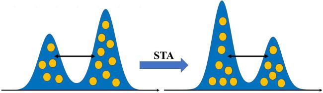
Figure 1. Diagram of the process for obtaining the target state t = tf from the initial state t = 0 of the coupled condensate by the STA technique. |
More explicitly, our model is a cigar-shaped condensate, so the capture potential energy in the x-direction is much weaker than in the radial direction r⊥ (ωx ≪ ω⊥) [40]. Under the two-mode approximation, the wave function of the system can be described as a coupling of the wave function in the horizontal coordinate x and radial directions
$\begin{eqnarray}\psi \left({r}_{\perp },x,t\right)={\phi }_{1}\left({r}_{\perp }-\displaystyle \frac{d}{2}\right){\psi }_{1}\left(x,t\right)+{\phi }_{2}\left({r}_{\perp }+\displaystyle \frac{d}{2}\right){\psi }_{2}\left(x,t\right),\end{eqnarray}$
where φ1,2 represents a wave function in the radial direction that is independent of time, ψ1,2 represents a time-dependent wave function in the x-direction and d represents the distance between the centers of two wave packets in the radial direction. In experiments dipole traps d are on the micrometer scale, and ψ1,2 meet the condition of the normalization ${\int }_{-\infty }^{\infty }({\left|{\psi }_{1}\right|}^{2}+{\left|{\psi }_{2}\right|}^{2}){\rm{d}}x=N$, where N represents the average total number of particles in the system. It is worth emphasizing that lithium condensed solitons with attractive interactions will exhibit instability and collapse when the atomic number exceeds a certain critical value Nc = 5 × 10³ [36]. In addition, one-dimensional bright solitons avoid collapsing at certain characteristic parameters.Since a strong capture potential is applied in the radial direction, φ1,2 fulfills the eigenvalue problem for a two-dimensional isotropic harmonic oscillator. It satisfies the harmonic oscillator ground state solution form $\exp \,(-{r}_{\perp }^{2}/2)$. In parallel, the time-dependent wave function of BEC dynamics in the x-direction satisfies one-dimensional Gross–Pitaevskii equations [40, 41]
$\begin{eqnarray}{\rm{i}}\displaystyle \frac{\partial {\psi }_{1}}{\partial t}=-\displaystyle \frac{1}{2}\displaystyle \frac{{\partial }^{2}{\psi }_{1}}{\partial {x}^{2}}-\mu | {\psi }_{1}{| }^{2}{\psi }_{1}+\displaystyle \frac{1}{2}{\nu }^{2}{x}^{2}{\psi }_{1}-\kappa {\psi }_{2},\end{eqnarray}$
$\begin{eqnarray}{\rm{i}}\displaystyle \frac{\partial {\psi }_{2}}{\partial t}=-\displaystyle \frac{1}{2}\displaystyle \frac{{\partial }^{2}{\psi }_{2}}{\partial {x}^{2}}-\mu | {\psi }_{2}{| }^{2}{\psi }_{2}+\displaystyle \frac{1}{2}{\nu }^{2}{x}^{2}{\psi }_{2}-\kappa {\psi }_{1}.\end{eqnarray}$
We normalize all spatial variables on ${a}_{\perp }=\sqrt{\left({\hslash }/m{\omega }_{\perp }\right)}$ and temporal ones on ${\omega }_{\perp }^{-1}$. So $\mu =2\pi \left|{a}_{\mathrm{sc}}\right|/{a}_{\perp }$ is the intensity of nonlinear interactions between atoms and asc denotes the condensate ground state transverse scattering length. Because we study attractive interactions between particles in the condensate model, here asc < 0; it can be adjusted through the Feshbach resonance method [42]. $\kappa \equiv \left|K\right|/{\omega }_{\perp }\gt 0$ represents the tunneling rate, which is a function of the coupling between the two wells. ν = ωx/ω⊥ is a trap asymmetry parameter. In the 7Li atom solitons we discuss ωx/2π = 70 Hz and ω⊥/2π = 700 Hz [43]. It is worth noting that a self-capturing state occurs when the initial asymmetry of the double-well potential reaches a certain critical value [44].
Under classical field theory, the classical Hamiltonian corresponding to equations (2 ) and (3 ) is expressed as
$\begin{eqnarray}\begin{array}{rcl}H & = & \displaystyle \int \displaystyle \sum _{j=1,2}\left(\displaystyle \frac{1}{2}{\left|\displaystyle \frac{\partial {\psi }_{j}}{\partial x}\right|}^{2}-\displaystyle \frac{\mu }{2}| {\psi }_{j}{| }^{4}+| {\psi }_{j}{| }^{2}{V}_{H}\left(x\right)\right){\rm{d}}x\\ & & -\displaystyle \int \kappa \left({\psi }_{1}^{* }{\psi }_{2}+{\psi }_{1}{\psi }_{2}^{* }\right){\rm{d}}x,\end{array}\end{eqnarray}$
where ${V}_{{\rm{H}}}=\tfrac{1}{2}{\nu }^{2}{x}^{2}$ represents a potential well in the x-direction.In the SJJs system, the BEC trapped in the double-well potential splits into two separate condensates when the potential barrier between the double-well potential is infinitely high, causing κ = 0. Additionally, when ν = 0 we can use the inverse scattering technique to obtain results for the existence of stationary normalized single-soliton solutions to equations (2 ) and (3 ) [41], denoted respectively as
$\begin{eqnarray}\begin{array}{rcl}{\psi }_{1} & = & \displaystyle \frac{{N}_{1}\sqrt{\mu }}{2}{\rm{sech}} \left[\displaystyle \frac{\mu {N}_{1}x}{2}\right]{{\rm{e}}}^{{\rm{i}}{\theta }_{1}},\\ {\psi }_{2} & = & \displaystyle \frac{{N}_{2}\sqrt{\mu }}{2}{\rm{sech}} \left[\displaystyle \frac{\mu {N}_{2}x}{2}\right]{{\rm{e}}}^{{\rm{i}}{\theta }_{2}}.\end{array}\end{eqnarray}$
We take equation (5 ) as the initial state and bring it into equation (4 ). Omitting the energy term proportional to N, we can obtain the effective classical Hamiltonian quantity for representing a two-soliton system as
$\begin{eqnarray}{H}_{\mathrm{SJJ}}=-\displaystyle \frac{{\mu }^{2}}{24}\left({N}_{1}^{3}+{N}_{2}^{3}\right)-\displaystyle \frac{4\kappa {N}_{1}{N}_{2}}{N}I\left(z\right)\cos \theta .\end{eqnarray}$
Here N1 + N2 = N, N1,2 represent the number of particles captured by a double-well potential, z = (N2 − N1)/N is the normalized population imbalance, which represents the dynamic change of particle number, and phase θ = θ2 − θ1 is the phase difference. Moreover, $I(z)={\int }_{0}^{\infty }{\left({\cosh }^{2}\left(\theta \right)+{\sinh }^{2}\left({zx}\right)\right)}^{-1}\approx 1-0.21{z}^{2}$. Here we also omit the constant energy term that is proportional to N.Consequentially, we replace N1,2 in equation (6 ) with z. The effective classical Hamiltonian of the SJJs system can be transformed into a function with z and θ as independent variables
$\begin{eqnarray}{H}_{\mathrm{SJJ}}=\kappa N\left(-\displaystyle \frac{{\rm{\Lambda }}}{2}{z}^{2}-(1-0.21{z}^{2})(1-{z}^{2})\cos \theta \right),\end{eqnarray}$
where ${\rm{\Lambda }}=\tfrac{{\mu }^{2}{N}^{2}}{16\kappa }=\tfrac{{\mu }^{2}{N}^{2}{\omega }_{\perp }}{16| K| }=\tfrac{\alpha }{\kappa }$ is the effective nonlinear parameter.The equations $\dot{\theta }=-\partial {H}_{\mathrm{SJJ}}/\partial z$ and $\dot{z}=\partial {H}_{\mathrm{SJJ}}/\partial \theta $ for canonical variables z and θ can be obtained with the Hamiltonian equation (7 ) as
$\begin{eqnarray}\begin{array}{rcl}\dot{\theta } & = & {\rm{\Lambda }}z-2z(1.21-0.42{z}^{2})\cos \theta ,\\ \dot{z} & = & (1-{z}^{2})(1-0.21{z}^{2})\sin \theta ,\end{array}\end{eqnarray}$
where the dots denote derivatives with respect to effective (dimensionless) time τ = κNt.As shown in figure 2, in order to obtain the dynamics of equation (8 ), we discuss two initial conditions on the phase difference for the existence of a steady-state solution, θ(0) = π, $z=\pm \sqrt{1.21/0.42+{\rm{\Lambda }}/0.84}$ and θ(0) = 0, $z\,=\pm \sqrt{1.21/0.42-{\rm{\Lambda }}/0.84}$. We find that the parameter Λ affects the amplitude and period of the Josephson oscillation. In particular, the asymmetric oscillations of z(t) when Λ crosses a critical value imply that the system undergoes a macroscopic self-capture effect in figure 2(b).
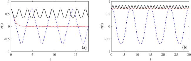
Figure 2. Plot of population imbalance z(t) versus dimensionless time with the initial condition z(0) = 0.7: (a) θ(0) = π, Λ = 5 (blue dashed line), Λc = 5.9608 (red dotted line), Λ = 7 (black solid line); (b) θ(0) = 0, Λ = 1 (blue dashed line), Λc = 2.0084 (red dotted line), Λ = 7 (black solid line). |
3. Fast shortcut to adiabatic evolution
The population imbalance term in equation (7 ) is very important, reflecting the difference between the dynamics of the SJJs system. Λ is particularly important in this term and we would like to change Λ more easily. In particular, under the condition of certain μN, we use the STA technique to change the control parameter κ for the purpose of manipulating Λ.
In the following, we use the Taylor expansion formula $\sqrt{1-{z}^{2}}\approx 1-{z}^{2}/2$, and $\cos \theta \approx 1-{\theta }^{2}/2$ causes the effective potential energy to remove the dependence on z. We omit the higher-order quantity and the constant energy term to change the Hamiltonian expression of the SJJs system into
$\begin{eqnarray}{H}_{\mathrm{STA}}=\displaystyle \frac{\kappa (t)N}{2}\left(2.42-{\rm{\Lambda }}\right){z}^{2}+\displaystyle \frac{1}{2}\kappa (t)N{\theta }^{2}.\end{eqnarray}$
We provide an expression for the Hamiltonian quantity in the atomic bosonic Josephson junctions (BJJs) system in the appendix , which visually express the difference between the SJJs and BJJs systems when Λ ≠ 0. From equations (9 ) and (A2 ) the difference in the soliton population imbalance can be seen, which leads to a difference in the properties of the SJJs system. We find that the nonlinear effect disappears as z tends to zero; at this point the properties of SJJs and BJJs system dynamics are almost identical.
When studying the dynamics of the system corresponding to equation (9 ) its quantum states are more difficult to find during evolution. We utilize a method based on Lewis–Riesenfeld invariant inverse control to accelerate the evolution of the system state. The Lewis–Riesenfeld method with time-invariance theory [45, 46] shows that the invariant I(t) satisfies the following equation:
$\begin{eqnarray}\displaystyle \frac{{\rm{d}}I}{{\rm{d}}t}=\displaystyle \frac{\partial I}{\partial t}+\displaystyle \frac{1}{{\rm{i}}{h}}[I,{H}_{\mathrm{STA}}]=0.\end{eqnarray}$
From equations (9 ) and (10 ), we obtain an expression for the invariant corresponding to the SJJs model as
$\begin{eqnarray}\begin{array}{l}I=\displaystyle \frac{1}{2}\left\{{\left(\displaystyle \frac{\theta }{\rho }A{\left(t\right)}^{-\tfrac{1}{2}}\right)}^{2}{{\rm{\Omega }}}_{0}^{2}+\left[\Space{0ex}{3.25ex}{0ex}2\rho A{\left(t\right)}^{\displaystyle \frac{1}{2}}z\right.\right.\\ \,\left.{\left.-\,\left(\dot{\rho }+\displaystyle \frac{\rho \dot{A}\left(t\right)}{2A\left(t\right)}\right)A{\left(t\right)}^{-\tfrac{1}{2}}\theta \right]}^{2}\right\},\end{array}\end{eqnarray}$
where we set A(t) = N(2.42κ(t) − α)/2.Meanwhile we find that auxiliary parameters $\rho$(t) satisfies the following Ermakov equation:
$\begin{eqnarray}\ddot{\rho }+{\rm{\Omega }}{\left(t\right)}^{2}\rho =\displaystyle \frac{{{\rm{\Omega }}}_{0}^{2}}{{\rho }^{3}},\end{eqnarray}$
where the dots represent time derivatives. The Ermakov equation shows that I(t) obeys HSTA(t) [20]. α0 = α(0) and ${\rm{\Omega }}{\left(t\right)}^{2}$ can be defined as $\begin{eqnarray}\begin{array}{l}{\rm{\Omega }}{\left(t\right)}^{2}=\kappa {\left(t\right)}^{2}{N}^{2}\left(2.42-{\rm{\Lambda }}\right)-\displaystyle \frac{\dot{\kappa }{\left(t\right)}^{2}}{4\kappa {\left(t\right)}^{2}{\left(2.42-{\rm{\Lambda }}\right)}^{2}}\\ \,+\,\displaystyle \frac{\ddot{\kappa }\left(t\right)\kappa \left(t\right)(2.42-{\rm{\Lambda }})-\dot{\kappa }{\left(t\right)}^{2}}{2\kappa \left(t\right)\left(2.42-{\rm{\Lambda }}\right)}.\end{array}\end{eqnarray}$
To achieve the effect of STA, the intermediate evolution process does not need to be controlled precisely [35]. At the first and last moments, the system is in the eigenstate of the invariant I while it is also in the eigenstate of H. That is, H and I satisfy the commute relation at the first and last moments, and both share the set of eigenstates. The initial and final moments of the invariant satisfy the relationship equation
$\begin{eqnarray}\left[I\left(0\right),{H}_{\mathrm{STA}}\left(0\right)\right]=0,\qquad \left[I\left({t}_{f}\right),{H}_{\mathrm{STA}}\left({t}_{f}\right)\right]=0.\end{eqnarray}$
Through equation (14 ), we can obtain the six frictionless boundary conditions for the auxiliary parameter $\rho$, expressed as
$\begin{eqnarray}\begin{array}{rcl}\rho \left(0\right) & = & 1,\qquad \rho \left({t}_{f}\right)={r}_{1},\\ \dot{\rho }\left(0\right) & = & {\ddot{\rho }}_{1}\left(0\right)=\dot{\rho }\left({t}_{f}\right)=\ddot{\rho }\left({t}_{f}\right)=0,\end{array}\end{eqnarray}$
where $r=\sqrt{{{\rm{\Omega }}}_{0}/{\rm{\Omega }}({t}_{f})}$.Boundary conditions determine the form of scale factors that can be considered in inverse engineering. The initial and final states of the observing system are determined by the boundary conditions, which construct the initial and final structures of the invariant. We apply the polynomial $\rho (t)={\sum }_{j=0}^{5}{a}_{j}{s}^{j}$ from reference [24] with s = t/tf. We obtain the polynomial expression for $\rho$ by calculating the above boundary conditions
$\begin{eqnarray}\rho \left(t\right)=1+\left(10{s}^{3}-15{s}^{4}+6{s}^{5}\right)\left(r-1\right).\end{eqnarray}$
The STA protocol corresponding to κ(t) in equation (9 ) obeys the α(t) modulation in equation (12 ). Here we use equations (12 ) and (13 ) to obtain the expression for the tunneling rate as
$\begin{eqnarray}\ddot{\kappa }=\displaystyle \frac{4{A}^{2}(t)\left[\tfrac{2A(0)\kappa (0)N}{{\rho }^{4}(t)}-\tfrac{\ddot{\rho }(t)}{\rho (t)}\right]+3{\dot{A}}^{2}(t)-8{A}^{3}(t)\kappa (t)N}{2.42{NA}(t)}.\end{eqnarray}$
From equations (16 ) and (17 ), we can obtain the evolutionary trajectory of the tunneling rate for the STA design. In the appendix we give an extension of the shortcut technique for the tunneling rate in the BJJs system.
4. Stability analysis of the shortcut protocol
We find that μ hardly affects the application of the STA technique in the SJJs system. On the other hand, the STA technique does not work when μ decreases to a certain value in the BJJs system. Thus we chose the ground state wave function at the interatomic interaction strength μ ∼ 10, which is closer to the SJJs system we studied. The Gaussian functional form is used to describe the ground state wave function of the BJJs system when μ = 1 [38]. Figure 3 shows the adiabatic evolution of the system tunneling rate. We compare the shortcut protocol that uses a polynomial ansatz for $\rho$(t) with a linear rise: $\kappa (t)=\exp (-0.0693t/{t}_{f})$. For the initial end state of the system, we fix the initial value of the tunneling rate to κ(0) = 1 and the value of the ending moment to κ(tf) = 0.5 [47]. Here the total number of particles N = 100. The value of Λ varies between 0.0625 and 0.125, which is less than the Λc shown in figure 2. There are Josephson oscillations in the system. This means that the system shows the Josephson oscillation phenomenon. We can see that the tunneling rate of the SJJs system is different from that of linear evolution.
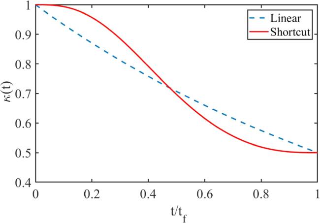
Figure 3. Adiabatic evolution of the tunneling rate with time plotted for the SJJs system: shortcut protocol (red solid line) tf = 1, and linear ramping (blue dashed line) tf = 10. Other parameters: N = 100, κ(0) = 1, κ(tf) = 0.5. |
Figure 4 demonstrates the variation of tunneling rate in the SJJs and BJJs systems under different adiabatic shortcut evolution time conditions. We set the initial and target values of the tunneling rate κ(0) = 0.0001 and κ(tf) = 0.001 [47, 48], which means that the value of Λ is larger than its critical value and there is self-trapping behavior in the system. In figure 4(a), when the evolution time tf = 5, 0.2, 0.05 in the SJJs system, the tunneling rate evolution trajectories are closer. However, under the same conditions in the BJJs system, the fluctuation range of the tunneling rate becomes larger, as shown in figure 4(b). In a word, when tf is small enough, the average value of the tunneling rate will become larger during evolution. Comparing figures 4(a) and (b), we can observe that the SJJs system is more stable, especially over a short time to realize the adiabatic shortcut technique. Therefore, under the same conditions, we can manipulate the quantum states of the SJJs system more easily.
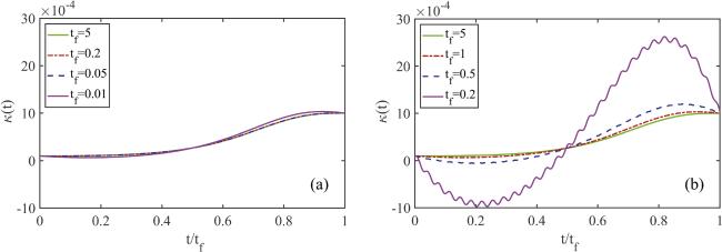
Figure 4. Evolution of κ(t) for polynomial shortcut protocols for different final times: (a) in the SJJs system, tf = 5, 0.2, 0.05, 0.01; (b) in the BJJs system, tf = 5, 1, 0.5, 0.2. Other parameters: κ(0) = 0.0001, κ(tf) = 0.001 and N = 100. |
Moreover, when we use the shortcut tool technique to modulate the tunneling rate in the SJJs system to tf < 0.006, the tunneling rate shows some negative values. For the BJJs system, the tunneling rate will be negative below a threshold of tf = 0.6. This is because the destruction of the adiabatic environment leads to the failure of modulation of the STA technique. These thresholds demonstrate the better robustness of the SJJs system under the same conditions.
In the following, we use the split-step Fourier method (a numerical calculation method) to solve equations (2 ) and (3 ) with STA-designed tunneling coefficients. We obtain the evolution of the wave function at the moments t = 0 and tf = 1. Figures 5(a)–(d) correspond to initial population imbalances z(0) = 0, z(0) = 0.2, z(0) = 0.6 and z(0) = 0.98, respectively. Nevertheless, we find that the tunneling effect has no effect on the wave function of the SJJs system because the system’s effective nonlinear parameter term fails when z(0) = 0, as shown in figure 5(a). Figures 5(b)–(d) indicate the presence of the Josephson oscillation phenomenon. When κ changes N1 and N2, the peaks and widths of the two wave function densities undergo opposite changes. As z(0) becomes larger, the amplitude of the oscillation becomes larger. κ(t) has an effect on the Josephson oscillation period. This is manifested in the reduction of κ(t), leading to smaller oscillation periods. Figure 6 shows the evolution of the different initial states to the corresponding end states during the evolution time tf = 1, which corresponds to figure 5.
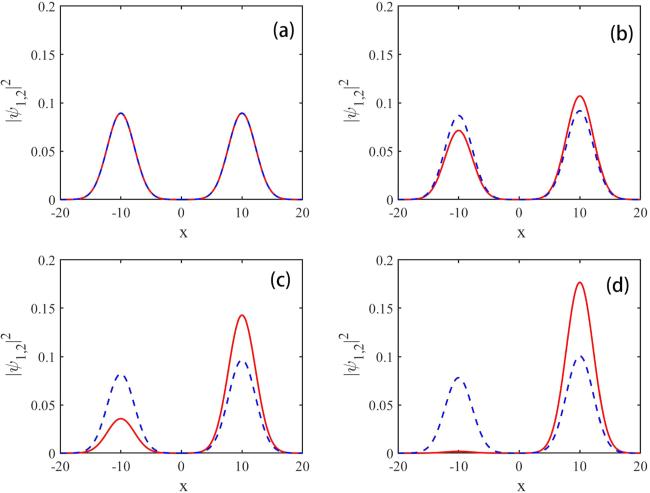
Figure 5. The density distribution of the two-component wave function ${\left|{\psi }_{\mathrm{1,2}}\right|}^{2}$ in the x-direction for different values of z (initial state shown by the solid red line and end state shown by the dashed blue line): (a) z(0) = 0, (b) z(0) = 0.2, (c) z(0) = 0.6, (d) z(0) = 0.98. Other parameters: κ(0) = 1, κ(tf) = 0.5, tf = 1, μ = 0.1 and N = 10. |
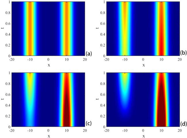
Figure 6. The propagation contour map of wave packets ${\left|{\psi }_{\mathrm{1,2}}\right|}^{2}$ in the process of fast transport designed by the inverse engineering method at z = 0, 0.2, 0.6 and 0.98. Parameters are the same as in figure 5. |
In order to get the change in the effective nonlinear parameter Λ of the SJJs system, we use the evolution of the polynomial shortcut technique to set the tunneling rate κ(t). The value of Λ varies from 0.0625 to 0.125, smaller than the condition of the critical value of 2.0084 shown in figure 2. The system will not experience self-trapping effects when Λ is less than the critical condition [44]. So when z(0) is not equal to zero, the system will undergo Josephson oscillatory behavior.
Finally, we discuss the effectiveness of shortcut protocols. Since κ(t) ≠ 0, we use the Gaussian form as the reference state, as proved in reference [41]
$\begin{eqnarray}{\widetilde{\psi }}_{j}=\displaystyle \frac{{\nu }^{\tfrac{1}{4}}\sqrt{{N}_{j}({t}_{f})}}{{\pi }^{\tfrac{1}{4}}}{{\rm{e}}}^{-\nu {x}^{2}/2}{{\rm{e}}}^{{\rm{i}}{\theta }_{j}}.\end{eqnarray}$
N is constant during the oscillation period and the two wave functions satisfy ${\int }_{-\infty }^{\infty }({\left|{\psi }_{1}\right|}^{2}+{\left|{\psi }_{2}\right|}^{2}){\rm{d}}x=N$. In figure 7, we use overlap to characterize the fidelity
$\begin{eqnarray}F={\left|\,{,}\left\langle {\psi }_{1}(x,{t}_{f})| {\widetilde{\psi }}_{1}(x,{t}_{f})\right\rangle \,\right|}^{2}+{\left|\,{,}\left\langle {\psi }_{2}(x,{t}_{f})| {\widetilde{\psi }}_{2}(x,{t}_{f})\right\rangle \,\right|}^{2},\end{eqnarray}$
where ψ1,2(x, tf) represents the target state at t = tf obtained through inverse engineering. At the same time we calculate the area overlap differences of the wave function density to verify that the above fidelity solution is correct and usable.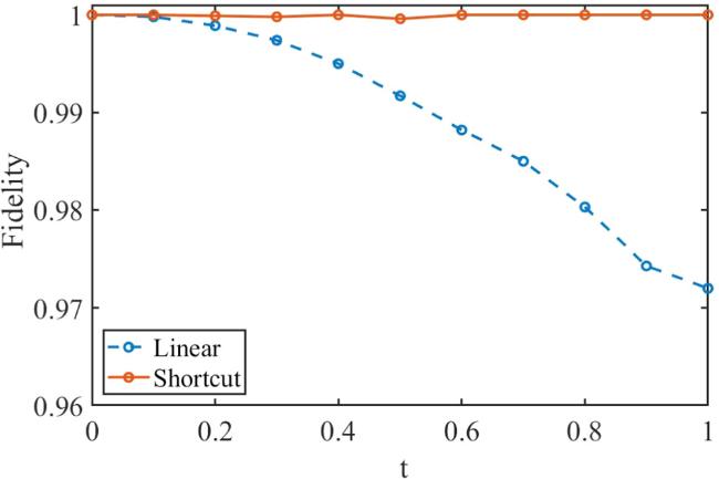
Figure 7. Fidelity versus evolution time for the linear ramping reference (blue dashed line) and the STA protocol (orange solid line). The parameters are the same as in figure 5. |
To achieve the manipulated evolution from κ(0) = 1 to κ(tf) = 0.5, we set the linear ramping evolution to take a longer time tf = 10, while the STA technique only takes tf = 1. We calculate the fidelity of the shortcut protocol and linear ramping with z(0) = 0.98, respectively. The number of particles exhibits a sinusoidal-like variation during this evolution, which is consistent with the evolution of the number of layouts over time in figure 2. Meanwhile, we can clearly understand that the STA technique is perfectly suitable for our system, and the fidelity of both the initial and end states is close to 1. However, the fidelity of the end state of the linear equation is about 0.9720, which is comparatively lower than the design of the shortcut protocol.
5. Higher-order solutions of auxiliary functions
We analyze the stability of the shortcut protocol in figure 4, and we find that the system is adversely affected by the sloshing amplitude [49, 50]. The duration of the adiabatic shortcut protocol modulation process is short, presenting a more pronounced waveform in figure 4(b). The results show that the SJJs system is less affected by the sloshing amplitude and has strong robustness. In order to address the detrimental effects of the sloshing amplitude, we use a higher-order polynomial solution of the auxiliary equations to minimize the effect of the sloshing amplitude in the model.
The solution process of the higher-order equation is similar to equation (16 ), which requires more boundary conditions. In order to obtain the third-order boundary conditions for the auxiliary function, we perform the derivation of equation (12 ), which is expressed as
$\begin{eqnarray}\dddot{\rho }(t)+2{\rm{\Omega }}(t)\dot{{\rm{\Omega }}}(t)\rho (t)+{{\rm{\Omega }}}^{2}(t)\dot{\rho }(t)=-3{{\rm{\Omega }}}_{0}^{2}\rho {\left(t\right)}^{-4}\dot{\rho }(t).\end{eqnarray}$
From equation (15 ), we know that $\dot{{\rm{\Omega }}}(t)=0$, $\dot{\rho }(t)=0$ when t = 0 and t = tf, so we can get
$\begin{eqnarray}\dddot{\rho }(0)=\dddot{\rho }({t}_{f})=0.\end{eqnarray}$
In order to meet the eight boundary conditions of equations (15 ) and (21 ), we use a polynomial trajectory of order seven for $\rho (t)={\sum }_{j=0}^{7}{a}_{j}{s}^{j}$, written in normalized time as
$\begin{eqnarray}\rho \left(t\right)=1+\left(r-1\right)\left(35{s}^{4}-84{s}^{5}+70{s}^{6}-20{s}^{7}\right).\end{eqnarray}$
Comparing equations (16 ) and (22 ), we find that the auxiliary equation with j = 7 approaches the end state faster than j = 5. This increases the robustness of the shortcut method.
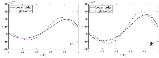
We can obtain a graph of the tunneling rate with time, shown in figure 8. It can be clearly seen that the seventh-order equation reduces the effect from the sloshing amplitude. As a result, the evolution curves of the SJJs and BJJs systems become flatter and the experimental results become more stable under the same conditions.
Figure 8. (a) Evolution of κ(t) required for two polynomial shortcut protocols in SJJs systems and N = 5. (b) Evolution of κ(t) required for two polynomial shortcut protocols in BJJs systems, N = 30 (red line). In all simulations κ(0) = 0.0001, κ(tf) = 0.001 and tf = 1. |
6. Conclusion
In conclusion, we have investigated the dynamics of BECs in the SJJs system through the STA technique. These are then analyzed and compared with the BJJs system. It is shown that STA exhibits greater operability and robustness in the SJJs system. In this paper, we map the Hamiltonian of the SJJs and BJJs systems onto time-containing harmonic-like oscillators, showing that the invariant-based inverse control method has great application prospects. We obtain the evolutionary trajectories of the tunneling rate by inverse engineering and realize precise control of the quantum states in the SJJs and BJJs systems. We demonstrate that the SJJs system can achieve modulation of the tunneling rate corresponding to ordinary adiabatic evolution within a very short adiabatic shortcut evolution time (tf > 0.006). In addition, we use higher-order expression of the polynomials; this can reduce the detrimental effects of the sloshing amplitude that appear in the lower-order evolution curves. Thus we can improve the stability of the experimental results. The greater stability exhibited by the SJJs system will contribute to the preparation of states and research in quantum metrology. At the same time, it also provides some theoretical support for the application of SJJs in quantum precision measurement. Thus, STA has important advantages for realizing future experiments on SJJs.
Acknowledgments
This work was supported by the National Natural Science Foundation of China (Grant nos. 12075145 and 12211540002) and the Science and Technology Commission of Shanghai Municipal (Grant no. 2019SHZDZX01-ZX04).
Appendix.Shortcut equation for the BJJs system
The BJJs model is similar to the SJJs model in that the BJJs system is obtained by constructing a BEC in a double-well potential. In the BJJs system, we assume that the wave function corresponding to the boson takes the form of an independent Gaussian solution and is denoted as
$\begin{eqnarray}{\psi }_{j}=\displaystyle \frac{{\nu }^{\tfrac{1}{4}}\sqrt{{N}_{j}}}{{\pi }^{\tfrac{1}{4}}}{{\rm{e}}}^{-\nu {x}^{2}/2}{{\rm{e}}}^{{\rm{i}}{\theta }_{j}}.\end{eqnarray}$
Taking z and θ as variables, we write the expression for the BJJs effective classical Hamiltonian as
$\begin{eqnarray}{H}_{\mathrm{BJJ}}=\displaystyle \frac{\kappa N}{2}\left(1-\lambda \right){z}^{2}+\displaystyle \frac{1}{2}\kappa N{\theta }^{2},\end{eqnarray}$
where $\lambda =\tfrac{\sqrt{\nu }\mu N}{2\sqrt{2\pi }\kappa }=\tfrac{\sqrt{\nu }\mu N{\omega }_{\perp }}{2\sqrt{2\pi }| K| }=\tfrac{\beta }{\kappa }$ is the effective nonlinearity parameter of the BJJs system.Similarly, through the Lewis–Riesenfeld with time-invariant theory method [45, 46], we get the expression for the BJJs system invariant as
$\begin{eqnarray}\begin{array}{l}{I}_{\mathrm{BJJ}}=\displaystyle \frac{1}{2}\left\{{\left(\displaystyle \frac{\theta }{b}C{\left(t\right)}^{-\tfrac{1}{2}}\right)}^{2}{{\rm{\Omega }}}_{0}^{2}+\left[\Space{0ex}{3.25ex}{0ex}2{bC}{\left(t\right)}^{\displaystyle \frac{1}{2}}z\right.\right.\\ \,\left.{\left.-\,\left(\dot{b}+\displaystyle \frac{b\dot{C}\left(t\right)}{2C\left(t\right)}\right)C{\left(t\right)}^{-\tfrac{1}{2}}\theta \right]}^{2}\right\},\end{array}\end{eqnarray}$
where C(t) = N(κ(t) − β)/2.b(t) satisfies the Ermakov equation expressed as
$\begin{eqnarray}\ddot{b}+\omega {\left(t\right)}^{2}b=\displaystyle \frac{{\omega }_{0}^{2}}{{b}^{3}},\end{eqnarray}$
where $\begin{eqnarray}\begin{array}{l}\omega {\left(t\right)}^{2}=\kappa {\left(t\right)}^{2}{N}^{2}\left(1-\lambda \right)-\displaystyle \frac{\dot{\kappa }{\left(t\right)}^{2}}{4\kappa {\left(t\right)}^{2}{\left(1-\lambda \right)}^{2}}\\ \,+\,\displaystyle \frac{\ddot{\kappa }\left(t\right)\kappa \left(t\right)(1-\lambda )-\dot{\kappa }{\left(t\right)}^{2}}{2\kappa \left(t\right)\left(1-\lambda \right)}.\end{array}\end{eqnarray}$
b(t) must satisfy the boundary conditions
$\begin{eqnarray}\begin{array}{rcl}b\left(0\right) & = & 1,\qquad b\left({t}_{f}\right)={r}_{\mathrm{BJJ}},\\ \dot{b}\left(0\right) & = & \ddot{b}\left(0\right)=\dot{b}\left({t}_{f}\right)=\ddot{b}\left({t}_{f}\right)=0,\end{array}\end{eqnarray}$
where ${r}_{\mathrm{BJJ}}=\sqrt{{\omega }_{0}/\omega ({t}_{f})}$ .Based on the polynomial expression, we get the fifth-degree polynomial of the auxiliary equation with respect to time in the BJJs system as
$\begin{eqnarray}b\left(t\right)=1+\left(10{s}^{3}-15{s}^{4}+6{s}^{5}\right)\left({r}_{\mathrm{BJJ}}-1\right).\end{eqnarray}$
The third-order boundary conditions for the auxiliary equations of the system are
$\begin{eqnarray}\dddot{b}(0)=\dddot{b}({t}_{f})=0.\end{eqnarray}$
In equation (A6 ), through the auxiliary function and its the first- and second-order boundary equations, the joint equation (A8 ) gives the seventh-order expression for the auxiliary equation as
$\begin{eqnarray}b\left(t\right)=1+\left({r}_{\mathrm{BJJ}}-1\right)\left(35{s}^{4}-84{s}^{5}+70{s}^{6}-20{s}^{7}\right).\end{eqnarray}$
The tunneling rate is obtained as
$\begin{eqnarray}\ddot{\kappa }=\displaystyle \frac{4{C}^{2}(t)\left[\tfrac{2C(0)\kappa (0)N}{{b}^{4}(t)}-\tfrac{\ddot{b}(t)}{b(t)}\right]+3{\dot{C}}^{2}(t)-8{C}^{3}(t)\kappa (t)N}{{NC}(t)}.\end{eqnarray}$