


1. Introduction
Rogue waves are unique solutions of partial differential equations in the form of high-amplitude bumps in a plane wave background [1–3]. Such a solution is only a particular case of a much more general class of periodic structure. The latter are multi-parameter families of solutions that may take a variety of forms and configurations [4]. One example is the family of doubly periodic solutions of the nonlinear Schrödinger equation (NLSE). This is the fundamental (first order) multi-parameter family of solutions that are periodic both in space and in time [5]. The doubly periodic solutions involve several important subsets such as Akhmediev breathers [6], Kuznetsov-Ma solitons (KMS) [7, 8], and their limiting case with an infinite period—Peregrine rogue waves [9]. These solutions are related to the focusing case of the NLSE. The richness of their mathematical structure leads to many physical phenomena hidden within the family of solutions. In particular, these solutions describe the phenomenon of modulation instability [6, 10–12] known since the 1960s. These solutions also allow us to explain the well-known paradox of Fermi–Pasta–Ulam recurrence [13–16]. Rogue wave events are also found to be within this family [17]. Among the most complicated physical phenomena that can be explained in terms of exact solutions of the NLSE are integrable turbulence [18] and supercontinuum generation [19, 20].
The NLSE with focusing nonlinearity is not the only equation that admits the family of doubly periodic solutions. The case of a defocusing NLSE is no less intriguing [21]. However, the family of double periodic solutions in the defocusing case describes different sets of physical phenomena. They are related to multiple interactions and collision of dark solitons [21].
Periodic solutions of partial differential equations are also known as breathers. One of the physical processes that can lead to scalar breathers is the nonlinear interaction of fundamental solitons. This type of solution is known as higher-order solitons or Satsuma–Yajima breathers [22]. They involve two or more eigenvalues of the inverse scattering transform. Generally, the eigenvalues in the higher-order solutions must be different in order to produce well-defined solution. The solution becomes indeterminate (degenerate) when two or more eigenvalues coincide. In the latter case, the explicit solution can be found using the L’Hôpital’s rule. The solutions revealed in this way can be expressed in terms of semi-rational semi-hyperbolic functions [23]. Recent studies [24, 25] reveal the link between the highest points in the amplitude profile of such higher-order solitons and the Peregrine rogue waves.
Fundamental solutions and their superpositions become significantly more complex in multicomponent cases described by Manakov equations [26]. Such solutions appear in describing multi-soliton complexes [27, 28], the multi-hump or multi-valley soliton structures [29–34], wave propagation in birefringent fibers [35] and physical phenomena in the multicomponent Bose–Einstein condensates [36]. Multi-soliton complexes can be described as families of solitons formed by the nonlinear superposition of two or more fundamental solitons with the same velocity [29–34]. The complexity of solutions increases with increasing the number of equations in the Manakov set of equations [34].
Considerable attention has been devoted recently to ‘composite solutions’ in Manakov equations [37–45, 46]. They describe the interaction of several nonlinear localized modes. Such composite solutions can be within the fundamental solutions of the Manakov equation [37–40]. One of them is the attractive interaction between dark-bright solitons and rogue waves, expressed in terms of a vector semi-rational solution [37–40]. However, the link between fundamental composite solutions and multi-soliton solutions remains unknown.
In this paper, we present a comprehensive study of dark-bright solitons of Manakov equations. Two types of dark-bright solitons in the focusing case have been presented earlier in [47]. However, they are only particular cases of a more general family. Here, we extend our knowledge of dark-bright solitons of Manakov equations considering both the focusing and defocusing cases, classifying the types of possible first-order solutions and including the nonlinear superposition between two dark-bright solitons into consideration based on the above classification.
In sharp contrast to previously known multiple dark-bright solitons [48–54], we demonstrate that special types of our two-soliton solutions in the focusing regime can generate new breathers of the scalar NLSE. Moreover, previously reported fundamental composite solutions describing the interaction between dark-bright solitons and rogue waves [37–40] coincide with the limiting case of our two-soliton solutions.
2. Dark-bright solitons of Manakov equations
The Manakov equation [26] can be written in the following dimensionless form:1 ) normalized in a way that δ = ± 1. When δ = 1, equations (1 ) refer to the focusing (or anomalous dispersion) regime. The case δ = − 1 corresponds to the defocusing (or normal dispersion) regime.
$\begin{eqnarray}\begin{array}{rcl}{\rm{i}}\displaystyle \frac{\partial {\psi }^{(1)}}{\partial t}+\displaystyle \frac{1}{2}\displaystyle \frac{{\partial }^{2}{\psi }^{(1)}}{\partial {x}^{2}}+\delta (| {\psi }^{(1)}{| }^{2}+| {\psi }^{(2)}{| }^{2}){\psi }^{(1)} & = & 0,\\ {\rm{i}}\displaystyle \frac{\partial {\psi }^{(2)}}{\partial t}+\displaystyle \frac{1}{2}\displaystyle \frac{{\partial }^{2}{\psi }^{(2)}}{\partial {x}^{2}}+\delta (| {\psi }^{(1)}{| }^{2}+| {\psi }^{(2)}{| }^{2}){\psi }^{(2)} & = & 0,\end{array}\end{eqnarray}$
where $\Psi$(1)(t, x), $\Psi$(2)(t, x) are the two nonlinearly coupled components of the vector wave field. The physical meaning of independent variables x and t depends on a particular physical problem of interest. In optics, t is commonly a normalized distance along the fiber while x is the normalized time in a frame moving with group velocity. In the case of Bose–Einstein condensates, t is time while x is the spatial coordinate. Equations (Equations (1 ) can be represented as a condition of compatibility of two linear equations with 3 × 3 matrix operators:3 ) are1 ) follows from the compatibility condition6 ) is zero. Substituting the seed solution (6 ) into the Lax pair with the value of A = a2 and using a diagonal matrix S = diag $(1,{{\rm{e}}}^{-{\rm{i}}{\theta }_{1}},1)$ , we can rewrite the Lax pair in the form:7 ) is given by8 ) admits three eigenvalues χl with the indices l = a, b, c. The eigenvalues can be transformed into the spectral parameter through9 ):11 ) admits two solutions:12 ) into (10 ), we obtain two other eigenvalues9 ). Substituting λ(χa) into (8 ), we obtain the third eigenvalue15 ) are given by2 ) are given by6 ) can be obtained through the Darboux transformation [55, 56]:18 ) with either of the eigenvalues (12 ) satisfy the set of Manakov equations (1 ). They depend on the parameters of the background β and a, the real constants (α, γ), the nonlinearity coefficient δ, and the coefficients of the vector eigenfunction {c1,a, c1,b, c1,c}.
$\begin{eqnarray}{{\rm{\Psi }}}_{x}=U{\rm{\Psi }},\,\,\,{{\rm{\Psi }}}_{t}=V{\rm{\Psi }},\end{eqnarray}$
where $\Psi$ = ${\left(R,S,W\right)}^{{\mathsf{T}}}$ is a vector function (T means a matrix transpose) while the Lax pair matrices U and V are given by $\begin{eqnarray}\begin{array}{rcl}U & = & {\rm{i}}\left(\displaystyle \frac{\lambda }{2}\left({\sigma }_{3}+I\right)+Q\right),\\ V & = & {\rm{i}}\left(\displaystyle \frac{{\lambda }^{2}}{4}\left({\sigma }_{3}+I\right)+\displaystyle \frac{\lambda }{2}Q-\displaystyle \frac{1}{2}{\sigma }_{3}({Q}^{2}+{{\rm{i}}{Q}}_{x})+A\,I\right).\end{array}\end{eqnarray}$
Here λ is the spectral parameter, I is an identity matrix and A is an arbitrary real parameter. The two matrices Q and σ3 in ( $\begin{eqnarray}\begin{array}{c}Q=\left(\begin{array}{ccc}0 & \delta {\psi }^{\left(1)\ast \right.} & \delta {\psi }^{\left(2)\ast \right.}\\ {\psi }^{\left(1\right)} & 0 & 0\\ {\psi }^{\left(2\right)} & 0 & 0\end{array}\right),\,{\sigma }_{3}=\left(\begin{array}{ccc}1 & 0 & 0\\ 0 & -1 & 0\\ 0 & 0 & -1\end{array}\right),\end{array}\end{eqnarray}$
where * denotes the complex conjugate. The set of Manakov equations ( $\begin{eqnarray}{U}_{t}-{V}_{x}+[U,V]=0.\end{eqnarray}$
In order to obtain the dark-bright soliton solution, we start with the seed solution in the form of a plane wave but only in one component ${\psi }_{0}^{(j)}$ : $\begin{eqnarray}\begin{array}{rcl}{\psi }_{0}^{(1)} & = & a\exp \{{\rm{i}}{\theta }_{1}\},\,{\theta }_{1}=\beta x+\left(\delta {a}^{2}-\displaystyle \frac{1}{2}{\beta }^{2}\right)t,\\ {\psi }_{0}^{(2)} & = & 0,\end{array}\end{eqnarray}$
where a is the amplitude and β is the wavenumber of the plane wave. The second component ${\psi }_{0}^{(2)}$ in ( $\begin{eqnarray}\begin{array}{c}\tilde{U}={\rm{i}}\left(\begin{array}{ccc}\lambda & \delta a & 0\\ a & -\beta & 0\\ 0 & 0 & 0\end{array}\right),\,\tilde{V}=-\displaystyle \frac{{\rm{i}}}{2}{\tilde{U}}^{2}+{\rm{i}}(1-\delta ){a}^{2}I.\end{array}\end{eqnarray}$
The linear eigenvalue problem in terms of the transformed Lax pair ( $\begin{eqnarray}\det (\tilde{U}-{\rm{i}}\chi )=0.\end{eqnarray}$
Equation ( $\begin{eqnarray}\lambda =\chi -\delta \displaystyle \frac{{a}^{2}}{\chi +\beta }.\end{eqnarray}$
The two of the eigenvalues are related by the shift in the complex plane $\begin{eqnarray}{\chi }_{b}={\chi }_{a}+{\rm{i}}\alpha +\gamma ,\end{eqnarray}$
where α and γ are two real parameters. Then we obtain from ( $\begin{eqnarray}1+\delta \displaystyle \frac{{a}^{2}}{({\chi }_{a}-\beta )({\chi }_{a}+{\rm{i}}\alpha +\gamma -\beta )}=0.\end{eqnarray}$
Equation ( $\begin{eqnarray}\begin{array}{rcl}{\chi }_{a,1} & = & \displaystyle \frac{1}{2}\left(-{\rm{i}}\alpha -2\beta -\gamma +\sqrt{2{\rm{i}}\alpha \gamma -{\alpha }^{2}+{\gamma }^{2}-4{a}^{2}\delta }\right),\\ {\chi }_{a,2} & = & \displaystyle \frac{1}{2}\left(-{\rm{i}}\alpha -2\beta -\gamma -\sqrt{2{\rm{i}}\alpha \gamma -{\alpha }^{2}+{\gamma }^{2}-4{a}^{2}\delta }\right).\end{array}\end{eqnarray}$
Substituting ( $\begin{eqnarray}{\chi }_{a,1}=-{\chi }_{b,2},\,\,\,{\chi }_{a,2}=-{\chi }_{b,1}.\end{eqnarray}$
For each of χa, the corresponding spectral parameter λ(χa) is given by ( $\begin{eqnarray}{\chi }_{c}=0.\end{eqnarray}$
Diagonalising the matrixes $\tilde{U}$ and $\tilde{V}$ , we have $\begin{eqnarray}{\varphi }_{x}=\tilde{U}\varphi ,\,\,\,\,{\varphi }_{t}=\tilde{V}\varphi ,\end{eqnarray}$
where the vector eigenfunctions φn,l(l = a, b, c) of the transformed Lax pair ( $\begin{eqnarray}{\varphi }_{n,l}={c}_{n,l}\exp \left\{{\rm{i}}\left[{\chi }_{l}x+\displaystyle \frac{1}{2}\left(2(1-\delta ){a}^{2}+{\chi }_{l}^{2}\right)t\right]\right\}.\end{eqnarray}$
Here, the coefficients cn,l are arbitrary real constants. Finally, the eigenfunctions $\Psi$1 = ${({R}_{1},{S}_{1},{W}_{1})}^{{\mathsf{T}}}$ (n = 1) of the Lax pair ( $\begin{eqnarray}\begin{array}{rcl}{R}_{1} & = & {\varphi }_{a}+{\varphi }_{b},\\ {S}_{1} & = & {\psi }_{0}^{(1)}\left(\displaystyle \frac{{\varphi }_{a}}{\beta +{\chi }_{a}}+\displaystyle \frac{{\varphi }_{b}}{\beta +{\chi }_{b}}\right),\\ {W}_{1} & = & {\varphi }_{c}.\end{array}\end{eqnarray}$
The fundamental (first-order n = 1) vector solution on the background ( $\begin{eqnarray}\begin{array}{rcl}{\psi }_{1}^{(1)} & = & {\psi }_{0}^{(1)}+\displaystyle \frac{({\lambda }_{1}^{* }-{\lambda }_{1}){R}_{1}^{* }{S}_{1}}{| {R}_{1}{| }^{2}+\delta | {S}_{1}{| }^{2}+\delta | {W}_{1}{| }^{2}},\\ {\psi }_{1}^{(2)} & = & {\psi }_{0}^{(2)}+\displaystyle \frac{({\lambda }_{1}^{* }-{\lambda }_{1}){R}_{1}^{* }{W}_{1}}{| {R}_{1}{| }^{2}+\delta | {S}_{1}{| }^{2}+\delta | {W}_{1}{| }^{2}}.\end{array}\end{eqnarray}$
Solutions (Dependance on the parameters can be simplified. Without loss of generality we can take
$\begin{eqnarray}\beta =0,\,a=1,\end{eqnarray}$
since the arbitrary value of β can be recovered using Galilean transformation and a can be also adjusted by the scaling transformation. Then, the fundamental breather (or soliton) depends on the parameters (α, γ), {c1,a, c1,b, c1,c}, and the choice of the eigenvalue χa.A single localized wave does exist when one of the three coefficients {c1,a, c1,b, c1,c} is zero. When {c1,a, c1,b, 0}, we have trivial vector generalization of scalar breathers that exist only in the focusing regime. This solution is given in appendix A . In contrast, dark-bright solitons do exist in both focusing and defocusing cases.
The dark-bright solitons can be classified based on the eigenvalues (χa,1, χa,2) and the coefficients {c1,a, c1,b, c1,c}. This classification is shown in table 1. As we have found, there are four types of dark-bright solitons in the focusing case and two types in the defocusing case. For given α and γ, dark-bright solitons exist either when the second coefficient is zero {c1,a, 0, c1,c} or when the first coefficient is zero {0, c1,b, c1,c}. The conditions of existence are different in the defocusing and focusing cases.
Table 1. Classification of possible types of dark-bright solitons ( |
| Dark-bright solitons | Coefficients {c1,a, c1,b, c1,c} | Parameter χk | ||
|---|---|---|---|---|
| δ = 1 | Type-I | $\Psi$(j)(χa,1) | {c1,a, 0, c1,c} | χk = χa,1 |
| | ||||
| Type-$I^{\prime} $ | $\Psi$(j)(χa,1) | {0, c1,b, c1,c} | χk = χb,1 | |
| | ||||
| Type-II | $\Psi$(j)(χa,2) | {c1,a, 0, c1,c} | χk = χa,2 | |
| | ||||
| Type-${II}^{\prime} $ | $\Psi$(j)(χa,2) | {0, c1,b, c1,c} | χk = χb,2 | |
| | ||||
| δ = − 1 | Type-$I^{\prime} $ | $\Psi$(j)(χa,1) | {0, c1,b, c1,c} | χk = χb,1 |
| | ||||
| Type-II | $\Psi$(j)(χa,2) | {c1,a, 0, c1,c} | χk = χa,2 | |
A unified form of soliton solutions can be obtained for the eigenvalue χa:
$\begin{eqnarray}\begin{array}{rcl}{\psi }^{(1)}({\chi }_{a}) & = & {\psi }_{0}^{(1)}\left(1+{{ \mathcal N }}_{k}+{{ \mathcal N }}_{k}\tanh ({{\rm{\Lambda }}}_{k}+{\varpi }_{k})\right),\\ {\psi }^{(2)}({\chi }_{a}) & = & {{ \mathcal X }}_{k}{\rm{sech}} ({{\rm{\Lambda }}}_{k}+{\varpi }_{k})\exp ({\rm{i}}{{\rm{\Gamma }}}_{k}),\end{array}\end{eqnarray}$
where the coefficients ${{ \mathcal N }}_{k}$ and ${{ \mathcal X }}_{k}$ are $\begin{eqnarray}\begin{array}{rcl}{{ \mathcal N }}_{k} & = & \left[{\lambda }^{\ast }({\chi }_{a})-\lambda ({\chi }_{a})\right]\displaystyle \frac{\exp (-2{\varpi }_{k})}{2\delta {\chi }_{k}},\\ {{ \mathcal X }}_{k} & = & \left[{\lambda }^{\ast }({\chi }_{a})-\lambda ({\chi }_{a})\right]\displaystyle \frac{\exp (-{\varpi }_{k})}{2\delta },\end{array}\end{eqnarray}$
while $\begin{eqnarray}\begin{array}{rcl}{\varpi }_{k} & = & \displaystyle \frac{1}{2}\mathrm{log}\left[\displaystyle \frac{1}{\delta }+\displaystyle \frac{1}{| {\chi }_{k}{| }^{2}}\right],\\ {{\rm{\Lambda }}}_{k} & = & -{\chi }_{{k}{\rm{i}}}\left(x+{\chi }_{{k}{\rm{r}}}t\right),\\ {{\rm{\Gamma }}}_{k} & = & -{\chi }_{{k}{\rm{r}}}x-\displaystyle \frac{1}{2}\left({\chi }_{{k}{\rm{r}}}^{2}-{\chi }_{{k}{\rm{i}}}^{2}\right)t.\end{array}\end{eqnarray}$
Subscripts r and i denote the real and imaginary parts of χk, respectively. Parameter χk here is related to either the eigenvalue χa or χb depending on the type of the soliton that we consider. This can be seen in the last column of table 1.The physical parameters of the soliton can be calculated from the solution (20 ). Namely, the velocity of the soliton is:B ). As we have found, the dynamics of the two dark-bright solitons in the focusing regime are different from the dynamics of the previously known dark-bright soliton solutions [48–54].
$\begin{eqnarray}{V}_{g}=-{\chi }_{{k}{\rm{r}}}.\end{eqnarray}$
The width of solitons is estimated by the coefficient of hyperbolic functions in x. It is given by $\begin{eqnarray}W=\displaystyle \frac{1}{| {\chi }_{k{\rm{i}}}| }.\end{eqnarray}$
Further, the minimal amplitude of the dark component and the maximal amplitude of the bright component are given by $\begin{eqnarray}| {\psi }_{}^{(1)}{| }_{{\rm{\min }}}=1+{{ \mathcal N }}_{k},\,\,| {\psi }_{}^{(2)}{| }_{{\rm{\max }}}={{ \mathcal X }}_{k}.\end{eqnarray}$
Based on the classification presented in table 1, we illustrate the dynamics of fundamental dark-bright solitons and their interactions. The two-soliton solutions are calculated using the Darboux transformation technique (see appendix 3. Dark-bright solitons in the defocusing case
First, we consider the solutions (20 ) in the defocusing case when δ = − 1. As shown in table 1, there are two types of dark-bright solitons in this case: 1) Type-$I^{\prime} $ soliton, $\Psi$(j)(χa,1) with coefficients {0, c1,b, c1,c}; and 2) Type-II soliton, $\Psi$(j)(χa,2) with coefficients {c1,a, 0, c1,c}. Such dark-bright solitons exist only when α ≠ 0. Once α = 0, from (12 ), we have ${\chi }_{a}\in {\mathbb{R}}$ , so that the solution (20 ) becomes singular.
When γ ≠ 0, there are two types of moving dark-bright solitons, $\Psi$(j)(χa,1) and $\Psi$(j)(χa,2). Due to the relation χa,2 = −χb,1 (see equation (13 )), Type-$I^{\prime} $ soliton $\Psi$(j)(χa,1) and type-II soliton $\Psi$(j)(χa,2) have the same width (24 ). However, their velocities (23 ) are opposite. In the case of γ = 0, type-$I^{\prime} $ and type-II solitons are static. They are in fact identical since the two spectral parameters satisfy the condition λ(χa,1) = λ∗(χa,2).
The amplitude profiles of type-$I^{\prime} $ and type-II dark-bright solitons with γ ≠ 0, are shown in figures 1(a) and 1(b), respectively. The two panels on the left hand side show the profiles of individual components. The total amplitude $\sqrt{| {\psi }_{}^{(1)}{| }^{2}+| {\psi }_{}^{(2)}{| }^{2}}$ shown in the right hand side panels are dark solitons as it should be in the defocusing case. Figure 1(c) shows the nonlinear superposition of these two solitons. This is a (nondegenerate) two dark-bright soliton solution with λ(χa,1) ≠ λ(χa,2) and λ(χa,1) ≠ λ∗(χa,2). It shows the collision of two solitons shown in figures 1(a) and 1(b).

Figure 1. Amplitude profiles of type-$I^{\prime} $ (a) and type-II (b) moving dark-bright solitons ( |
4. Dark-bright solitons in the focusing case
Now, let us consider the solutions (20 ) in the focusing case δ = 1. The simplest solution is the single breather in the first wave component $\Psi$(1). The second component is zero. These solutions appear when the third coefficient is zero: {c1,a, c1,b, 0}. Clearly, these are breathers of the scalar NLSE. They can be general breathers (when α ≠ 0, γ ≠ 0), Akhmediev breathers (when α = 0, γ ≠ 0), Kuznetsov-Ma solitons (when α ≠ 0, γ = 0) and Peregrine rogue waves (when α = γ = 0). General breather solutions in the explicit form are presented in appendix A .
The solutions when both components are nonzero can be subdivided into four types. They are shown in table 1. Namely:
The Type-I and Type-$I^{\prime} $ (or Type-II and Type-${II}^{\prime} $ ) solitons are the same as the fundamental solitons obtained in [47].
| (1) Type-I solitons, $\Psi$(j)(χa,1) with {c1,a, 0, c1,c}; | |
| (2) Type-$I^{\prime} $ solitons, $\Psi$(j)(χa,1) with {0, c1,b, c1,c}; | |
| (3) Type-II soliton, $\Psi$(j)(χa,2) with {c1,a, 0, c1,c}; | |
| (4) Type-${II}^{\prime} $ soliton, $\Psi$(j)(χa,2) with {0, c1,b, c1,c}. |
Solitons in the focusing case are moving (Vg ≠ 0) when γ ≠ 0. However, for the case α = 0, γ ≠ 0, we need γ2 < 4a2 to ensure that ${\rm{Im}}\{{\chi }_{a}\}\ne 0$ [see also appendix A ].
Figure 2 shows the amplitude profiles of these four types of dark-bright solitons in the focusing case. In each case, they are moving solitons with Vg ≠ 0. Just as in the defocusing case, the type-I and type-${II}^{\prime} $ (or type-$I^{\prime} $ and type-II) solitons have the same width, but opposite velocities. The type-I and type-$I^{\prime} $ (or type-II and type-${II}^{\prime} $ ) solitons correspond to the same eigenvalue χa,1 (or χa,2). The type-I and type-$I^{\prime} $ solitons have different widths, amplitudes and velocities. Namely, the velocities of these solitons are20 ) also admit the symmetry relative to the sign change of γ and simultaneous exchange of the soliton type. Namely,18 ) admits composite solutions only in the focusing regime describing the combination of single breathers in one component with one of four two-component dark-bright solitons. This happens when all three coefficients c1,l ≠ 0. Composite solutions are discussed in section 7 .
$\begin{eqnarray}{V}_{{gI}}=-{\chi }_{a,1r},\,\,\,{V}_{{gI}^{\prime} }=-{\chi }_{b,1r}.\end{eqnarray}$
The difference between VgI and ${V}_{{gI}^{\prime} }$ is $\begin{eqnarray}{V}_{{gI}}-{V}_{{gI}^{\prime} }=\gamma .\end{eqnarray}$
The widths of vector solitons are $\begin{eqnarray}{W}_{I}=\displaystyle \frac{1}{| {\chi }_{a,1i}| },\,\,\,{W}_{I^{\prime} }=\displaystyle \frac{1}{| {\chi }_{b,1i}| }.\end{eqnarray}$
The amplitudes are given by $\begin{eqnarray}\begin{array}{rcl}| {\psi }_{I}^{(1)}{| }_{{\rm{\min }}} & = & 1+{{ \mathcal N }}_{k}({\chi }_{a,1}),\,\,| {\psi }_{I}^{(2)}{| }_{{\rm{\max }}}={{ \mathcal X }}_{k}({\chi }_{a,1}),\\ | {\psi }_{I^{\prime} }^{(1)}{| }_{{\rm{\min }}} & = & 1+{{ \mathcal N }}_{k}({\chi }_{b,1}),\,\,| {\psi }_{I^{\prime} }^{(2)}{| }_{{\rm{\max }}}={{ \mathcal X }}_{k}({\chi }_{b,1}).\end{array}\end{eqnarray}$
For each type of soliton, the solutions admit the symmetry: $\begin{eqnarray}\begin{array}{rcl}{\psi }_{I}^{(j)}(\alpha ,\gamma ) & = & {\psi }_{I}^{(j)}(-\alpha ,\gamma ),\\ {\psi }_{I^{\prime} }^{(j)}(\alpha ,\gamma ) & = & {\psi }_{I^{\prime} }^{(j)}(-\alpha ,\gamma ).\end{array}\end{eqnarray}$
Moreover, solutions ( $\begin{eqnarray}{\psi }_{I}^{(j)}(\alpha ,\gamma )={\psi }_{I^{\prime} }^{(j)}(\pm \alpha ,-\gamma ).\end{eqnarray}$
In addition to the solutions listed above, equation (
Figure 2. Amplitude profiles of (a) type-I, (b) type-$I^{\prime} $ , (c) type-II, and (d) type-${II}^{\prime} $ moving dark-bright solitons ( |
5. Collision of dark-bright solitons with unequal velocities in the focusing case
Solitons with unequal velocities (${V}_{g,I}\ne {V}_{g,I^{\prime} }$ ) may collide. Collisions are described by the two-soliton solutions formed by the nonlinear superposition of different types of dark-bright solitons (20 ). As there are four types of dark-bright solitons in the focusing case, there are six possibilities for the two-soliton solutions. Four of them, i.e., the nonlinear superposition between type-I (or type-$I^{\prime} $ ) and type-II (or type-${II}^{\prime} $ ) are similar to the two-soliton solutions in the defocusing case considered above. Therefore, here, we omit these results. We focus on the two remaining cases, i.e., on the nonlinear superposition of type-I and type-$I^{\prime} $ (or type-II and type-${II}^{\prime} $ ) solitons. These cases are the two-soliton solutions with the same eigenvalue (χa,1 or χa,2) but with a different set of coefficients {c1,a, 0, c1,c} and {0, c1,b, c1,c}. Below, we consider the nonlinear superposition of type-I and type-$I^{\prime} $ solitons, which are associated with the parameters (α1, γ1) and (α2, γ2), respectively.
First, we consider the general case of the two-soliton solution with (α1, γ1) ≠ (α2, γ2) where γ1, γ2 ≠ 0. This solution can be found using the standard Darboux transformation. This means that the two eigenvalues are different: χa,1(α1, γ1) ≠ χa,1(α2, γ2). Their velocities are also different: ${V}_{g,I}\ne {V}_{g,I^{\prime} }$ . Figures 3(a) and (b) show the amplitude profiles of two-soliton solutions with 1) α1 ≠ α2, γ1 = γ2 and 2) α1 = α2 = 0, γ1 ≠ γ2, respectively. These two cases show typical X-shape soliton collisions.

Figure 3. Amplitude profiles of (nondegenerate) two-soliton solutions formed by the nonlinear superposition of type-I and type-$I^{\prime} $ dark-bright solitons. Parameters are: (a) α1 = 1, α2 = 1.5, γ1 = γ2 = 1, (b) α1 = α2 = 0, γ1 = 1, γ2 = 1.5, (c) α1 = 1, α2 = 1.0001, γ1 = γ2 = 1; (d) α1 = α2 = 0, γ1 = 1, γ2 = 1.000001. Three panels from left to right show the individual components ∣$\Psi$(1)∣, ∣$\Psi$(2)∣, and the total amplitude $| \psi | =\sqrt{| {\psi }^{(1)}{| }^{2}+| {\psi }^{(1)}{| }^{2}}$ . |
However, the situation becomes different as (α1, γ1) ≅ (α2, γ2). In figures 3(c) and (d), we show the amplitude profiles of these solutions with (1) α2 → α1, γ1 = γ2 and (2) α1 = α2 = 0, γ2 → γ1, respectively. There is a remarkable difference between the solutions shown in figure 3(a) and (b). These solutions produce new breather structures during the soliton collision. In figure 3(c), the intermediate structure is a general breather with the parameters (α2 ≅ α1 ≠ 0, γ1 = γ2 ≠ 0). In figure 3(d), the intermediate structure is Akhmediev breather with the parameters (γ2 ≅ γ1 ≠ 0, α1 = α2 = 0). The general and Akhmediev breathers are described by the solution (A1 ). They are breather solutions of the scalar NLSE.
The collision-induced intermediate breather structures occur only in the focusing case when three fundamental modes (localized waves) correspond to one eigenvalue (χa,1 or χa,2). When (α1, γ1) ≅ (α2, γ2), implying χa,1(α1, γ1) ≅ χa,1(α2, γ2), one of these three modes can be generated within the nonlinear superposition of the other two modes.
6. Degenerate solutions
The two eigenvalues coincide when (α1, γ1) = (α2, γ2) but γ1, γ2 ≠ 0. This (degenerate) case of equal eigenvalues leads to the unidentified solution which has to be analyzed as a limiting case when one of the eigenvalues approaches the other one. Commonly, such a solution is expressed in terms of a mix of semi-rational and semi-hyperbolic functions [23]. Let the eigenvalues of type-I and type-$I^{\prime} $ solitons be identical χa,1(α1, γ1) = χa,1(α2, γ2).
Figure 4 shows the amplitude profiles of such a degenerate solution. We observe the interaction of three fundamental modes (type-I and type-$I^{\prime} $ dark-bright solitons and a breather) that correspond to the same eigenvalue χa,1(α1, γ1). Such interaction exhibits either the ‘fusion’ of two modes with the resulting generation of the third one Figure 4(a) or the ‘reflection’ of one of the modes from the other one figure 4(b). In figure 4(a), a type-I dark-bright soliton and a general breather undergo fusion around t = 0 forming a type-$I^{\prime} $ dark-bright soliton. In figure 4(b), a dark-bright soliton is reflected off the Akhmediev breather at t = 0. The reflected wave is a dark-bright soliton with the opposite velocity. These type of effects have been reported for the focusing Manakov system in [40, 44]. The period of these two breathers in x is given by32 ) of the Akhmediev breather goes to infinity, the degenerate two-soliton solutions describe the interaction of the dark-bright soliton and a scalar rogue wave. The latter has been reported in [37–40] based on the fundamental composite solution. Namely, the preciously reported semi-rational solutions describing the interaction between dark-bright solitons and rogue waves can be the limiting case (with infinite period) of our degenerate two-soliton solutions.
$\begin{eqnarray}{D}_{x}=\left|\displaystyle \frac{2\pi }{{\gamma }_{1}}\right|.\end{eqnarray}$
When γ1 → 0, implying that the period (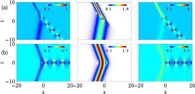
Figure 4. Amplitude profiles of (degenerate) two-soliton solutions formed by the nonlinear superposition of type-I and type-$I^{\prime} $ solitons. The case (a) shows a ‘fusion’ of type-I dark-bright solitons and a general breather when parameters are: α1 = α2 = 1, γ1 = γ2 = 1; The case (b) shows a ‘reflection’ of dark-bright solitons when parameters are: α1 = α2 = 0, γ1 = γ2 = 1. |
7. Composite solutions
Degenerate dark-bright solitons are tightly related to the composite solutions. The latter are the first-order solutions (18 ) when all three coefficients of the vector eigenfunction are nonzero, c1,l ≠ 0 (l = a, b, c). For simplicity, let c1,l = {1, 1, 1}.
For the sake of comparison with degenerate solutions in figure 4, we consider the composite solution with the same eigenvalue χa,1(α1, γ1). Figure 5 shows the amplitude profiles of the composite solutions with parameters α1, γ1, the same as in figure 4. Similar to the case of degenerate solutions, the composite solution is the interaction of three localized waves but the process is inverted in x and t. Instead of the ’fusion’ we observe ’fission’ of one soliton into two others in figure 5(a). The reflection in figure 5(b) is essentially the same as in figure 4(b) but occurs from the other end of Akhmediev breather.
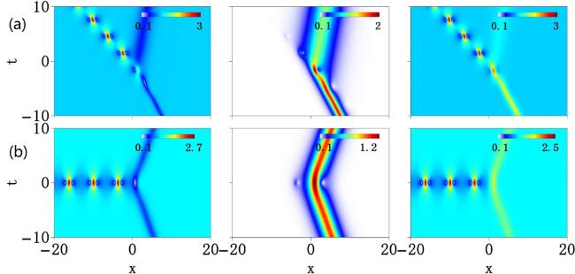
Figure 5. Amplitude profiles of the composite solution with the eigenvalue χa,1(α1, γ1) and c1,l ≠ 0 (l = a, b, c). (a) ‘Fission’ of type-$I^{\prime} $ dark-bright soliton with α1 = γ1 = 1. (b) ‘Reflection’ of dark-bright solitons with α1 = 0, γ1 = 1. |
8. Interaction of dark-bright solitons with equal velocity in the focusing case
The condition of equal velocities ${V}_{g,I}={V}_{g,I^{\prime} }$ leads to the condition γ1 = γ2 = 0. In this case, the two types of solitons have zero velocities. Then, the dark-bright soliton interaction depends on the relative separation of two solitons in x, defined by their positions (x1, x2). The bound states of solitons in this case are oscillating with complex amplitude profiles. These results are different from those in [39] where the dark-bright soliton interacts with the Peregrine rogue wave with a time-dependent velocity.
For simplicity, we take x1 = t1 = t2 = 0 and vary only x2 in order to control the relative separation. Figure 6 reveals the interaction patterns of type-I and type-$I^{\prime} $ dark-bright solitons (20 ). We fix two parameters α1, and α2. The corresponding solutions are: ${\psi }_{I}^{(j)}({\alpha }_{1})$ and ${\psi }_{I^{\prime} }^{(j)}({\alpha }_{2})$ .

Figure 6. Amplitude profiles of (nondegenerate) two-soliton solutions showing the interaction of type-I and type-$I^{\prime} $ dark-bright solitons with α1 ≠ α2. The relative separation of solitons in x are: (a) x2 = 10; (b) x2 = 3; (c) x2 = 0; (d) x2 = − 4.3; (e) x2 = − 20. Three panels from left to right show the individual components ∣$\Psi$(1)∣, ∣$\Psi$(2)∣, and the total amplitude $| \psi | =\sqrt{| {\psi }^{(1)}{| }^{2}+| {\psi }^{(1)}{| }^{2}}$ . Parameters are: α1 = 2, α2 = 3. |
When ∣x2∣ is large, the two dark-bright solitons are well separated. This case is shown in figures 6(a) and (e). The two solitons can be considered as independent. There is no beating in the soliton profiles. Reducing ∣x2∣ leads to the weak nonlinear interaction of two solitons resulting in their beating. Figure 6(b) shows the case when x2 = 3. In the $\Psi$(1) wave component, the dark-bright soliton on the left is clearly oscillating while the oscillations of the type-I dark soliton on the right are hardly visible. The $\Psi$(2) wave component as well as the total amplitude display a bright oscillating soliton on the left and type-I bright soliton on the right. A similar pattern can be observed in figure 6(c) except that the two solitons are closer to each other making the oscillations of the soliton on the left larger. Here, it can be seen that in each period of oscillations in the $\Psi$(1) component of the dark breather the pattern has the form of a four-petal structure.
The special case of the strongest soliton interaction is shown in figure 6(d). Here, x2 = −4.3. The amplitude profile pattern is symmetric in x. There is an oscillating bright soliton in the middle of the $\Psi$(1) component and two satellite dark solitons at each side of it. The $\Psi$(2) component and the total amplitude show a bright soliton with an oscillating central stripe. This pattern can be considered as the analog of the second-order soliton of Satsuma and Yajima [22] in the scalar case except that periodic beating is also influenced by the background field in the first component.
All three solutions $\Psi$(j)(α1, α2) shown in figures 6(b)–(d) have the same period of oscillations in t. It is roughly the same period as for the scalar Kuznetsov-Ma soliton (KMS) ${\psi }_{{\rm{KMS}}}^{(1)}$ given by the solution (A1 ) with α = α2. Namely,A1 ). One of the two peak amplitude curves shifted vertically relative to the other one. This is due to the background component of the solution shown in figure 6(d). Figure 7(d) shows the comparison of periods of the scalar KMS ${\psi }_{{\rm{KMS}}}^{(1)}({\alpha }_{2})$ and the two-soliton solution $\Psi$(j)(α1, α2) with different α1, as α2 increases. As can be seen from the figure, the periods of them show good agreement.
$\begin{eqnarray}{D}_{t}=\left|\displaystyle \frac{4\pi }{{\alpha }_{2}\sqrt{{\alpha }_{2}^{2}+4{a}^{2}}}\right|.\end{eqnarray}$
This is shown in figure 7(c) by comparing the curves of maximal amplitudes of $\Psi$(1)(α1, α2) shown in figure 6(d) and the scalar KMS ${\psi }_{{\rm{KMS}}}^{(1)}({\alpha }_{2})$ given by (
Figure 7. Amplitude profiles of the scalar Kuznetsov-Ma soliton ( |
9. Special case α1 = α2
The nonlinear superposition of type-I and type-$I^{\prime} $ solitons (20 ) with equal α $[{\psi }_{I}^{(j)}({\alpha }_{1})$ and ${\psi }_{I^{\prime} }^{(j)}({\alpha }_{1})]$ is special. Figure 8 shows the amplitude profiles of the solutions for this case. All solutions are oscillating in t. When x2 = 2 and x2 = 0, the solution shows an oscillating dark-bright breather as in figures 8(a) and (b), respectively. The soliton in $\Psi$(1)- and $\Psi$(2)-components have asymmetric profiles in x. The total amplitude $| \psi | =\sqrt{| {\psi }^{(1)}{| }^{2}+| {\psi }^{(1)}{| }^{2}}$ shows the features of the symmetric profile of breather. When x2 is negative and large, as in figure 8(c) both solitons appear within the window. One of them is the type-I dark-bright soliton ${\psi }_{I}^{(j)}({\alpha }_{1})$ , the other one is Kuznetsov-Ma soliton ${\psi }_{{\rm{KMS}}}^{(1)}({\alpha }_{1})$ given by the solution (A1 ).

Figure 8. Amplitude profiles of (degenerate) two-soliton solutions formed by nonlinear superposition of type-I and type-$I^{\prime} $ dark-bright solitons with α1 = α2 = 2. The relative separations in x are: (a) x2 = 2; (b) x2 = 0; (c) x2 = − 13. Three panels from left to right are the individual components ∣$\Psi$(1)∣, ∣$\Psi$(2)∣, and the total amplitude $| \psi | =\sqrt{| {\psi }^{(1)}{| }^{2}+| {\psi }^{(1)}{| }^{2}}$ . |
The oscillating solitons shown in figures 8(a)–(c) have the same period in t, which is given byA1 ) with α = α1. When α1 → 0, the period (34 ) of the oscillating soliton goes to infinity, and the solution reduces to a structure similar to the Peregrine rogue wave. Again, in this case, we have the interaction of the dark-bright soliton and a scalar rogue wave. It is similar to the fundamental composite solution reported in [37–40].
$\begin{eqnarray}{D}_{t}=\left|\displaystyle \frac{4\pi }{{\alpha }_{1}\sqrt{{\alpha }_{1}^{2}+4{a}^{2}}}\right|.\end{eqnarray}$
It is exactly the same period as for the scalar KMS ${\psi }_{{\rm{KMS}}}^{(1)}$ given by the solution (10. Numerical simulations
To confirm the validity of our exact solutions, we performed numerical simulations for the Manakov equations by using the split-step Fourier method. We first consider the initial condition for simulations given by the exact solutions at t = − 10, namely, $\Psi$(j)(x, t = − 10). Using such initial conditions, we were able to reproduce all exact solutions in numerical simulations. As an example, we show the results of numerical excitations of solitons in figure 9(a) where Akhmediev breathers are excited during the interaction between two solitons. As can be seen, the numerical results are in full agreement with the exact solutions shown in figure 3(d).

Figure 9. Numerical simulation of solitons shown in figure 3(d) starting from (a) the initial condition of exact solutions at t = −10, $\Psi$(j)(x, t = −10), and (b) the initial condition $\Psi$(j)(x, t = −10) perturbed by the white noise of a strength of 10−4. |
Figure 9(b) shows numerical excitations starting with the exact solutions $\Psi$(j)(x, t = − 10) perturbed by the white noise of a strength of 10−4. Clearly, the interaction between two solitons and the intermediate Akhmediev breathers are observed. Other periodic waves manifest because of the spontaneous modulation instability on the plane wave background. This result confirms the robustness of the exact solutions.
11. Conclusions
We studied fundamental dark-bright solitons and their interaction in both focusing and defocusing regimes of the Manakov equations. A unified form of fundamental soliton solutions of different types is given. Such solutions contain two types of solitons in the defocusing regime and four types of solitons in the focusing regime. Soliton interactions and their role in breather formation are investigated. We show that only special types of soliton interactions in the focusing regime can generate breathers. We demonstrate this phenomenon by considering such soliton interactions with equal and unequal velocities. Solutions that we derived suggest the initial conditions to generate breathers within two dark-bright solitons in vector nonlinear wave systems. This can be useful for experimental works in optics, hydrodynamics and cold atom physics.
We point out that Manakov equations also admit a class of beating solitons formed by linear superposition between fundamental dark-bright solitons via SU(2) rotations [57–60]. The dark-bright solitons obtained in the present paper will yield rich patterns of beating solitons [62]. This will be published elsewhere.
Acknowledgments
The work is supported by the NSFC (Grants Nos. 12175178 and 12247103), Shaanxi Fundamental Science Research Project for Mathematics and Physics (Grant No. 22JSY016), and Graduate innovation project of Northwest University (Grant No. CX2024137).
Appendix A. Fundamental breather solution
A fundamental breather on the plane wave background (6 ) exists only in the focusing regime of the Manakov equations. The solution follows from (18 ) when the coefficients of the vector eigenfunctions {c1,a, c1,b, c1,c} = {1, 1, 0}. The explicit form of the solution is given byA1 ) are given by:A1 ) of $\Psi$(1) consists of the following subfamilies. The set of general breathers when α ≠ 0, γ ≠ 0, a subset of Akhmediev breathers (AB) when α = 0, γ ≠ 0, a subset of Kuznetsov-Ma solitons when α ≠ 0, γ = 0. It includes the Peregrine rogue wave when α = γ = 0. The solutions have the following physical parameters. Akhmediev breathers are periodic in x with a period given by
$\begin{eqnarray}{\psi }_{}^{(1)}={\psi }_{0}^{(1)}\left(1+\displaystyle \frac{G}{H}\right),\,{\psi }^{(2)}=0,\end{eqnarray}$
where $\begin{eqnarray*}\begin{array}{rcl}G & = & {\mu }_{1}\cos {\rm{\Lambda }}+{\mu }_{1}\cosh {\rm{\Delta }}+{\rm{i}}{\mu }_{2}\sin {\rm{\Lambda }}+{\mu }_{2}\sinh {\rm{\Delta }},\\ H & = & {\mu }_{3}\cos {\rm{\Lambda }}+{\mu }_{4}\cosh {\rm{\Delta }}+{\rm{i}}{\mu }_{5}\sin {\rm{\Lambda }}+{\mu }_{6}\sinh {\rm{\Delta }},\end{array}\end{eqnarray*}$
and $\begin{eqnarray}\begin{array}{rcl}{\rm{\Lambda }} & = & -\gamma x+\displaystyle \frac{1}{2}\left[{\alpha }^{2}+2{\chi }_{{ai}}\alpha -\gamma (2{\chi }_{{ar}}+\gamma )\right]t,\\ {\rm{\Delta }} & = & \alpha x+\left[{\chi }_{{ai}}\gamma +\alpha ({\chi }_{{ar}}+\gamma )\right]t.\end{array}\end{eqnarray}$
Parameters μi in equation ( $\begin{eqnarray*}\begin{array}{rcl}{\mu }_{1} & = & \displaystyle \frac{1}{{\chi }_{a}}+\displaystyle \frac{1}{{\chi }_{b}},\,{\mu }_{2}=\displaystyle \frac{1}{{\chi }_{a}}-\displaystyle \frac{1}{{\chi }_{b}},\\ {\mu }_{3} & = & 2+\displaystyle \frac{{a}^{2}}{{\chi }_{a}^{\ast }{\chi }_{b}}+\displaystyle \frac{{a}^{2}}{{\chi }_{a}{\chi }_{b}^{\ast }},\,{\mu }_{4}=2+\displaystyle \frac{{a}^{2}}{| {\chi }_{a}{| }^{2}}+\displaystyle \frac{{a}^{2}}{| {\chi }_{b}{| }^{2}},\\ {\mu }_{5} & = & \displaystyle \frac{{a}^{2}}{{\chi }_{a}{\chi }_{b}^{\ast }}-\displaystyle \frac{{a}^{2}}{{\chi }_{a}^{\ast }{\chi }_{b}},\,{\mu }_{6}=\displaystyle \frac{{a}^{2}}{{\chi }_{a}{\chi }_{a}^{\ast }}-\displaystyle \frac{{a}^{2}}{{\chi }_{b}{\chi }_{b}^{\ast }}.\end{array}\end{eqnarray*}$
The family of solutions ( $\begin{eqnarray}{D}_{x}=\left|\displaystyle \frac{2\pi }{\gamma }\right|,\end{eqnarray}$
where γ ∈ ( − 2a, 2a) is the initial modulation frequency. The growth rate of the AB also depends on γ: $\begin{eqnarray}\left|\gamma \sqrt{4{a}^{2}-{\gamma }^{2}}\right|.\end{eqnarray}$
Kuznetsov-Ma soliton is periodic in t. The corresponding period is given by $\begin{eqnarray}{D}_{t}=\left|\displaystyle \frac{4\pi }{\alpha \sqrt{{\alpha }^{2}+4{a}^{2}}}\right|.\end{eqnarray}$
Appendix B. Vector two-soliton solutions
The exact two dark-bright soliton solutions of the Manakov system (1 ) can be obtained at the second step of the Darboux transformation starting with the fundamental soliton solution (20 ). The corresponding eigenfunctions $\Psi$2=${({R}_{2},{S}_{2},{W}_{2})}^{{\mathsf{T}}}$ (n = 2) of the Lax pair (3 ) are
$\begin{eqnarray}\begin{array}{rcl}{R}_{2} & = & {\varphi }_{2,a}+{\varphi }_{2,b},\\ {S}_{2} & = & {\psi }_{0}^{(1)}\left(\displaystyle \frac{{\varphi }_{2,a}}{{\chi }_{2,a}}+\displaystyle \frac{{\varphi }_{2,b}}{{\chi }_{2,b}}\right),\\ {W}_{2} & = & {\varphi }_{2,c}.\end{array}\end{eqnarray}$
The two-soliton solution can be written as $\begin{eqnarray}{\psi }_{2}^{(1)}={\psi }_{1}^{(1)}+({\lambda }_{2}^{\ast }-{\lambda }_{2}){\left(P\right)}_{12},\end{eqnarray}$
$\begin{eqnarray}{\psi }_{2}^{(2)}={\psi }_{1}^{(2)}+({\lambda }_{2}^{\ast }-{\lambda }_{2}){\left(P\right)}_{13}.\end{eqnarray}$
Here, ${\psi }_{1}^{(j)}$ denote the fundamental solution, ${\left(P\right)}_{1i}$ represents the matrix element (P) in the first row and i column, and $\begin{eqnarray}T=I-\displaystyle \frac{{\lambda }_{1}-{\lambda }_{1}^{\ast }}{{\lambda }_{2}-{\lambda }_{1}^{\ast }}\displaystyle \frac{{{\rm{\Psi }}}_{1}{{\rm{\Psi }}}_{1}^{\dagger }}{{{\rm{\Psi }}}_{1}^{\dagger }{{\rm{\Psi }}}_{1}},\end{eqnarray}$
$\begin{eqnarray}P=\displaystyle \frac{{{\rm{\Psi }}}_{2}{{\rm{\Psi }}}_{2}^{\dagger }}{{{\rm{\Psi }}}_{2}^{\dagger }{{\rm{\Psi }}}_{2}},\,\,\,{{\rm{\Psi }}}_{2}=T{{\rm{\Psi }}}_{2},\end{eqnarray}$
where † denotes the matrix transpose and complex conjugate. For the two solitons in the defocusing regime shown in figure 1, we take λ1 = λ(χa,1) and λ2 = λ(χa,2). For the two solitons in the focusing regime (e.g. shown in figure 3), we take λ1 = λ2 = λ(χa,1).