


1. Introduction
From the earliest algorithms for factoring large numbers [1] and unstructured database searching [2], to algorithms for linear systems of equations [3] and quantum machine learning [4], quantum computing has demonstrated its tremendous computational advantages. However, the realization of some quantum algorithms that require large-depth quantum circuits consisting of high-precision quantum gates is still difficult in the current era of noisy intermediate-scale quantum (NISQ) devices [5]. Existing quantum devices contain about 100 physical qubits, which is not perfect since the qubits and quantum operations supported by NISQ devices are not error corrected [6]. Even without error correction, noise in shallow circuit implementations can be suppressed by error mitigation [7, 8], suggesting that it is feasible to utilize NISQ hardware for quantum computing. Most of the current NISQ algorithms delegate the classically difficult part of the computation to a quantum computer, while the other part of the computation is performed on a sufficiently powerful classical device. These types of quantum algorithms are known as variational quantum algorithms (VQAs) [6]. The earliest VQAs can be traced back to the variational quantum eigensolver [9] and quantum approximate optimization algorithm [10]. Later, inspired by the existing algorithms, VQAs in various fields, such as machine learning and quantum information, were proposed.
The Poisson equation has important applications in many areas of science and engineering, such as computational fluid dynamics [11] and the theory of Markov chains [12, 13], and is also important for density functional theory and electronic structure calculations [14]. It is therefore very interesting to explore how the Poisson equation can be solved on NISQ devices. In general, the Poisson equation is discretized using methods such as the finite-difference method [15] to obtain a linear system whose solution approximates the Poisson equation. VQAs for solving linear systems on near-term quantum devices have been proposed [16–20]. Most of these VQAs assume that the coefficient matrix of the linear system can consist of a polynomial number (with respect to the number of qubits) of tensor products of the local operator, such as I, σX, σY, σZ. For general linear systems, finding a strategy that satisfies the above requirements is a nontrivial problem. Based on the structure of the coefficient matrix of the discretized Poisson equation, work has been done to design relevant VQAs in a targeted manner. The authors in [21] find an explicit tensor product decomposition of a coefficient matrix under a set of simple operators {I, σ+ = ∣0⟩⟨1∣, σ− = ∣1⟩⟨0∣}, with only $(2\mathrm{log}2n+1)$ items, where n is the dimension of the coefficient matrix A. Inspired by [21], the authors in [22] develop a method for decomposing matrices based on the sigma basis. Sato et al [23] propose a VQA based on minimal potentials to solve the Poisson equation, which decomposes the corresponding observations into linear combinations of the tensor product of Pauli operators and simple observables. In [24], the authors rewrite the cost function as a quantity related to σX ⨂ A and decompose σX ⨂ A into a sum of Hermitian, one-sparse and self-inverse operators. Then, for the one-dimensional Poisson equation with different boundary conditions and for the d-dimensional Poisson equation with Dirichlet boundary conditions, σX ⨂ A is decomposed into a sum of, at most, seven terms and 4d + 1 terms, respectively, and σX ⨂ A2 is decomposed into a sum of at most 15 terms and (4d + 1)2−(4d + 1) terms, respectively. And the number of terms in the sparse matrix factorization is independent of the coefficient matrix dimension n.
In this paper, we present a different decomposition strategy to reduce the number of the decomposition terms for solving the Poisson equation on NISQ devices. We transform the matrix A into the banded Toeplitz matrix and give a VQA for the banded Toeplitz system. Then, for the one-dimensional Poisson equation with different boundary conditions, we decompose the corresponding Hamiltonian into, at most, five and six terms. Similarly, the corresponding Hamiltonian of the d-dimensional Poisson equation with Dirichlet boundary conditions can be decomposed into, at most, 4d + 1 and 12d2. Naturally, the decomposition method and the quantum circuit design remain applicable for a linear system with Hermitian and sparse coefficient matrices satisfying ai,i+c = ac for c = 0, 1, ⋯ ,n − 1 and i = 0, ⋯ ,n − 1 − c, where ai,i+c denotes the element of matrix A.
The remainder of the paper is organized as follows. In section 2 , we briefly review the definition of the Poisson equation, the discretized Poisson equation and the definition of the corresponding cost function. In section 3 , we expound how to approximate the ground state of the Hamiltonian using a VQA based on the decomposition of A and A2, and numerically illustrate the performance of our algorithm for the one-dimensional Poisson equation with Dirichlet boundary conditions. We generalize the algorithm of the Poisson equation to the banded Toeplitz matrix in section 4 . Finally, we present our conclusion and discussion in section 5 .
2. The VQA for the Poisson equation
The one-dimensional Poisson equation with different boundary conditions [21, 24] can be written as
$\begin{eqnarray*}-\bigtriangleup \mu (x)=f(x),x\in (0,1),\end{eqnarray*}$
with the unified boundary conditions ${\alpha }_{1}\mu ^{\prime} (0)-{\alpha }_{2}\mu (0)=0$ and ${\beta }_{1}\mu ^{\prime} (0)-{\beta }_{2}\mu (0)=0$ , where △ is the Laplace operator; α1, α2, β1 and β2 are all positive constants; and f: D → R is a sufficiently smooth function. The d-dimensional Poisson equation with Dirichlet boundary conditions is of the form −△μ(x) = f(x), x ∈ (0, 1)d with the boundary conditions μ(x) = 0, x ∈ {0, 1}d.Via the finite-difference method, the discretized one-dimensional Poisson equation with the unified boundary conditions is
$\begin{eqnarray*}\tilde{A}x=b,\end{eqnarray*}$
where $\begin{eqnarray*}\tilde{A}=\left[\begin{array}{cccc}2-c & -1 & \cdots & 0\\ -1 & \ddots & \ddots & \vdots \\ \vdots & \ddots & \ddots & -1\\ 0 & \cdots & -1 & 2-d\end{array}\right]\in {R}^{n\,\times \,n},\end{eqnarray*}$
and $c=\tfrac{{\alpha }_{1}}{{\alpha }_{1}+{\alpha }_{2}h}$ , $d=\tfrac{{\beta }_{1}}{{\beta }_{1}+{\beta }_{2}h}$ , $h=\tfrac{1}{n+1}$ , n comes from evenly dividing (0, 1) into n + 1 parts during the discretization, and b ∈ Rn is the vector obtained by sampling f(x) on the interior grid points. For simplicity, we assume that n = 2N, where N is a positive integer. Similarly, we can also obtain the coefficient matrix generated by the discretization of the d-dimensional Poisson equation with Dirichlet boundary conditions, $\begin{eqnarray*}\begin{array}{l}{A}^{\left(d\right)}=A^{\prime} \otimes I\otimes ...\otimes I+I\otimes A^{\prime} \otimes I\otimes \\ ...\otimes I\,+\,\cdots +\,I\otimes \cdots \otimes I\otimes A^{\prime} ,\end{array}\end{eqnarray*}$
where $\begin{eqnarray*}A^{\prime} =\left[\begin{array}{cccc}2 & -1 & \cdots & 0\\ -1 & \ddots & \ddots & \vdots \\ \vdots & \ddots & \ddots & -1\\ 0 & \cdots & -1 & 2\end{array}\right]\in {R}^{n\,\times \,n},\end{eqnarray*}$
I ∈ Rn×n and ${A}^{\left(d\right)}\in {R}^{{n}^{d}\,\times \,{n}^{d}}$ .As with most VQAs for solving a linear system Ax = b, we transform it to find the ground state of a Hamiltonian H,
$\begin{eqnarray*}H={A}^{\dagger }(I-| b\rangle \langle b| )A,\end{eqnarray*}$
where $\left|b\right\rangle \propto b$ , A is the coefficient matrix of the linear system. And we assume that there is an efficient unitary operator Ub that can prepare a quantum state $\left|b\right\rangle $ . It is easy to verify that the solution $\left|x\right\rangle $ of a linear system is the unique eigenstate corresponding to the minimum eigenvalue 0 of the Hamiltonian H.To obtain $\left|x\right\rangle $ , we define the cost function E(θ) = ⟨$\Psi$(θ)∣H∣$\Psi$(θ)⟩, where ∣$\Psi$(θ)⟩ = U(θ)∣0⟩, with a unitary gate $U(\theta )\,={\prod }_{i=1}^{d}{\otimes }_{t=1}^{N}U({\theta }_{t}^{i}){W}_{i}$ , where $U({\theta }_{t}^{i})$ is a product of combinations of single-qubit rotational gates, $\theta =[{\theta }_{1}^{0},\ldots ,{\theta }_{N}^{0},\ldots ,{\theta }_{1}^{d},\ldots ,{\theta }_{N}^{d}]$ , d is the depth of the quantum circuit, ${\theta }_{t}^{i}\in [0,2\pi ]$ and Wi is composed of a nearest-neighbor controlled-NOT (CNOT) gate or controlled-σZ (CZ) gate The cost function E(θ) represents the expectation value of H under the state ∣$\Psi$(θ)⟩. Then, we aim to optimize the parameters θ to minimize E(θ), that is,
$\begin{eqnarray*}\begin{array}{rcl}\mathop{\min }\limits_{\theta }E(\theta ) & = & \mathop{\min }\limits_{\theta }\langle \psi (\theta )| H| \psi (\theta )\rangle \\ & = & \mathop{\min }\limits_{\theta }[\langle \psi (\theta )| {A}^{2}| \psi (\theta )\rangle -{\left|\langle b| A| \psi (\theta )\rangle \right|}^{2}].\end{array}\end{eqnarray*}$
To design a VQA for the Poisson equation, we give the decomposition based on the characterization of the matrices A and A2.
3. An explicit decomposition of A and A2
3.1. One-dimensional Poisson equation
Before decomposing the matrices A and A2, we introduce a special class of matrices, i.e. Toeplitz matrices [25, 26]. The Toeplitz matrix Tn is a matrix of size n × n, whose elements along each diagonal are constant. More clearly,
$\begin{eqnarray*}{T}_{n}=\left[\begin{array}{ccccc}{t}_{0} & {t}_{-1} & {t}_{-2} & \cdots & {t}_{-(n-1)}\\ {t}_{1} & {t}_{0} & {t}_{-1} & \cdots & {t}_{-(n-2)}\\ {t}_{2} & {t}_{1} & {t}_{0} & \ddots & \vdots \\ \vdots & \ddots & \ddots & \ddots & {t}_{-1}\\ {t}_{(n-1)} & \cdots & {t}_{2} & {t}_{1} & {t}_{0}\end{array}\right],\end{eqnarray*}$
where ti,k = ti−k and Tn is decided with 2n − 1 elements, i.e. $\{{t}_{j}\}{}_{j=-(n-1)}^{n-1}$ . Specifically, when tj = 0, j = ± (K + 1),…, ± (n − 1), Tn is a banded Toeplitz matrix TnK, namely, a 2K + 1-sparse diagonal matrix.The circulant matrix is a special form of the Toeplitz matrix. Its form is
$\begin{eqnarray*}{C}_{n}=\left[\begin{array}{ccccc}{c}_{0} & {c}_{n-1} & {c}_{n-2} & \cdots & {c}_{1}\\ {c}_{1} & {c}_{0} & {c}_{n-1} & \cdots & {c}_{2}\\ {c}_{2} & {c}_{1} & {c}_{0} & \ddots & \vdots \\ \vdots & \ddots & \ddots & \ddots & {c}_{n-1}\\ {c}_{n-1} & \cdots & {c}_{2} & {c}_{1} & {c}_{0}\end{array}\right].\end{eqnarray*}$
When cK+1, cK+2,…,cn−K−1 = 0, Cn is a 2K + 1-sparse matrix CnK. In this paper, it is necessary to rely on a special kind of circulant matrix, i.e. the unit circulant matrix:
$\begin{eqnarray*}L=\left[\begin{array}{ccccc}0 & 0 & \cdots & 0 & 1\\ 1 & 0 & & & 0\\ \vdots & \ddots & \ddots & & \vdots \\ \vdots & & 1 & 0 & 0\\ 0 & \cdots & \cdots & 1 & 0\end{array}\right],\end{eqnarray*}$
$\begin{eqnarray*}R=\left[\begin{array}{ccccc}0 & 1 & \cdots & 0 & 0\\ 0 & 0 & 1 & & 0\\ \vdots & & \ddots & \ddots & \vdots \\ 0 & & & 0 & 1\\ 1 & 0 & \cdots & 0 & 0\end{array}\right].\end{eqnarray*}$
Note that L† = R = L−1 and Ln−l = L−l, and
$\begin{eqnarray*}\begin{array}{rcl}{C}_{n}^{K} & = & \displaystyle \sum _{l=0}^{K}{c}_{l}{L}^{l}+\displaystyle \sum _{\imath =1}^{K}{c}_{n-\imath }{R}^{\imath }\\ & = & \displaystyle \sum _{\displaystyle \genfrac{}{}{0em}{}{l=0}{l\ne K+1,\ldots ,n-K+1}}^{N-1}\,{c}_{l}{L}^{l}=\displaystyle \sum _{l=-K}^{K}{c}_{l}{L}^{l},\end{array}\end{eqnarray*}$
where c−l = cn−l. Any circulant matrix Cn can be decomposed as $\begin{eqnarray*}{C}_{n}={F}_{n}^{-1}\mathrm{diag}({F}_{n}c){F}_{n},\end{eqnarray*}$
where the matrix Fn is a Fourier transform of order n and the vector c = [c0, c1,…,cn−1] is the first column of the circulant matrix Cn. In particular, for the unit circulant matrix L, one has $L={F}_{n}^{-1}{{DF}}_{n}$ , where $\begin{eqnarray*}D=\mathrm{diag}\{{\omega }_{n}^{0},{\omega }_{n}^{1},\cdots ,{\omega }_{n}^{n-1}\},\end{eqnarray*}$
${\omega }_{n}^{i}$ is the nth unit root, and can also be written as $\begin{eqnarray*}D=\left(\begin{array}{cc}1 & 0\\ 0 & {\omega }_{n}^{n/2}\end{array}\right)\otimes ...\otimes \left(\begin{array}{cc}1 & 0\\ 0 & {\omega }_{n}^{2}\end{array}\right)\otimes \left(\begin{array}{cc}1 & 0\\ 0 & {\omega }_{n}^{0}\end{array}\right)={\otimes }_{j=0}^{N-1}P({\theta }_{j}),\end{eqnarray*}$
where $\begin{eqnarray*}P(\theta )=\left[\begin{array}{cc}1 & 0\\ 0 & {{\rm{e}}}^{{\rm{i}}\theta }\end{array}\right],\end{eqnarray*}$
${\theta }_{j}=\tfrac{2\pi }{n}{2}^{j}$ . Thus, by computing the expectation of a Toeplitz matrix, Tn can be obtained by embedding it in a 2n × 2n circulant matrix C2n, i.e. $\begin{eqnarray*}{C}_{2n}=\left[\begin{array}{cc}{T}_{n} & {B}_{n}\\ {B}_{n} & {T}_{n}\end{array}\right],\end{eqnarray*}$
where $\begin{eqnarray*}{B}_{n}=\left[\begin{array}{ccccc}0 & {t}_{n-1} & \cdots & {t}_{2} & {t}_{1}\\ {t}_{-(n-1)} & 0 & {t}_{n-1} & \cdots & {t}_{2}\\ \vdots & {t}_{n-1} & 0 & \ddots & \vdots \\ {t}_{-2} & & \ddots & \ddots & {t}_{n-1}\\ {t}_{-1} & {t}_{-2} & \cdots & {t}_{-(n-1)} & 0\end{array}\right].\end{eqnarray*}$
Then, the expectation value of the circulant matrix CnK can be expressed as
$\begin{eqnarray*}\begin{array}{rcl}\langle \psi (\theta )| {C}_{n}^{K}| \psi (\theta )\rangle & = & \displaystyle \sum _{l=-K}^{K}{c}_{l}\langle \psi (\theta )| {L}^{l}| \psi (\theta )\rangle \\ & = & \displaystyle \sum _{l=-K}^{K}{c}_{l}\langle \psi (\theta )| {F}_{n}^{-1}{D}^{l}{F}_{n}| \psi (\theta )\rangle ,\end{array}\end{eqnarray*}$
where $\begin{eqnarray*}{D}^{l}=\mathrm{diag}\{{\left({\omega }_{n}^{0}\right)}^{l},{\left({\omega }_{n}^{1}\right)}^{l},\cdots ,{\left({\omega }_{n}^{n-1}\right)}^{l}\}.\end{eqnarray*}$
We will show the decompositions of matrices A and A2 according to the special structures. The main idea is to transform them into banded Toeplitz matrices for solving, and this process produces sparse matrices with only a small number of non-zero elements, for which we will make use of the extended Bell measurements method [27].
In particular, when the one-dimensional Poisson equation has Dirichlet boundary conditions, the matrix of the corresponding linear system is $A^{\prime} $ , which is a general tridiagonal Toeplitz matrix Tn1.
Thus, ${\left|\langle b| A^{\prime} | \psi (\theta )\rangle \right|}^{2}$ can be obtained by computing ${\left|\langle 0,b| {C}_{A^{\prime} }| 0,\psi (\theta )\rangle \right|}^{2}$ :
$\begin{eqnarray}\begin{array}{l}{\left|\langle b| A^{\prime} | \psi (\theta )\rangle \right|}^{2}\\ \ \ =\,{\left|\langle b| {T}_{n}^{1}| \psi (\theta )\rangle \right|}^{2}={\left|\langle 0,b| {C}_{{T}_{n}^{1}}| 0,\psi (\theta )\rangle \right|}^{2}\\ =| -\langle 0,b| {F}_{n}^{-1}{{DF}}_{n}| 0,\psi (\theta )\rangle \\ -\langle 0,b| {F}_{n}^{-1}{D}^{2n-1}{F}_{n}| 0,\psi (\theta )\rangle +2\langle 0,b| 0,\psi (\theta )\rangle {| }^{2},\end{array}\end{eqnarray}$
where $\begin{eqnarray*}{C}_{A^{\prime} }=\left[\begin{array}{cc}A^{\prime} & B\{A^{\prime} \}{}_{n}\\ B\{A^{\prime} \}{}_{n} & A^{\prime} \end{array}\right],\end{eqnarray*}$
$\begin{eqnarray*}B\{A^{\prime} \}{}_{n}=\left[\begin{array}{ccccc}0 & 0 & \cdots & 0 & -1\\ 0 & 0 & 0 & \ddots & 0\\ \vdots & & \ddots & & \vdots \\ 0 & & & \ddots & 0\\ -1 & 0 & \cdots & 0 & 0\end{array}\right].\end{eqnarray*}$
Similarly, $A{{\prime} }^{2}$ can be expressed as
$\begin{eqnarray*}\begin{array}{rcl}A{{\prime} }^{2} & = & \left[\begin{array}{cccccc}5 & -4 & 1 & & & 0\\ -4 & 6 & -4 & 1 & & \\ 1 & \ddots & \ddots & \ddots & \ddots & \\ & \ddots & \ddots & \ddots & \ddots & 1\\ & & 1 & -4 & 6 & -4\\ & & & 1 & -4 & 5\end{array}\right]\\ & = & \left[\begin{array}{cccccc}6 & -4 & 1 & & & 0\\ -4 & 6 & -4 & 1 & & \\ 1 & \ddots & \ddots & \ddots & \ddots & \\ & \ddots & \ddots & \ddots & \ddots & 1\\ & & 1 & -4 & 6 & -4\\ & & & 1 & -4 & 6\end{array}\right]-\left[\begin{array}{cccccc}1 & & & & & \\ & 0 & & & & \\ & & \ddots & & & \\ & & & \ddots & & \\ & & & & 0 & \\ & & & & & 1\end{array}\right]\\ & = & {T}_{n}^{2}-{M}_{1}.\end{array}\end{eqnarray*}$
And $\langle \psi (\theta )| A{{\prime} }^{2}| \psi (\theta )\rangle $ can be obtained by calculating
$\begin{eqnarray*}\begin{array}{l}\langle \psi (\theta )| {T}_{n}^{2}-{M}_{1}| \psi (\theta )\rangle \\ \quad =\,\langle \psi (\theta )| {T}_{n}^{2}| \psi (\theta )\rangle -\langle \psi (\theta )| {M}_{1}| \psi (\theta )\rangle ,\end{array}\end{eqnarray*}$
$\begin{eqnarray}\begin{array}{rcl}\langle \psi (\theta )| {T}_{n}^{2}| \psi (\theta )\rangle & = & \langle 0,\psi (\theta )| {C}_{{T}_{n}^{2}}| 0,\psi (\theta )\rangle \\ & = & -4\langle 0,\psi (\theta )| {F}_{n}^{-1}{{DF}}_{n}| 0,\psi (\theta )\rangle \\ & & +\langle 0,\psi (\theta )| {F}_{n}^{-1}{D}^{2}{F}_{n}| 0,\psi (\theta )\rangle \\ & & -4\langle 0,\psi (\theta )| {F}_{n}^{-1}{D}^{2n-1}{F}_{n}| 0,\psi (\theta )\rangle \\ & & +\langle 0,\psi (\theta )| {F}_{n}^{-1}{D}^{2n-2}{F}_{n}| 0,\psi (\theta )\rangle +6\\ & = & -4\langle 0,\psi (\theta )| {F}_{n}^{-1}{{DF}}_{n}| 0,\psi (\theta )\rangle \\ & & +\langle 0,\psi (\theta )| {F}_{n}^{-1}{D}^{2}{F}_{n}| 0,\psi (\theta )\rangle \\ & & -4\overline{\langle 0,\psi (\theta )| {F}_{n}^{-1}{{DF}}_{n}| 0,\psi (\theta )\rangle }\\ & & +\overline{\langle 0,\psi (\theta )| {F}_{n}^{-1}{D}^{2}{F}_{n}| 0,\psi (\theta )\rangle }+6,\end{array}\end{eqnarray}$
where $\begin{eqnarray*}{C}_{{T}_{n}^{2}}=\left[\begin{array}{cc}{T}_{n}^{2} & B\{{T}_{n}^{2}\}{}_{n}\\ B\{{T}_{n}^{2}\}{}_{n} & {T}_{n}^{2}\end{array}\right],\end{eqnarray*}$
$\begin{eqnarray*}B\{{T}_{n}^{2}\}{}_{n}=\left[\begin{array}{cccccc}0 & 0 & & & 1 & -4\\ 0 & 0 & & & 0 & 1\\ & \ddots & \ddots & \ddots & \ddots & \\ & \ddots & \ddots & \ddots & \ddots & \\ 1 & 0 & & & 0 & 0\\ -4 & 1 & & & 0 & 0\end{array}\right].\end{eqnarray*}$
For the sparse matrix M1, due to the specificity (symmetry) of the positions of its non-zero elements, we can construct the associated quantum circuit. We take n = 8 (N = 3), for example, to illustrate the quantum circuit. The matrix M1 can be rearranged as
$\begin{eqnarray*}\begin{array}{rcl}{M}_{1} & = & | 000\rangle \langle 000| +| 111\rangle \langle 111| \\ & = & \displaystyle \frac{1}{2}(| 000\rangle +| 111\rangle )(\langle 000| +\langle 111| )\\ & & +\displaystyle \frac{1}{2}(| 000\rangle -| 111\rangle )(\langle 000| -\langle 111| )\\ & = & ({\mathrm{CNOT}}_{2}^{0}{\mathrm{CNOT}}_{1}^{0}{H}^{0}| 000\rangle )\\ & & \times \,{\left({\mathrm{CNOT}}_{2}^{0}{\mathrm{CNOT}}_{1}^{0}{H}^{0}| 000\rangle \right)}^{\dagger }\\ & & +({\mathrm{CNOT}}_{2}^{0}{\mathrm{CNOT}}_{1}^{0}{H}^{0}{X}^{0}| 000\rangle )\\ & & \times \,{\left({\mathrm{CNOT}}_{2}^{0}{\mathrm{CNOT}}_{1}^{0}{H}^{0}{X}^{0}| 000\rangle \right)}^{\dagger },\end{array}\end{eqnarray*}$
where Gji represents the quantum gate G applied at the jth qubit controlled by the ith qubit, such as the fact that ${\mathrm{CNOT}}_{j}^{i}$ is the CNOT gate whose control and target qubits are ith and jth qubits, respectively.Thus, for ⟨$\Psi$(θ)∣M1∣$\Psi$(θ)⟩, we have
$\begin{eqnarray*}\begin{array}{l}\langle \psi (\theta )| {M}_{1}| \psi (\theta )\rangle \\ \ \ \ \ \ =\,\langle \psi (\theta )| ({\mathrm{CNOT}}_{2}^{0}{\mathrm{CNOT}}_{1}^{0}{H}^{0}| 000\rangle )\\ \ \ \ \ \ \times \,{\left({\mathrm{CNOT}}_{2}^{0}{\mathrm{CNOT}}_{1}^{0}{H}^{0}| 000\rangle \right)}^{\dagger }\\ +\,({\mathrm{CNOT}}_{2}^{0}{\mathrm{CNOT}}_{1}^{0}{H}^{0}{X}^{0}| 000\rangle )\\ \ \ \ \ \ \times \,{\left({\mathrm{CNOT}}_{2}^{0}{\mathrm{CNOT}}_{1}^{0}{H}^{0}{X}^{0}| 000\rangle \right)}^{\dagger }| \psi (\theta )\rangle \\ =\,| \langle \psi (\theta )| {\mathrm{CNOT}}_{2}^{0}{\mathrm{CNOT}}_{1}^{0}{H}^{0}| 000\rangle {| }^{2}\\ \ \ \ \ \ +\,\,| \langle \psi (\theta )| {\mathrm{CNOT}}_{2}^{0}{\mathrm{CNOT}}_{1}^{0}{H}^{0}{X}^{0}| 000\rangle {| }^{2}.\\ \end{array}\end{eqnarray*}$
The quantum circuit of the one-dimensional Poisson equation with Dirichlet boundary conditions is shown in figure 1.

Figure 1. The quantum circuits for estimating the values of the cost function E(θ). (a) The Hadamard test circuit to estimate the items $\langle 0,\psi (\theta )| {F}_{n}^{-1}{D}^{l}{F}_{n}| 0,\psi (\theta )\rangle $ . The QFT gate in the quantum circuit represents the Quantum Fourier Transform. (b) The Hadamard test circuit to estimate the items $\langle 0,b| {F}_{n}^{-1}{D}^{l}{F}_{n}| 0,\psi (\theta )\rangle $ . (c) The detailed structure of the unitary matrix Ll. (d) The quantum circuit for estimating ⟨$\Psi$(θ)∣M1∣$\Psi$(θ)⟩. ⟨$\Psi$(θ)∣M1∣$\Psi$(θ)⟩ can be evaluated by the probabilities of obtaining bit-strings 000 when measuring ${H}^{0}{\mathrm{CNOT}}_{1}^{0}{\mathrm{CNOT}}_{2}^{0}| \psi (\theta )\rangle $ and ${X}^{0}{H}^{0}{\mathrm{CNOT}}_{1}^{0}{\mathrm{CNOT}}_{2}^{0}| \psi (\theta )\rangle $ in the computational basis. |
When the Poisson equation has the unified boundary conditions, the matrix of the corresponding linear system is $\tilde{A}$ . Decomposing $\tilde{A}$ , we have
$\begin{eqnarray*}\begin{array}{rcl}\tilde{A} & = & \left[\begin{array}{ccccc}2 & -1 & \cdots & 0 & 0\\ -1 & 2 & -1 & \ddots & 0\\ \vdots & & \ddots & & \vdots \\ 0 & & & \ddots & -1\\ 0 & 0 & \cdots & -1 & 2\end{array}\right]-c\left[\begin{array}{cccc}1 & 0 & \cdots & 0\\ 0 & \ddots & \ddots & \vdots \\ \vdots & \ddots & \ddots & 0\\ 0 & \cdots & 0 & 0\end{array}\right]-d\left[\begin{array}{cccc}0 & 0 & \cdots & 0\\ 0 & \ddots & \ddots & \vdots \\ \vdots & \ddots & \ddots & 0\\ 0 & \cdots & 0 & 1\end{array}\right]\\ & = & A^{\prime} -{{cM}}_{2}-{{dM}}_{3}\\ & = & {T}_{n}^{1}-{{cM}}_{2}-{{dM}}_{3}.\end{array}\end{eqnarray*}$
Similarly, we can obtain the decomposition of ${\tilde{A}}^{2}$ as
$\begin{eqnarray*}{\tilde{A}}^{2}=\left[\begin{array}{cccccc}6-4c-1+{c}^{2} & -4+c & 1 & & & 0\\ -4+c & 6 & -4 & 1 & & \\ 1 & \ddots & \ddots & \ddots & \ddots & \\ & \ddots & \ddots & \ddots & \ddots & 1\\ & & 1 & -4 & 6 & -4+d\\ & & & 1 & -4+d & 6-4d-1+{d}^{2}\end{array}\right]\end{eqnarray*}$
$\begin{eqnarray*}\begin{array}{l}=\left[\begin{array}{cccccc}6 & -4 & 1 & & & 0\\ -4 & 6 & -4 & 1 & & \\ 1 & \ddots & \ddots & \ddots & \ddots & \\ & \ddots & \ddots & \ddots & \ddots & 1\\ & & 1 & -4 & 6 & -4\\ & & & 1 & -4 & 6\end{array}\right]\\ -\left[\begin{array}{cccccc}4c+1-{c}^{2} & & & & & \\ & 0 & & & & \\ & & \ddots & & & \\ & & & \ddots & & \\ & & & & 0 & \\ & & & & & 4d+1-{d}^{2}\end{array}\right]\\ +\,c\left[\begin{array}{cccccc}0 & 1 & 0 & & & 0\\ 1 & 0 & 0 & & & 0\\ 0 & \ddots & \ddots & \ddots & \ddots & \\ & \ddots & \ddots & \ddots & \ddots & 0\\ & & & & 0 & 0\\ & & & 0 & 0 & 0\end{array}\right]+d\left[\begin{array}{cccccc}0 & 0 & 0 & & & 0\\ 0 & 0 & 0 & & & 0\\ 0 & \ddots & \ddots & \ddots & \ddots & \\ & \ddots & \ddots & \ddots & \ddots & 0\\ & & & & 0 & 1\\ & & & 0 & 1 & 0\end{array}\right]\\ =\,{T}_{n}^{2}-(4c+1-{c}^{2}){M}_{2}-(4d+1-{d}^{2}){M}_{3}+{{cM}}_{4}+{{dM}}_{5}.\end{array}\end{eqnarray*}$
$\begin{eqnarray*}\end{eqnarray*}$
To summarize, for the one-dimensional Poisson equation with different boundary conditions, the number of decomposition terms of $\langle b| \tilde{A}| \psi (\theta )\rangle $ is five, and the number of decomposition terms of $\langle \psi (\theta )| {\tilde{A}}^{2}| \psi (\theta )\rangle $ is six. We provide the algorithm flowchart in figure 2 for a more detailed presentation. The implementation of Tn1 and Tn2 is consistent with the previously mentioned approach, i.e. equations (1 ) and (2 ). Obviously, it is easy to obtain ⟨b∣Mj∣$\Psi$(θ)⟩, j = {1, 2}. As described earlier, ⟨$\Psi$(θ)∣Mj∣$\Psi$(θ)⟩, j ∈ {4, 5} can be obtained from the extended Bell measurements method. We take n = 8 (N = 3), for example, to illustrate the specific quantum circuits too. The matrices can be rearranged as
$\begin{eqnarray*}\begin{array}{rcl}{M}_{4} & = & | 000\rangle \langle 001| +| 001\rangle \langle 000| \\ & = & \displaystyle \frac{1}{2}(| 000\rangle +| 001\rangle )(\langle 000| +\langle 001| )\\ & & -\displaystyle \frac{1}{2}(| 000\rangle -| 001\rangle )(\langle 000| -\langle 001| )\\ & = & ({H}^{0}| 000\rangle ){\left({H}^{0}| 000\rangle \right)}^{\dagger }\\ & & -({H}^{0}{X}^{0}| 000\rangle ){\left({H}^{0}{X}^{0}| 000\rangle \right)}^{\dagger },\end{array}\end{eqnarray*}$
$\begin{eqnarray*}\begin{array}{rcl}{M}_{5} & = & | 111\rangle \langle 110| +| 110\rangle \langle 111| \\ & = & \displaystyle \frac{1}{2}(| 111\rangle +| 110\rangle )(\langle 111| +\langle 110| )\\ & & -\displaystyle \frac{1}{2}(| 111\rangle -| 110\rangle )(\langle 111| -\langle 110| )\\ & = & ({H}^{0}| 110\rangle ){\left({H}^{0}| 110\rangle \right)}^{\dagger }\\ & & -({H}^{0}{X}^{0}| 110\rangle ){\left({H}^{0}{X}^{0}| 110\rangle \right)}^{\dagger }.\end{array}\end{eqnarray*}$
And their expectation values can further be written as $\begin{eqnarray*}\begin{array}{rcl}\langle \psi (\theta )| {M}_{4}| \psi (\theta )\rangle & = & \langle \psi (\theta )| ({H}^{0}| 000\rangle ){\left({H}^{0}| 000\rangle \right)}^{\dagger }\\ & & -({H}^{0}{X}^{0}| 000\rangle ){\left({H}^{0}{X}^{0}| 000\rangle \right)}^{\dagger }| \psi (\theta )\rangle \\ & = & | \langle \psi (\theta )| {H}^{0}| 000\rangle {| }^{2}-| \langle \psi (\theta )| {H}^{0}{X}^{0}| 000\rangle {| }^{2},\\ \langle \psi (\theta )| {M}_{5}| \psi (\theta )\rangle & = & \langle \psi (\theta )| ({H}^{0}| 110\rangle ){\left({H}^{0}| 110\rangle \right)}^{\dagger }\\ & & +({H}^{0}{X}^{0}| 110\rangle ){\left({H}^{0}{X}^{0}| 110\rangle \right)}^{\dagger }| \psi (\theta )\rangle \\ & = & | \langle \psi (\theta )| {H}^{0}| 110\rangle {| }^{2}+| \langle \psi (\theta )| {H}^{0}{X}^{0}| 110\rangle {| }^{2}.\end{array}\end{eqnarray*}$
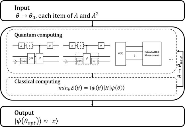
Figure 2. A schematic diagram of the entire algorithm for the one-dimensional Poisson equation with different boundary conditions. |
3.2. The d-dimensional Poisson equation with Dirichlet boundary conditions
Similarly, the d-dimensional Poisson equation with Dirichlet boundary conditions can be discretized to be the following linear system ${A}^{\left(d\right)}x=b$ , where $b\in {R}^{{n}^{d}}$ and ${A}^{\left(d\right)}\in {R}^{{n}^{d}\,\times \,{n}^{d}}$ , with
$\begin{eqnarray*}\begin{array}{rcl}{A}^{\left(d\right)} & = & A^{\prime} \otimes I\otimes ...\otimes I+I\otimes A^{\prime} \otimes I\otimes ...\\ & & \otimes I+\cdots +I\otimes \cdots \otimes I\otimes A^{\prime} \\ & = & \displaystyle \sum _{\displaystyle \genfrac{}{}{0em}{}{s=0}{s+t=d-1}}^{d-1}{I}_{s}\otimes A^{\prime} \otimes {I}_{t},\end{array}\end{eqnarray*}$
where ${I}_{s}=\mathop{\underbrace{I\otimes ...\otimes I}}\limits_{s}$ , I ∈ Rn×n.Based on the structure of $A^{\prime} $ , it can be decomposed as,
$\begin{eqnarray*}A^{\prime} =\left[\begin{array}{ccccc}2 & -1 & \cdots & 0 & 0\\ -1 & 2 & & \ddots & 0\\ \vdots & & \ddots & & \vdots \\ 0 & & & \ddots & -1\\ 0 & 0 & \cdots & -1 & 2\end{array}\right]=2I-L-{L}^{-1}+{M}_{5},\end{eqnarray*}$
where $\begin{eqnarray*}{M}_{5}=\left[\begin{array}{cccccc} & & & & & 1\\ & & & & 0 & \\ & & \ddots & & & \\ & & & \ddots & & \\ & 0 & & & & \\ 1 & & & & & \end{array}\right].\end{eqnarray*}$
For matrix M5 in ${A}^{\left(d\right)}$ , we give the following decomposition, i.e.
$\begin{eqnarray*}\begin{array}{rcl}{M}_{5} & = & \displaystyle \frac{1}{2}\left(\left[\begin{array}{cccccc} & & & & & 1\\ & & & & 1 & \\ & & \ddots & & & \\ & & & \ddots & & \\ & 1 & & & & \\ 1 & & & & & \end{array}\right]-\left[\begin{array}{cccccc} & & & & & -1\\ & & & & 1 & \\ & & \ddots & & & \\ & & & \ddots & & \\ & 1 & & & & \\ -1 & & & & & \end{array}\right]\right)\\ & = & \displaystyle \frac{1}{2}\left(\left[\begin{array}{cccccc} & & & & & 1\\ & & & & 1 & \\ & & \ddots & & & \\ & & & \ddots & & \\ & 1 & & & & \\ 1 & & & & & \end{array}\right]-\left[\begin{array}{cccccc} & & & & & 1\\ & & & & 1 & \\ & & \ddots & & & \\ & & & \ddots & & \\ & 1 & & & & \\ 1 & & & & & \end{array}\right]\left[\begin{array}{cccccc}-1 & & & & & \\ & 1 & & & & \\ & & \ddots & & & \\ & & & \ddots & & \\ & & & & 1 & \\ & & & & & -1\end{array}\right]\right)\\ & = & \displaystyle \frac{1}{2}\tilde{X}-\displaystyle \frac{1}{2}\tilde{X}\tilde{Z}.\end{array}\end{eqnarray*}$
Since M5 is contained in ${A}^{\left(d\right)}$ , we will not continue the previous calculation method. As mentioned in theorem 2 of [27], for s-sparse matrices $X\in {{\mathbb{C}}}^{{2}^{n}\times {2}^{n}}$ , there is such an algorithm in existence that, in the worst case, the number of quantum circuits required to evaluate ⟨$\Psi$∣X∣$\Psi$⟩ is 2n+1. Thus, for Is ⨂ M5 ⨂ It, the number of quantum circuits is 2Nd+1. Therefore, here we consider decomposing M5 into a linear combination of two unitary matrices, i.e. $\tilde{X}$ and $\tilde{Z}$ .
According to the above decomposition of matrix $A^{\prime} $ , we therefore obtain
$\begin{eqnarray*}\begin{array}{rcl}{A}^{\left(d\right)} & = & \displaystyle \sum _{\displaystyle \genfrac{}{}{0em}{}{s=0}{s+t=d-1}}^{d-1}{I}_{s}\otimes (2I-L-{L}^{-1}+\displaystyle \frac{1}{2}\tilde{X}-\displaystyle \frac{1}{2}\tilde{X}\tilde{Z})\otimes {I}_{t}=2{{dI}}^{\otimes d}+\displaystyle \sum _{\displaystyle \genfrac{}{}{0em}{}{s=0}{s+t=d-1}}^{d-1}{I}_{s}\otimes (-L-{L}^{-1}+\displaystyle \frac{1}{2}\tilde{X}-\displaystyle \frac{1}{2}\tilde{X}\tilde{Z})\otimes {I}_{t},\\ \langle b| {A}^{\left(d\right)}| \psi (\theta )\rangle & = & 2d\langle b| \psi (\theta )\rangle +\displaystyle \sum _{\displaystyle \genfrac{}{}{0em}{}{s=0}{s+t=d-1}}^{d-1}(-\langle b| {I}_{s}\otimes L\otimes {I}_{t}| \psi (\theta )\rangle -\langle b| {I}_{s}\otimes {L}^{-1}\otimes {I}_{t}| \psi (\theta )\rangle \\ & & +\displaystyle \frac{1}{2}\langle b| {I}_{s}\otimes \tilde{X}\otimes {I}_{t}| \psi (\theta )\rangle -\displaystyle \frac{1}{2}\langle b| {I}_{s}\otimes \tilde{X}\tilde{Z}\otimes {I}_{t}| \psi (\theta )\rangle ).\end{array}\end{eqnarray*}$
Similarly, we can obtain the decomposition of ${{A}^{\left(d\right)}}^{2}$ as
$\begin{eqnarray*}\begin{array}{rcl}{{A}^{\left(d\right)}}^{2} & = & 2\displaystyle \sum _{\displaystyle \genfrac{}{}{0em}{}{u=0,v=0}{u+v+w=d-2}}^{d-2}{I}_{u}\otimes A^{\prime} \otimes {I}_{v}\otimes A^{\prime} \otimes {I}_{w}+\displaystyle \sum _{\displaystyle \genfrac{}{}{0em}{}{s=0}{s+t=d-1}}^{d-1}{I}_{s}\otimes A{{\prime} }^{2}\otimes {I}_{t}=2\displaystyle \sum _{\displaystyle \genfrac{}{}{0em}{}{u=0,v=0}{u+v+w=d-2}}^{d-2}{I}_{u}\otimes \left(2I-L-{L}^{-1}+\displaystyle \frac{1}{2}\tilde{X}-\displaystyle \frac{1}{2}\tilde{X}\tilde{Z}\right)\otimes {I}_{v}\\ & \otimes & (2I-L-{L}^{-1}+\displaystyle \frac{1}{2}\tilde{X}-\displaystyle \frac{1}{2}\tilde{X}\tilde{Z})\otimes {I}_{w}\,+\,\displaystyle \sum _{\displaystyle \genfrac{}{}{0em}{}{s=0}{s+t=d-1}}^{d-1}{I}_{s}\otimes {\left(2I-L-{L}^{-1}+\displaystyle \frac{1}{2}\tilde{X}-\displaystyle \frac{1}{2}\tilde{X}\tilde{Z}\right)}^{2}\otimes {I}_{t}\\ & = & \left(2\cdot \displaystyle \frac{{d}^{2}-d}{2}\cdot 4I+2\displaystyle \sum _{\displaystyle \begin{array}{c}u=0,v=0\\ u+v+w=d-2\\ {U}_{1},{U}_{2}\in {{\mathscr{M}}}_{1}\end{array}}^{d-2}{I}_{u}\otimes {U}_{1}\otimes {I}_{v}\otimes {U}_{2}\otimes {I}_{w}\right)\,+\left(\displaystyle \frac{25}{4}{dI}+\displaystyle \sum _{\displaystyle \genfrac{}{}{0em}{}{s=0s+t=d-1}{{U}_{3}\in {{\mathscr{M}}}_{2}}}^{d-1}{I}_{s}\otimes {U}_{3}\otimes {I}_{t}\right)\\ & = & \left(4{d}^{2}+\displaystyle \frac{9}{4}d\right)I+2\displaystyle \sum _{\begin{array}{c}u=0,v=0\\ u+v+w=d-2\\ \displaystyle {U}_{1},{U}_{2}\in {{\mathscr{M}}}_{1}\end{array}}^{d-2}{I}_{u}\otimes {U}_{1}\otimes {I}_{v}\otimes {U}_{2}\otimes {I}_{w}+\displaystyle \sum _{\begin{array}{c}s=0\\ s+t=d-1\\ {U}_{3}\in {{\mathscr{M}}}_{2}\end{array}}^{d-1}{I}_{s}\otimes {U}_{3}\otimes {I}_{t},\\ & & \langle \psi (\theta )| {{A}^{\left(d\right)}}^{2}| \psi (\theta )\rangle =4{d}^{2}+\displaystyle \frac{9}{4}d\\ & & +2\displaystyle \sum _{\begin{array}{c}u=0,v=0\\ u+v+w=d-2\\ {U}_{1},{U}_{2}\in {{\mathscr{M}}}_{1}\end{array}}^{d-2}\langle \psi (\theta )| {I}_{u}\otimes {U}_{1}\otimes {I}_{v}\otimes {U}_{2}\otimes {I}_{w}| \psi (\theta )\rangle +\displaystyle \sum _{\begin{array}{c}s=0\\ s+t=d-1\\ {{U}}_{3}\in {{\mathscr{M}}}_{2}\end{array}}^{d-1}\langle \psi (\theta )| {I}_{s}\otimes {U}_{3}\otimes {I}_{t}| \psi (\theta )\rangle ,\end{array}\end{eqnarray*}$
where ${{\mathscr{M}}}_{1}=\{I,-L,-{L}^{-1},\tfrac{1}{2}\tilde{X},-\tfrac{1}{2}\tilde{X}\tilde{Z}\}$ and, at most, one of U1 and U2 is selected as I ∈ Rn×n, and ${{\mathscr{M}}}_{2}$ is the product of the elements of the set ${{\mathscr{M}}}_{1}$ and does not contain $I\in {R}^{{n}^{d}\times {n}^{d}}$ . In fact, ⟨$\Psi$(θ)∣Is ⨂ U3 ⨂ It∣$\Psi$(θ)⟩ only needs to compute 12 terms, i.e. $\begin{eqnarray*}\begin{array}{l}\langle \psi (\theta )| {I}_{s}\otimes {U}_{3}\otimes {I}_{t}| \psi (\theta )\rangle \\ =\,\langle \psi (\theta )| {I}_{s}\otimes (-4L-4{L}^{-1}+2\tilde{X}-\displaystyle \frac{1}{2}\tilde{Z}+{L}^{2}+{L}^{-2}\\ \ \ \ +\,\displaystyle \frac{1}{2}{\tilde{Z}}^{2}-2\tilde{X}\tilde{Z}-\displaystyle \frac{1}{2}L\tilde{X}-\displaystyle \frac{1}{2}\tilde{X}{L}^{-1}\\ -\,\displaystyle \frac{1}{2}{L}^{-1}\tilde{X}-\displaystyle \frac{1}{2}\tilde{X}L+\displaystyle \frac{1}{2}L\tilde{X}\tilde{Z}+\displaystyle \frac{1}{2}\tilde{X}\tilde{Z}{L}^{-1}\\ \ \ +\,\displaystyle \frac{1}{2}{L}^{-1}\tilde{X}\tilde{Z}+\displaystyle \frac{1}{2}\tilde{X}\tilde{Z}L)\otimes {I}_{t}| \psi (\theta )\rangle \\ =\,-4(\langle \psi (\theta )| {I}_{s}\otimes L\otimes {I}_{t}| \psi (\theta )\rangle +\overline{\langle \psi (\theta )| {I}_{s}\otimes L\otimes {I}_{t}| \psi (\theta )\rangle })\\ \ \ +\,(\langle \psi (\theta )| {I}_{s}\otimes {L}^{2}\otimes {I}_{t}| \psi (\theta )\rangle \\ \ \ +\,\overline{\langle \psi (\theta )| {I}_{s}\otimes {L}^{2}\otimes {I}_{t}| \psi (\theta )\rangle })\\ -\,\displaystyle \frac{1}{2}(\langle \psi (\theta )| {I}_{s}\otimes L\tilde{X}\otimes {I}_{t}| \psi (\theta )\rangle \\ \ \ +\,\overline{\langle \psi (\theta )| {I}_{s}\otimes L\tilde{X}\otimes {I}_{t}| \psi (\theta )\rangle })\\ -\,\displaystyle \frac{1}{2}(\langle \psi (\theta )| {I}_{s}\otimes {L}^{-1}\tilde{X}\otimes {I}_{t}| \psi (\theta )\rangle \\ \ \ +\,\overline{\langle \psi (\theta )| {I}_{s}\otimes {L}^{-1}\tilde{X}\otimes {I}_{t}| \psi (\theta )\rangle })\\ +2\langle \psi (\theta )| {I}_{s}\otimes \tilde{X}\otimes {I}_{t}| \psi (\theta )\rangle \\ \ \ -\displaystyle \frac{1}{2}(\langle \psi (\theta )| {I}_{s}\otimes \tilde{Z}\otimes {I}_{t}| \psi (\theta )\rangle \\ \ \ +\,\displaystyle \frac{1}{4}\langle \psi (\theta )| {I}_{s}\otimes {\tilde{Z}}^{2}\otimes {I}_{t}| \psi (\theta )\rangle \\ -2\langle \psi (\theta )| {I}_{s}\otimes \tilde{X}\tilde{Z}\otimes {I}_{t}| \psi (\theta )\rangle \\ \ \ +\,\displaystyle \frac{1}{2}\langle \psi (\theta )| {I}_{s}\otimes L\tilde{X}\tilde{Z}\otimes {I}_{t}| \psi (\theta )\rangle \\ \ \ +\,\displaystyle \frac{1}{2}\langle \psi (\theta )| {I}_{s}\otimes \tilde{X}\tilde{Z}{L}^{-1}\otimes {I}_{t}| \psi (\theta )\rangle \\ \ \ +\,\displaystyle \frac{1}{2}\langle \psi (\theta )| {I}_{s}\otimes {L}^{-1}\tilde{X}\tilde{Z}\otimes {I}_{t}| \psi (\theta )\rangle \\ \ \ +\,\displaystyle \frac{1}{2}\langle \psi (\theta )| {I}_{s}\otimes \tilde{X}\tilde{Z}L\otimes {I}_{t}| \psi (\theta )\rangle ,\end{array}\end{eqnarray*}$
where we use L† = L−1 in the second equation. To summarize, for the d-dimensional Poisson equation with Dirichlet boundary conditions, the number of decomposition terms of $\langle b| {A}^{\left(d\right)}| \psi (\theta )\rangle $ is 4d + 1, and the number of decomposition terms of $\langle \psi (\theta )| {{A}^{\left(d\right)}}^{2}| \psi (\theta )\rangle $ is 12d2. The computation of $\langle b| {A}^{\left(d\right)}| \psi (\theta )\rangle $ and $\langle \psi (\theta )| {{A}^{\left(d\right)}}^{2}| \psi (\theta )\rangle $ is shown in figure 3. For the d-dimensional Poisson equation with the Dirichlet boundary conditions, as in [24], the number of terms is also independent of n, and the number of decompositions is the same for $\langle b| {A}^{\left(d\right)}| \psi (\theta )\rangle $ . However, for the number of decompositions of $\langle \psi (\theta )| {{A}^{\left(d\right)}}^{2}| \psi (\theta )\rangle $ , the number of terms is much less than (4d + 1)2−(4d + 1) in [24].
Figure 3. The quantum circuits for estimating each term of $\langle b| {A}^{\left(d\right)}| \psi (\theta )\rangle $ and $\langle \psi (\theta )| {{A}^{\left(d\right)}}^{2}| \psi (\theta )\rangle $ . (a) The Hadamard test circuit to estimate each term of $\langle b| {A}^{\left(d\right)}| \psi (\theta )\rangle $ . (b) The Hadmard test circuit to estimate each term of $\langle \psi (\theta )| {{A}^{\left(d\right)}}^{2}| \psi (\theta )\rangle $ . |
3.3. Numerical simulation
We perform numerical simulation in the Python qiskit package for the one-dimensional Poisson equation with Dirichlet boundary conditions to validate the feasibility of the proposed algorithms. Via the finite-difference method, the discretized one-dimensional Poisson equation with Dirichlet boundary conditions is $A^{\prime} x=b$ . For this numerical simulation, we set $| b\rangle ={\left(\tfrac{| 0\rangle +| 1\rangle }{\sqrt{2}}\right)}^{\otimes N}$ , which can be obtained by Ub = H⨂N, i.e. ∣b⟩ = H⨂N∣0⟩, where N = 3. For the ansatz, we chose the basic hardware-efficient ansatz in the numerical simulation shown in figure 4. Since in our numerical simulation our input data contains only real elements, we choose $U({\theta }_{t}^{i})={R}_{y}({\theta }_{t}^{i})$ as a way to reduce the training parameters. Otherwise, the ansatz is generally chosen as U(θ) = Rz(αj)Ry(βj)Rz(γj).
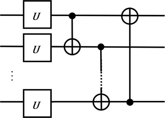
Figure 4. The basic hardware-efficient ansatz. |
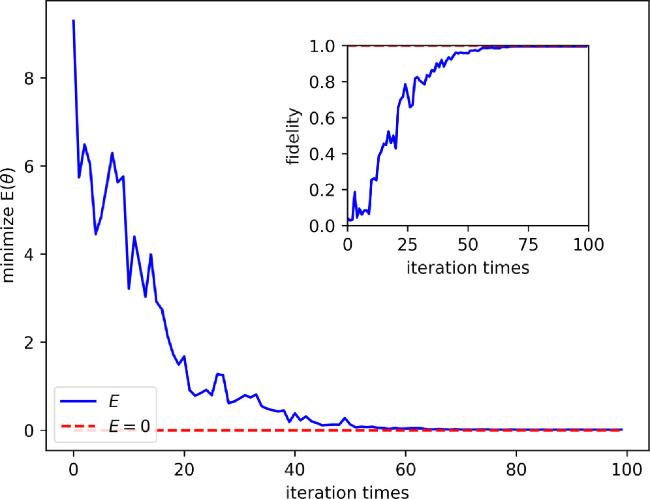
The main results are shown in figure 5, which shows the depth of the ansatz to be 2. According to figure 5, it can be seen that as the number of iteration steps increases, the value of the cost function becomes smaller. The overall trend of the fidelity ∣⟨x∣$\Psi$(θ)⟩∣ tends to 1 and the fidelity reaches more than 0.99. In addition, to avoid the cost function falling into local minimum, we solve this by choosing the parameters of [0, 2π] randomly several times.
Figure 5. The numerical simulation results of our algorithm. As the value of the cost function decreases, the value of fidelity ∣⟨x∣$\Psi$(θ)⟩∣ converges to 1. |
4. Variational algorithms for linear algebra operations with the banded Toeplitz matrix
Gao et al [28] have given an exact quantum algorithm on Toeplitz matrix-vector multiplication. In this section, we propose variational algorithms for linear algebra problems (including systems of linear equations and matrix-vector multiplication) with the K-banded Toeplitz matrix.
For a given banded Toeplitz matrix TnK, $K\in O(\mathrm{ploylog}n)$ , and an initial state vector ∣v0⟩, we can compute the normalized state
$\begin{eqnarray*}| {v}_{T}\rangle =\displaystyle \frac{{T}_{n}^{K}| {v}_{0}\rangle }{\parallel {T}_{n}^{K}| {v}_{0}\rangle \parallel },\end{eqnarray*}$
with $\parallel {T}_{n}^{K}| {v}_{0}\rangle \parallel =\langle {v}_{0}| {T}_{n}^{K\dagger }{T}_{n}^{K}| {v}_{0}\rangle $ and ${T}_{n}^{K}| {v}_{0}\rangle \ne 0$ . Here, ∣vT⟩ can be found to be the corresponding eigenstate to the Hamiltonian $\begin{eqnarray*}{H}_{T}=I-\displaystyle \frac{{T}_{n}^{K}| {v}_{0}\rangle \langle {v}_{0}| {T}_{n}^{K\dagger }}{{\parallel {T}_{n}^{K}| {v}_{0}\rangle \parallel }^{2}},\end{eqnarray*}$
with a minimum eigenvalue of 0. And we define the cost function E(θ) = ⟨$\Psi$(θ)∣HT∣$\Psi$(θ)⟩, that is, $\begin{eqnarray*}\begin{array}{rcl}\mathop{\min }\limits_{\theta }E(\theta ) & = & \mathop{\min }\limits_{\theta }\langle \psi (\theta )| {H}_{T}| \psi (\theta )\rangle \\ & = & \mathop{\min }\limits_{\theta }\langle \psi (\theta )| \Space{0ex}{2.5ex}{0ex}(I-\displaystyle \frac{{T}_{n}^{K}| {v}_{0}\rangle \langle {v}_{0}| {T}_{n}^{K\dagger }}{{\parallel {T}_{n}^{K}| {v}_{0}\rangle \parallel }^{2}}\Space{0ex}{2.5ex}{0ex})| \psi (\theta )\rangle \\ & = & 1-\mathop{\min }\limits_{\theta }\langle \psi (\theta )| \displaystyle \frac{{T}_{n}^{K}| {v}_{0}\rangle \langle {v}_{0}| {T}_{n}^{K\dagger }}{{\parallel {T}_{n}^{K}| {v}_{0}\rangle \parallel }^{2}}| \psi (\theta )\rangle \\ & = & 1-\mathop{\min }\limits_{\theta }\displaystyle \frac{| \langle \psi (\theta )| {T}_{n}^{K}| {v}_{0}\rangle {| }^{2}}{{\parallel {T}_{n}^{K}| {v}_{0}\rangle \parallel }^{2}}\\ & = & 1-\mathop{\min }\limits_{\theta }{\left|\langle \psi (\theta )| \displaystyle \frac{{T}_{n}^{K}}{\parallel {T}_{n}^{K}| {v}_{0}\rangle \parallel }| {v}_{0}\rangle \right|}^{2}\\ & = & 1-\mathop{\min }\limits_{\theta }| \langle \psi (\theta )| \tilde{{T}_{n}^{K}}| {v}_{0}\rangle {| }^{2}\\ & = & 1-\mathop{\min }\limits_{\theta }| \langle 0,\psi (\theta )| {C}_{\tilde{{T}_{n}^{K}}}| 0,{v}_{0}\rangle {| }^{2},\end{array}\end{eqnarray*}$
where $\tilde{{T}_{n}^{K}}=\tfrac{{T}_{n}^{K}}{\parallel {T}_{n}^{K}| {v}_{0}\rangle \parallel }$ and $\begin{eqnarray*}{C}_{\tilde{{T}_{n}^{K}}}=\left[\begin{array}{cc}\tilde{{T}_{n}^{K}} & B\{\tilde{{T}_{n}^{K}}\}{}_{n}\\ B\{\tilde{{T}_{n}^{K}}\}{}_{n} & \tilde{{T}_{n}^{K}}\end{array}\right].\end{eqnarray*}$
The linear system with the banded Toeplitz matrix TnK is
$\begin{eqnarray*}{T}_{n}^{K}x=b.\end{eqnarray*}$
We also transform the problem of solving the linear system to find the ground state of a Hamiltonian, $H\,={{T}_{n}^{K}}^{\dagger }(I-| b\rangle \langle b| ){T}_{n}^{K}$ , where $\left|b\right\rangle \propto b$ . And we assume that there is an efficient unitary operator Ub that can prepare a quantum state $\left|b\right\rangle $ . Therefore, the cost function can be expressed as
$\begin{eqnarray*}\begin{array}{rcl}\mathop{\min }\limits_{\theta }E(\theta ) & = & \mathop{\min }\limits_{\theta }\langle \psi (\theta )| H| \psi (\theta )\rangle \\ & = & \mathop{\min }\limits_{\theta }[\langle \psi (\theta )| {{T}_{n}^{K}}^{2}| \psi (\theta )\rangle -{\left|\langle b| {T}_{n}^{K}| \psi (\theta )\rangle \right|}^{2}]\\ & = & \mathop{\min }\limits_{\theta }[\langle 0,\psi (\theta )| {C}_{{{T}_{n}^{K}}^{2}}| 0,\psi (\theta )\rangle \\ & & -{\left|\langle 0,b| {C}_{{T}_{n}^{K}}| 0,\psi (\theta )\rangle \right|}^{2}],\end{array}\end{eqnarray*}$
where $\begin{eqnarray*}{C}_{{{T}_{n}^{K}}^{2}}=\left[\begin{array}{cc}{{T}_{n}^{K}}^{2} & B{\{{{T}_{n}^{K}}^{2}\}}_{n}\\ B{\{{{T}_{n}^{K}}^{2}\}}_{n} & {{T}_{n}^{K}}^{2}\end{array}\right],\end{eqnarray*}$
and $\begin{eqnarray*}{C}_{{T}_{n}^{K}}=\left[\begin{array}{cc}{T}_{n}^{K} & B\{{T}_{n}^{K}\}{}_{n}\\ B\{{T}_{n}^{K}\}{}_{n} & {T}_{n}^{K}\end{array}\right].\end{eqnarray*}$
The estimation of the cost function involved in this section can be obtained from the previous quantum circuits. Thus, equations such as the heat equation, Poisson equation and other equations involved in engineering, when discretized, can be transformed into a linear system with the banded Toeplitz matrix solved and combined with the extended Bell measurements.
5. Conclusion
In this paper, we focus on solving the one-dimensional Poisson equation with different boundary conditions and the d-dimensional Poisson equation with Dirichlet boundary conditions on NISQ devices and further give the VQAs for linear algebra with the banded Toeplitz matrix. As in general linear system solutions, we transform the solution of the discretized Poisson equation into a problem of solving its ground state in terms of the Hamiltonian associated with the coefficient matrix A, and we use the structural features of A and A2 to efficiently evaluate the value of the cost function. In detail, we use the structural features of the matrices A and A2 to decompose into a linear combination of the banded Toeplitz matrices and a few sparse matrices. Then, for the one-dimensional Poisson equation with different boundary conditions and the d-dimensional Poisson equation with Dirichlet boundary conditions, the number of terms to decompose $\langle b| \tilde{A}| \psi (\theta )\rangle $ and $\langle b| {A}^{\left(d\right)}| \psi (\theta )\rangle $ is 5 and 4d + 1 respectively, and the number of terms to decompose $\langle \psi (\theta )| {\tilde{A}}^{2}| \psi (\theta )\rangle $ and $\langle \psi (\theta )| {{A}^{\left(d\right)}}^{2}| \psi (\theta )\rangle $ is 6 and 12d2, respectively. The quantum circuit consists of two main parts, one of which is the Hadamard test and the other is the extended Bell measurement. Using the Hadamard test to estimate the values (e.g. figure 1(a) and (b)) has a complexity of O((N + 1)2) due to the due to the Quantum Fourier Transform (QFT), and the depth of the QFT can also be reduced to O(N) [29]. The quantum circuits require only two ancillary qubits, one of which is needed to extend the A to the circulant matrix, and the other is needed for the Hadamard test. Moreover, for estimating $\langle 0,\psi (\theta )| {F}_{n}^{-1}{D}^{l}{F}_{n}| 0,\psi (\theta )\rangle $ , figure 1(b) can also be solved using the generalized swap-test circuit, as mentioned in [30]. More importantly, our algorithm only requires changing the part of the circuit D involving the parameters for estimating $\langle 0,\psi (\theta )| {F}_{n}^{-1}{D}^{l}{F}_{n}| 0,\psi (\theta )\rangle $ . The complexity of estimating Mi using the extended Bell measurement method is, at most, O(N) and does not require ancillary qubits. Finally, the quantum circuits have been explicitly constructed to efficiently evaluate the value of the cost function.
We emphasis that our algorithm for evaluating the cost function is very efficient since the number of decomposition terms is only polynomial of d and independent of n. As a result, our algorithm greatly reduces the number of measurements compared to the algorithm in [21]. Like the algorithm in [24], our approach does not depend on the size of the dimension n of the linear system. Furthermore, we reduce the number of decomposition terms and provide the simpler circuit construction. In this paper, VQAs for linear systems with Toeplitz matrices are proposed, which are adapted for Hermitian and sparse coefficient matrices satisfying ai,i+c = ac, for all c = 0, 1, ⋯ ,n − 1 and i = 0, ⋯ ,n − 1 − c, where ai,i+c denotes the element of the coefficient matrices mentioned in [24].
Acknowledgments
This work is supported by the Shandong Provincial Natural Science Foundation for Quantum Science under Grant No. ZR2021LLZ002 and the Fundamental Research Funds for the Central Universities under Grant No. 22CX03005A.