


1. Introduction
The physical behaviors of nanostructures are interesting and have potential applications in engineering science. Among the nanostructures, quantum dots (QDs) and quantum rings (QRs) have received much attention. The study of thermodynamic and magnetic properties of QDs and QRs are important challenges in the science of physics [1–7].
The confinement potentials have a crucial role in investigating the thermodynamic and magnetic properties of quantum dot/ring systems. The available confinement potentials such as the Fu–Wang–Jia potential [8, 9] and its special cases also have a substantial role in the accurate prediction of thermodynamic properties for real substance systems and the successful prediction of equilibrium constants for some important chemical reactions [10–14].
In past years, many researchers have tried to study the physical properties of nanostructures analytically [15–19]. Also, many authors have tried to investigate the effects of electron–electron (e–e) interaction, magnetic field, and spin–orbit interaction (SOI) on the physical properties of QDs and QRs [20–25]. As we know, analytical study is very valuable. Although, due to the complicated form of the e–e interaction and SOI, the analytical study of the physical properties of nanostructures requires considerable theoretical effort. The reader can refer to [26–28].
One of the most important physical properties of nanostructures are the magnetic properties. Hitherto, many papers have reported on the magnetic properties of QDs and QRs [29–34]. Recently, Shi et al [35] investigated dynamic magnetic properties and the magnetocaloric effect of a decorated square structure. It is to be noted that the magnetic properties of QDs and QRs change under various factors like SOI, impurity, e–e interaction, and magnetic field. Several articles have reported on the magnetic properties of QDs under Rashba SOI and e–e interaction [29–32, 36–40].
According to the importance of the subject, we have tried to study the magnetic properties of a quantum dot/ring system under a magnetic field, e–e interaction, and Rashba SOI. To reach this goal, we analytically solve the Schrödinger equation and obtain the electron energy levels. Then, we determine magnetization, and magnetic susceptibility under the aforementioned factors.
2. Theory and model
Consider a dot/ring system with two electrons under an external magnetic field $B,$ and the Rashba SOI. The total Hamiltonian of the system is expressed as:
$\begin{eqnarray}H={H}_{0}+{H}_{R}+\displaystyle \frac{{e}^{2}}{\left|{{\boldsymbol{r}}}_{2}-{{\boldsymbol{r}}}_{1}\right|}+{H}_{Z}.\end{eqnarray}$
The first term $\left({H}_{0}\right)$ is the Hamiltonian of two electrons without the e–e interaction and the Rashba effect. The second term is the Rashba Hamiltonian, the third term is the e–e interaction, and the fourth term is the Zeeman Hamiltonian. The Hamiltonian of ${H}_{0}$ is given by $\begin{eqnarray}{H}_{0}=\displaystyle \frac{1}{2{m}^{\ast }}\displaystyle \sum _{j=1}^{2}{\left({{\boldsymbol{P}}}_{j}+e{{\boldsymbol{A}}}_{j}\right)}^{2}+V\left({{\boldsymbol{r}}}_{1},{{\boldsymbol{r}}}_{2}\right),\end{eqnarray}$
where ${m}^{* }$ is the electron effective mass, and ${{\boldsymbol{A}}}_{j}\,=\tfrac{B}{2}\left(-{y}_{j},{x}_{j},0\right)=\tfrac{B{r}_{j}}{2}{\boldsymbol{\varphi }}$ is the vector potential. Also, $V\left({{\boldsymbol{r}}}_{1},{{\boldsymbol{r}}}_{2}\right)$ is the confining potential with two terms, a parabolic-inverse square (PIS), and a Gaussian term. One can write $V\left({{\boldsymbol{r}}}_{1},{{\boldsymbol{r}}}_{2}\right)={V}_{1}\left({{\boldsymbol{r}}}_{1},{{\boldsymbol{r}}}_{2}\right)+{V}_{2}\left({{\boldsymbol{r}}}_{1},{{\boldsymbol{r}}}_{2}\right).$ The PIS potential is written as [29],3 ) and (5 ), we have:
$\begin{eqnarray}{V}_{1}\left({{\boldsymbol{r}}}_{1},{{\boldsymbol{r}}}_{2}\right)=\displaystyle \frac{1}{2}{m}^{\ast }{\omega }_{0}^{2}{\left|{{\boldsymbol{r}}}_{2}-{{\boldsymbol{r}}}_{1}\right|}^{2}+\displaystyle \frac{{\hslash }^{2}\xi }{2{m}^{\ast }}\displaystyle \frac{1}{{\left|{{\boldsymbol{r}}}_{2}-{{\boldsymbol{r}}}_{1}\right|}^{2}},\end{eqnarray}$
where ${\omega }_{0}$ is the harmonic frequency, and $\xi $ is a dimensionless parameter. The Gaussian potential is written as: $\begin{eqnarray}{V}_{2}\left({{\boldsymbol{r}}}_{1},{{\boldsymbol{r}}}_{2}\right)=-{V}_{0}\exp \left[-{\left(\displaystyle \frac{\left|{{\boldsymbol{r}}}_{2}-{{\boldsymbol{r}}}_{1}\right|}{{R}_{0}}\right)}^{q}\right],\end{eqnarray}$
where ${V}_{0}$ and ${R}_{0}$ are the depth and range of the potential. We suppose that $q=2$ and $r/{R}_{0}\ll 1,$ hence the Gaussian potential can be expressed by: $\begin{eqnarray}{V}_{2}\left({{\boldsymbol{r}}}_{1},{{\boldsymbol{r}}}_{2}\right)=-\left({V}_{0}-\displaystyle \frac{{V}_{0}}{{R}_{0}^{2}}{\left|{{\boldsymbol{r}}}_{2}-{{\boldsymbol{r}}}_{1}\right|}^{2}\right).\end{eqnarray}$
Combining equations ( $\begin{eqnarray}\begin{array}{c}V\left({{\boldsymbol{r}}}_{1},{{\boldsymbol{r}}}_{2}\right)=-{V}_{0}\\ \,+\,\left(\displaystyle \frac{1}{2}{m}^{\ast }{\omega }_{0}^{2}+\displaystyle \frac{{V}_{0}}{{R}_{0}^{2}}\right){\left|{{\boldsymbol{r}}}_{2}-{{\boldsymbol{r}}}_{1}\right|}^{2}+\displaystyle \frac{{\hslash }^{2}\xi }{2{m}^{\ast }}\displaystyle \frac{1}{{\left|{{\boldsymbol{r}}}_{2}-{{\boldsymbol{r}}}_{1}\right|}^{2}}.\end{array}\end{eqnarray}$
The Rashba Hamiltonian is given by $\begin{eqnarray}{H}_{R}=\displaystyle \frac{{\alpha }_{R}}{\hslash }\displaystyle \sum _{j=1}^{2}\left[{{\boldsymbol{\sigma }}}_{j}\times \left({{\boldsymbol{P}}}_{j}+e{{\boldsymbol{A}}}_{j}\right)\right].\end{eqnarray}$
Here, ${\alpha }_{R}$ is the Rashba coupling parameter, and $\sigma \,=\left({\sigma }_{x},{\sigma }_{y},{\sigma }_{z}\right)$ are the Pauli matrices. The Zeeman term is given by $\begin{eqnarray}{H}_{Z}=\displaystyle \frac{1}{2}{g}^{\ast }{\mu }_{B}B\displaystyle \sum _{j=1}^{2}{\sigma }_{j,z},\end{eqnarray}$
where ${g}^{* }$ is the Landé factor of the electron, and ${\mu }_{B}$ is the Bohr magneton.We employ the Jacobi coordinates [33, 35] as follows:8 )–(14 ), the total Hamiltonian is separated into the center of mass and relative coordinate parts, $H={H}_{r}+{H}_{R}.$ 15 ), consider the wave function as ${\rm{\Phi }}\left(r,\theta \right)\,=\tfrac{{{\rm{e}}}^{{\rm{i}}m\theta }}{\sqrt{2\pi }}f\left(r\right),$ and obtain:17 ), we have:19 ), the following equations can be obtained:
$\begin{eqnarray}\begin{array}{c}{\boldsymbol{R}}=\displaystyle \frac{{{\boldsymbol{r}}}_{1}+{{\boldsymbol{r}}}_{2}}{2},\,{\boldsymbol{r}}=\,{{\boldsymbol{r}}}_{2}-{{\boldsymbol{r}}}_{1},\,\\ {{\boldsymbol{P}}}_{R}={{\boldsymbol{P}}}_{1}+{{\boldsymbol{P}}}_{2},\,{{\boldsymbol{P}}}_{r}=\displaystyle \frac{{{\boldsymbol{P}}}_{2}-{{\boldsymbol{P}}}_{1}}{2}.\end{array}\end{eqnarray}$
Therefore, we obtain the following relations: $\begin{eqnarray}\begin{array}{c}\displaystyle \frac{1}{2{m}^{\ast }}\displaystyle \sum _{j=1}^{2}{\left({{\boldsymbol{P}}}_{j}+e{{\boldsymbol{A}}}_{j}\right)}^{2}=\,\displaystyle \frac{{{P}_{R}}^{2}}{2M}+\displaystyle \frac{{{P}_{r}}^{2}}{2\mu }+\displaystyle \frac{1}{2}{\omega }_{c}{l}_{zR}\\ \,+\,\displaystyle \frac{1}{2}{\omega }_{c}{l}_{zr}+\displaystyle \frac{1}{8}M{\omega }_{c}^{2}{R}^{2}+\displaystyle \frac{1}{8}\mu {\omega }_{c}^{2}{r}^{2},\end{array}\end{eqnarray}$
$\begin{eqnarray}\begin{array}{c}V\left({{\boldsymbol{r}}}_{1},{{\boldsymbol{r}}}_{2}\right)=-{V}_{0}\\ \,+\,\left(\displaystyle \frac{1}{2}{m}^{\ast }{\omega }_{0}^{2}+\displaystyle \frac{{V}_{0}}{{R}_{0}^{2}}\right){r}^{2}+\displaystyle \frac{{\hslash }^{2}\xi }{2{m}^{* }}\displaystyle \frac{1}{{r}^{2}},\end{array}\end{eqnarray}$
$\begin{eqnarray}\begin{array}{c}{H}_{R}=\displaystyle \frac{{\alpha }_{R}}{\hslash }\displaystyle \sum _{j=1}^{3}\left[{\sigma }_{x}^{\left(j\right)}\left({P}_{y}^{\left(j\right)}+e{A}_{y}^{\left(j\right)}\right)-{\sigma }_{y}^{\left(j\right)}\left({P}_{x}^{\left(j\right)}+e{A}_{x}^{\left(j\right)}\right)\right]\\ \,=\,\displaystyle \frac{{\alpha }_{R}}{\hslash }\left(\begin{array}{cc}0 & {H}_{12}^{R}\\ {H}_{21}^{R} & 0\end{array}\right),\end{array}\end{eqnarray}$
where $\begin{eqnarray}\begin{array}{c}{H}_{12}^{R}=\displaystyle \sum _{j=1}^{2}\left[\displaystyle \frac{\hslash }{{\rm{i}}}\left(\displaystyle \frac{\partial }{\partial {y}_{j}}+{\rm{i}}\displaystyle \frac{\partial }{\partial {x}_{j}}\right)+\displaystyle \frac{eB}{2}\left({x}_{j}-{\rm{i}}{y}_{j}\right)\right]\\ \,=\,\displaystyle \frac{\hslash }{{\rm{i}}}\left(\displaystyle \frac{\partial }{\partial {R}_{y}}+{\rm{i}}\displaystyle \frac{\partial }{\partial {R}_{x}}\right)+eB\left({R}_{x}-{\rm{i}}{R}_{y}\right),\end{array}\end{eqnarray}$
$\begin{eqnarray}\begin{array}{c}{H}_{21}^{R}=\displaystyle \sum _{j=1}^{2}\left[\displaystyle \frac{\hslash }{{\rm{i}}}\left(\displaystyle \frac{\partial }{\partial {y}_{j}}-{\rm{i}}\displaystyle \frac{\partial }{\partial {x}_{j}}\right)+\displaystyle \frac{eB}{2}\left({x}_{j}+{\rm{i}}{y}_{j}\right)\right]\\ \,=\,\displaystyle \frac{\hslash }{{\rm{i}}}\left(\displaystyle \frac{\partial }{\partial {R}_{y}}-{\rm{i}}\displaystyle \frac{\partial }{\partial {R}_{x}}\right)+eB\left({R}_{x}+{\rm{i}}{R}_{y}\right).\end{array}\end{eqnarray}$
According to equations ( $\begin{eqnarray}\begin{array}{c}{H}_{r}{\rm{\Phi }}=-\displaystyle \frac{{\hslash }^{2}}{2\mu }\left[\displaystyle \frac{{{\rm{d}}}^{2}}{{\rm{d}}{r}^{2}}+\displaystyle \frac{1}{r}\displaystyle \frac{{\rm{d}}}{{\rm{d}}r}+\displaystyle \frac{1}{{r}^{2}}\displaystyle \frac{{{\rm{d}}}^{2}}{{\rm{d}}{\theta }^{2}}\right]{\rm{\Phi }}\\ \,+\,\displaystyle \frac{1}{2}{\omega }_{c}{l}_{zr}{\rm{\Phi }}+\displaystyle \frac{{e}^{2}}{r}{\rm{\Phi }}+\displaystyle \frac{{\hslash }^{2}\xi }{2\mu }\displaystyle \frac{1}{{r}^{2}}{\rm{\Phi }}\\ \,-\,{V}_{0}{\rm{\Phi }}+\displaystyle \frac{1}{2}\mu {{\rm{\Omega }}}^{2}{r}^{2}{\rm{\Phi }}={E}_{r}{\rm{\Phi }},\end{array}\end{eqnarray}$
where ${{\rm{\Omega }}}^{2}=\tfrac{{\omega }_{c}^{2}}{4}+{\omega }_{0}^{2}+\tfrac{2{V}_{0}}{\mu {R}_{0}^{2}}.$ $\begin{eqnarray*}\begin{array}{l}{H}_{R}{\rm{\Psi }}=-\displaystyle \frac{{\hslash }^{2}}{2M}\left[\displaystyle \frac{{\partial }^{2}}{\partial {R}_{x}^{2}}+\displaystyle \frac{{\partial }^{2}}{\partial {R}_{y}^{2}}\right]{\rm{\Psi }}+\displaystyle \frac{1}{2}{\omega }_{c}{l}_{zR}{\rm{\Psi }}\\ \,+\,\displaystyle \frac{1}{8}M{\omega }_{c}^{2}{R}^{2}{\rm{\Psi }}+\left(\begin{array}{cc}\displaystyle \frac{1}{2}{g}^{\ast }{\mu }_{B}B & 0\\ 0 & -\displaystyle \frac{1}{2}{g}^{\ast }{\mu }_{B}B\end{array}\right){\rm{\Psi }}\end{array}\end{eqnarray*}$
$\begin{eqnarray}+\,\displaystyle \frac{{\alpha }_{R}}{\hslash }\left(\begin{array}{cc}0 & {H}_{12}^{R}\\ {H}_{21}^{R} & 0\end{array}\right){\rm{\Psi }}={E}_{R}{\rm{\Psi }}.\end{eqnarray}$
To solve equation ( $\begin{eqnarray}\begin{array}{c}\displaystyle \frac{{{\rm{d}}}^{2}f}{{\rm{d}}{r}^{2}}+\displaystyle \frac{1}{r}\displaystyle \frac{{\rm{d}}f}{{\rm{d}}r}-\displaystyle \frac{{m}^{2}+\xi }{{r}^{2}}f\\ \,-\,\displaystyle \frac{2\mu }{{\hslash }^{2}}\left[\displaystyle \frac{1}{2}\mu {{\rm{\Omega }}}^{2}{r}^{2}+\displaystyle \frac{{e}^{2}}{r}-{V}_{0}-\displaystyle \frac{m\hslash }{2}{\omega }_{c}-{E}_{r}\right]f=0.\end{array}\end{eqnarray}$
Here, we define the following notations: $\begin{eqnarray}\begin{array}{c}\displaystyle \frac{2\mu \left({E}_{r}+{V}_{0}\right)}{{\hslash }^{2}}+\displaystyle \frac{m\mu {\omega }_{c}}{\hslash }=\,{\varepsilon }_{r},\,\displaystyle \frac{{\mu }^{2}{{\rm{\Omega }}}^{2}}{{\hslash }^{2}}={\lambda }^{2},\,\displaystyle \frac{2\mu {e}^{2}}{{\hslash }^{2}}=\eta .\end{array}\end{eqnarray}$
Considering the radial wave function as $f\left(r\right)\,={{\rm{e}}}^{-c{r}^{2}-dr}\displaystyle \displaystyle \sum _{n}{a}_{n}{r}^{n+k}$ where $\gamma ,$ and $\delta $ are constant. Inserting $f\left(r\right)$ into equation ( $\begin{eqnarray}\begin{array}{c}\displaystyle \displaystyle \sum _{n=0}{a}_{n}\left[\left(n+k\right)\left(n+k-1\right)+\left(n+k\right)-\left({m}^{2}+\xi \right)\right]{r}^{n+k-2}\\ \,+\,\displaystyle \displaystyle \sum _{n=0}{a}_{n}\left[-2d\left(n+k\right)-\eta -d\right]{r}^{n+k-1}\\ \,+\,\displaystyle \displaystyle \sum _{n=0}{a}_{n}\left[-4c\left(n+k\right)+{d}^{2}-4c+{\varepsilon }_{r}\right]{r}^{n+k}\\ \,+\,\displaystyle \displaystyle \sum _{n=0}{a}_{n}\left[4cd\right]{r}^{n+k+1}+\displaystyle \sum _{n=0}{a}_{n}\left[4{c}^{2}-{\lambda }^{2}\right]{r}^{n+k+2}=0.\end{array}\end{eqnarray}$
According to equation ( $\begin{eqnarray}{k}^{2}={m}^{2}+\xi ,\,{\varepsilon }_{r}=4c\left(n+k\right)-{d}^{2}+4c,\end{eqnarray}$
$\begin{eqnarray}4{c}^{2}-{\lambda }^{2}=0,\,2d\left(n+k\right)+\eta +d=0.\end{eqnarray}$
Using equations (18 ), (20 ), and (21 ), we get the following energy eigenvalues:16 ) can be written as:25 ), one has:26 ) and (27 ), the following solutions are considered,30 ) and (31 ) into (26 ) and (27 ). Then, using the recurrence relations, and Bessel differential equation, the energy levels ${E}_{R}$ of the system can be obtained.
$\begin{eqnarray}\begin{array}{c}{E}_{r}=\hslash {\rm{\Omega }}\left(n+1+\sqrt{{m}^{2}+\xi }\right)\\ \,-\,\displaystyle \frac{2\mu {e}^{4}}{{\hslash }^{2}{\left(2n+1+2\sqrt{{m}^{2}+\xi }\right)}^{2}}+\displaystyle \frac{1}{2}m\hslash {\omega }_{c}-{V}_{0}.\end{array}\end{eqnarray}$
Now, equation ( $\begin{eqnarray*}\begin{array}{c}-\displaystyle \frac{{\hslash }^{2}}{2M}\left[\displaystyle \frac{{\partial }^{2}}{\partial {R}_{x}^{2}}+\displaystyle \frac{{\partial }^{2}}{\partial {R}_{y}^{2}}\right]{\rm{\Psi }}+\displaystyle \frac{1}{2}{\omega }_{c}{l}_{zR}{\rm{\Psi }}\\ +\,\displaystyle \frac{1}{8}M{\omega }_{c}^{2}{R}^{2}{\rm{\Psi }}+\left(\begin{array}{cc}\displaystyle \frac{1}{2}{g}^{\ast }{\mu }_{B}B & 0\\ 0 & -\displaystyle \frac{1}{2}{g}^{\ast }{\mu }_{B}B\end{array}\right){\rm{\Psi }}\end{array}\end{eqnarray*}$
$\begin{eqnarray}+\,\displaystyle \frac{{\alpha }_{R}}{\hslash }\left(\begin{array}{cc}0 & {H}_{12}^{R}\\ {H}_{21}^{R} & 0\end{array}\right){\rm{\Psi }}={E}_{R}{\rm{\Psi }}.\end{eqnarray}$
Choosing ${R}_{x}=R\,\cos \,\phi ,$ ${R}_{y}=R\,\sin \,\phi ,$ and $R=\sqrt{{R}_{x}^{2}+{R}_{y}^{2}},$ we have: $\begin{eqnarray}\begin{array}{c}\displaystyle \frac{\partial }{\partial {R}_{x}}=\,\cos \,\phi \displaystyle \frac{\partial }{\partial R}-\displaystyle \frac{\sin \,\phi }{R}\displaystyle \frac{\partial }{\partial \phi },\\ \displaystyle \frac{\partial }{\partial {R}_{y}}=\,\sin \,\phi \displaystyle \frac{\partial }{\partial R}+\displaystyle \frac{\cos \,\phi }{R}\displaystyle \frac{\partial }{\partial \phi }.\end{array}\end{eqnarray}$
Using the above equation, we can write: $\begin{eqnarray}\begin{array}{c}{H}_{12}^{R}=\displaystyle \frac{\hslash }{{\rm{i}}}{{e}}^{-{\rm{i}}\phi }\left[{\rm{i}}\displaystyle \frac{\partial }{\partial R}+\displaystyle \frac{1}{R}\displaystyle \frac{\partial }{\partial \phi }\right]+{e}BR{{e}}^{-{\rm{i}}\phi },\\ {H}_{21}^{R}=\displaystyle \frac{\hslash }{{\rm{i}}}{{e}}^{{\rm{i}}\phi }\left[-{\rm{i}}\displaystyle \frac{\partial }{\partial R}+\displaystyle \frac{1}{R}\displaystyle \frac{\partial }{\partial \phi }\right]+{e}BR{{\rm{e}}}^{{\rm{i}}\phi }.\end{array}\end{eqnarray}$
Considering ${\rm{\Psi }}=\left(\begin{array}{c}u\left(R\right){{\rm{e}}}^{{\rm{i}}m\phi }\\ v\left(R\right){{\rm{e}}}^{{\rm{i}}\left(m+1\right)\phi }\end{array}\right)$ and inserting it into equation ( $\begin{eqnarray*}\begin{array}{c}\displaystyle \frac{{{\rm{d}}}^{2}u}{{\rm{d}}{R}^{2}}+\displaystyle \frac{1}{R}\displaystyle \frac{{\rm{d}}u}{{\rm{d}}R}+\left({k}^{2}-\displaystyle \frac{{m}^{2}}{{R}^{2}}\right)u\\ \,-\,\displaystyle \frac{{\omega }_{c}^{2}}{4{\hslash }^{2}}{R}^{2}u-\displaystyle \frac{2M{\alpha }_{R}}{\hslash }\left(\displaystyle \frac{{\rm{d}}}{{\rm{d}}R}+\displaystyle \frac{m+1}{R}\right)v\end{array}\end{eqnarray*}$
$\begin{eqnarray}-\,\displaystyle \frac{2M{\alpha }_{R}eB}{\hslash }Rv=0,\,\end{eqnarray}$
$\begin{eqnarray*}\displaystyle \frac{{{\rm{d}}}^{2}v}{{\rm{d}}{R}^{2}}+\displaystyle \frac{1}{R}\displaystyle \frac{{\rm{d}}v}{{\rm{d}}R}+\left({q}^{2}-\displaystyle \frac{{\left(m+1\right)}^{2}}{{R}^{2}}\right)v-\displaystyle \frac{{\omega }_{c}^{2}}{4{\hslash }^{2}}{R}^{2}v\,\end{eqnarray*}$
$\begin{eqnarray}\,-\,\displaystyle \frac{2M{\alpha }_{R}}{\hslash }\left(-\displaystyle \frac{{\rm{d}}}{{\rm{d}}R}+\displaystyle \frac{m}{R}\right)u-\displaystyle \frac{2M{\alpha }_{R}{e}B}{\hslash }Ru=0,\end{eqnarray}$
where, $\begin{eqnarray}{k}^{2}=-\displaystyle \frac{Mm{\omega }_{c}}{\hslash }-\displaystyle \frac{M{g}^{\ast }{\mu }_{B}B}{{\hslash }^{2}}+\displaystyle \frac{2M{E}_{R}}{{\hslash }^{2}},\end{eqnarray}$
$\begin{eqnarray}{q}^{2}=-\displaystyle \frac{M\left(m+1\right){\omega }_{c}}{\hslash }+\displaystyle \frac{M{g}^{\ast }{\mu }_{B}B}{{\hslash }^{2}}+\displaystyle \frac{2M{E}_{R}}{{\hslash }^{2}}.\end{eqnarray}$
To solve equations ( $\begin{eqnarray}u=A{{\rm{J}}}_{m}\left(kR\right)+B{{\rm{J}}}_{m}\left(qR\right),\end{eqnarray}$
$\begin{eqnarray}v=A{{\rm{J}}}_{m+1}\left(kR\right)+B{{\rm{J}}}_{m+1}\left(qR\right).\end{eqnarray}$
Inserting equations (2.1. Susceptibility and magnetization
The partition function is expressed by,
$\begin{eqnarray}Z=\displaystyle \displaystyle \sum _{s}{{\rm{e}}}^{-\beta {E}_{s}},\end{eqnarray}$
where ${E}_{s}$ is the energy eigenvalue, $\beta =1/{k}_{B}T,$ and ${k}_{{\rm{B}}}$ is Boltzmann’s constant. The magnetization, and susceptibility are given by, $\begin{eqnarray}M=\displaystyle \frac{1}{Z}\displaystyle \displaystyle \sum _{s}\left(-\displaystyle \frac{\partial {E}_{s}}{\partial B}\right){{\rm{e}}}^{-\beta {E}_{s}},\end{eqnarray}$
$\begin{eqnarray}\chi =\displaystyle \frac{1}{Z}\displaystyle \displaystyle \sum _{s}\left(-\displaystyle \frac{{\partial }^{2}{E}_{s}}{\partial {B}^{2}}\right){{\rm{e}}}^{-\beta {E}_{s}}.\end{eqnarray}$
3. Numerical results
We have chosen GaAs to show the numerical results. The following parameters have been employed: ${m}^{\ast }=0.067\,{m}_{0},$ ${g}^{\ast }=-0.44,$ ${\alpha }_{R}$ = 5.4 meV-nm, $\hslash {\omega }_{0}$ = 0.019 meV, and ${V}_{0}$ = 300 meV.
In figure 1(a), a schematic of the quantum dot/quantum ring (QD/QR) structure is shown. This system is composed of a QD separated from a surrounding concentric QR by a tunneling barrier ${V}_{0}.$ Figure 1(b) displays the curve of the actual single-particle potential energy as a function of distance with arbitrary values [32].
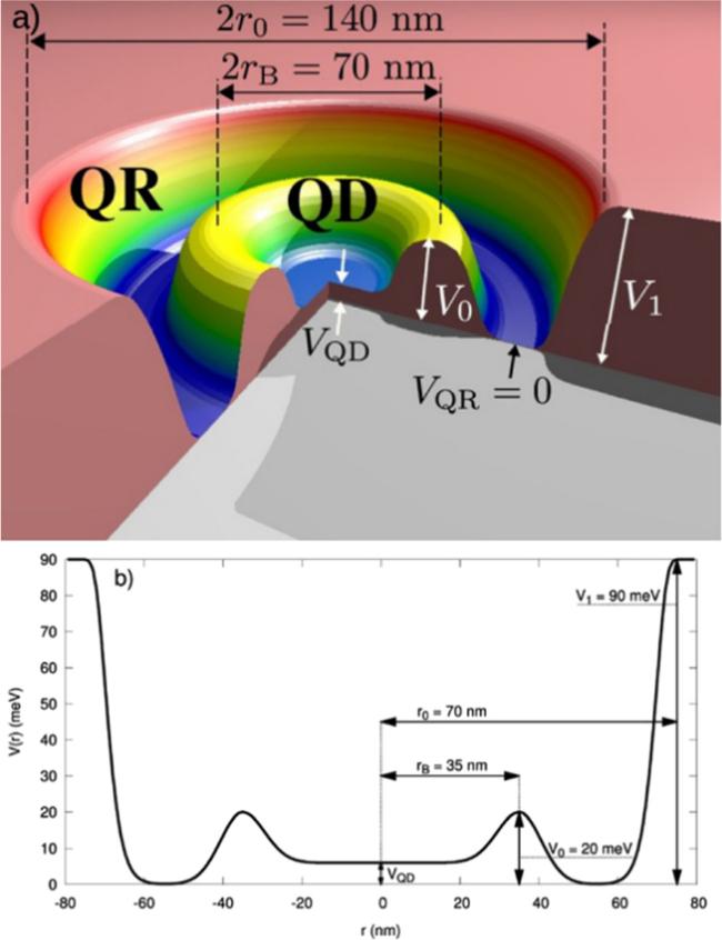
Figure 1. Schematic diagram of QD/QR structure; (b) the shape of the actual single-particle potential energy, with arbitrary values. |
Figure 2 displays the reduced energy $\left(E/\hslash {\omega }_{0}\right)$ of the two-electron system versus the magnetic field, and without Rashba SOI. Two curves correspond to the ground and first excited states. We know that in the absence of a magnetic field, the energy levels of various states within an atomic orbital are identical. If a magnetic field is applied, the states split according to the Zeeman effect and take a great variety of values. The amount of splitting is entirely dependent on the strength of the field applied. As can be seen, the energy increases as the magnetic field enhances. In the absence of Rashba effect, as the magnetic field increases, the system receives more energy and the energy values increase. According to the obtained relations, the energy of the system depends on the magnetic field value. We can see from figure 2 that a singlet → triplet transition at a critical value of ${B}_{c}$ in the presence of e–e interaction.
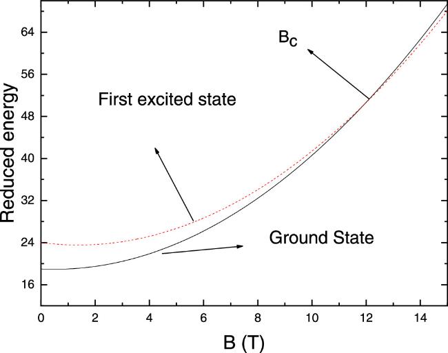
Figure 2. Reduced energy $\left(E/\hslash {\omega }_{0}\right)$ versus the magnetic field with e–e interaction and without SOI. |
Figure 3 demonstrates reduced magnetization $\left(M/{\mu }_{B}^{* }\right)$ of the two-electron system versus reduced magnetic field $\left({\omega }_{0}/{\omega }_{c}\right)$ without the e–e interaction at $T=1\,{\rm{K}}.$ The plotted curves correspond to the presence and absence of Rashba SOI. It can be seen that the magnetization increases by enhancing $B$ without and with SOI. We know that at low temperatures ($T=1\,{\rm{K}}$ ), only the lower energy states are more likely to be occupied. From the figure, it is observed that the SOI slightly modifies the magnetization of the system. When $B$ rises, the degeneracy is lifted due to the influence of the field on the Landau level and Zeeman splitting.
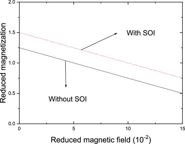
Figure 3. Reduced magnetization $\left(M/{\mu }_{B}^{* }\right)$ versus the reduced magnetic field $\left({\omega }_{0}/{\omega }_{c}\right)$ without e–e interaction with T = 1 K. |
In figure 4, the susceptibility is plotted versus $B$ for different temperatures with and without e–e interaction. As can be seen, the susceptibility rises by increasing the magnetic field, and it has a peak structure. The susceptibility reduces with rising temperature because the system disorder increases. In the presence of e–e interaction, the maximum value of the curve moves to lower magnetic fields. By considering e–e interaction, the system receives more addition energy (third term in equation (1 )). When the susceptibility reaches a maximum, the system disorder decreases. We see also the width and height of the plotted curves depend on the temperature. In the absence of SOI, the system order depends on temperature, magnetic field, and e–e interaction. There is a competition between three factors. Since the used temperatures are low, the main competition is between e–e interaction and magnetic field.
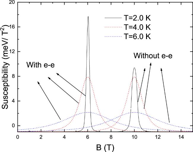
Figure 4. The susceptibility versus the magnetic field without SOI. |
Figure 5 presents the susceptibility versus temperature without and with e–e interaction for $B$ = 0.5 T. As can be seen, the susceptibility rises by increasing the temperature without and with e–e interaction. With rising the temperature, it seems that a negative saturation occurs. This means that the system obtains a specific order. By considering e–e interaction, more addition energy enters to the system and susceptibility ($\chi =-\tfrac{{\partial }^{2}F}{\partial {B}^{2}}$ ) decreases in the negative direction. It is to be noted that the curves in figures 4 and 5 have been plotted without Rashba SOI.
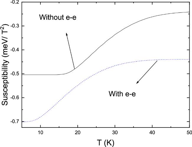
Figure 5. The susceptibility versus the temperature without SOI for $B$ = 0.5 T. |
In figure 6, the susceptibility has been presented versus temperature without and with e–e interaction taking into account Rashba SOI at zero magnetic field. As can be seen, the susceptibility displays a transition from diamagnetic to paramagnetic at a special temperature. The maximum value of the curve moves to lower temperatures in the presence of e–e interaction. Also, the width and height of the curves change with e–e interaction. By considering the SOI, there is an energy splitting as ${E}_{+}$ and ${E}_{-}.$ The occupation probability of each energy branch depends on the temperature, and e–e interaction. By considering e–e interaction, the system obtains more order at low temperatures and the susceptibility shows a maximum at low temperature.
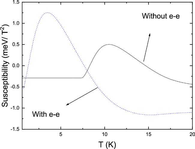
Figure 6. The susceptibility versus the temperature with SOI for $B$ = 0. |
Figure 7 demonstrates the susceptibility versus the temperature in the presence and absence of e–e interaction for $B=1\,{\rm{T}}.$ The curves were plotted in the presence and absence of the Rashba SOI. There is a paramagnetic peak in the absence of e–e interaction. The maximum value of the curve with SOI is lower than that without SOI. By increasing the temperature, the thermodynamic fluctuations enhance and the system shows a diamagnetic behavior with and without e–e interaction and Rashba SOI. We also observe that the susceptibility has negative and positive values. This means that the system shows diamagnetic and paramagnetic behaviors. The regions of diamagnetic and paramagnetic depend on the values of the temperature.
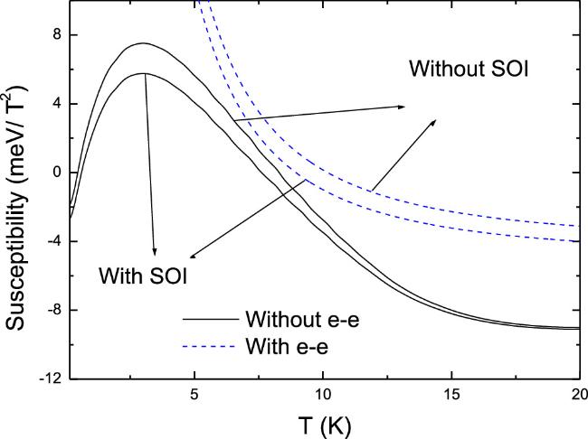
Figure 7. The susceptibility versus the temperature with SOI for $B$ = 1 T. |
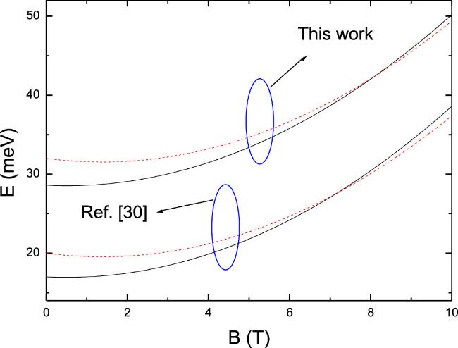
In figure 8, we plotted energies of the two low-lying states of a two-electron QD as a function of field $B$ for ${V}_{0}$ = 20 meV and ${R}_{0}$ = 10 nm. Our results have been compared with the Gaussian potential model [28]. As the magnetic field increases, the energy of the state $l$ = 0 increases but the energy of the states with non-vanishing $l$ decreases. This leads to a sequence of different ground states with $l$ = 0, −1, −2, −3, −4, … with an increase in magnetic field. An interesting phenomenon of energy level crossing happens because the coulomb energy gets smaller and smaller with increasing $\left|l\right|$ along with the average distance between the electrons. In the presence of the e–e interaction, the energy is higher because the e–e interaction is supposed to increase the total energy.
Figure 8. Energies of the two low-lying states of a two-electron QD as a function of magnetic field for ${V}_{0}$ = 20 meV and ${R}_{0}$ = 10 nm. Our results have been compared with the Gaussian potential model [28]. |
4. Conclusions
The effects of e–e interaction, Rashba SOI, and magnetic field on the susceptibility of GaAs quantum dot/ring system have been theoretically studied. According to the results, it is deduced that the magnetic field, Rashba SOI, and e–e interaction have important roles in the magnetic behavior of the system. The system can show both diamagnetic and paramagnetic behaviors with a proper selection of system parameters. The transition from paramagnetic to diamagnetic depends on temperature. It is also shown that e–e interaction causes singlet–triplet transitions in our system. The position of peak in the susceptibility has been shown to depend on the temperature and also the strength of the e–e interaction. This system can be of interest from the point of view of magnetic device applications. In future, the thermodynamic and also the magnetocaloric properties of the system in the presence of SOI can be studied.
Competing interests
The authors declare that there is no competing interests that might beperceived to influence the results and/or discussion reported in this paper.