


1. Introduction
Quantum mechanics, a fundamental theory in physics, explains the physical characteristics of atoms and subatomic particles [1]. Unlike classical mechanics, which deals with macroscopic objects and aligns with everyday intuition, quantum mechanics operates on principles that often contradict classical intuition. A key concept in quantum mechanics is wave-particle duality [2], where particles like electrons exhibit both wave-like and particle-like properties. The behavior of these particles is governed by the Schrödinger equation [3], which provides a method for calculating the probability distribution of a particle’s position and momentum [4].
Gravitational theory views gravity as the curvature of space-time rather than a force [5–7]. This perspective allows precise predictions of phenomena, such as the bending of light rays (gravitational lensing) [8–11] and gravitational waves. The current challenge in theoretical physics is the unification of quantum mechanics and general relativity theory [12–14]. While general relativity excels at describing the macroscopic world, it breaks down in extreme conditions where quantum effects are significant, such as inside black holes or at the beginning of the Universe. To address this, quantum gravity theories [15, 16], such as loop quantum gravity [17, 18] and string theory [19–21], have been developed in an attempt to create a unified framework that encompasses both of these fundamental aspects of modern physics.
Topological defects are irregularities or discontinuities that arise in ordered systems, frequently encountered in fields such as condensed matter physics and cosmology [22]. These defects emerge when the system’s order parameters fail to maintain uniformity across space. Different types of topological defects [23] include: (i) domain walls [24], which are 2D surfaces separating regions of different phases; (ii) cosmic strings [25], which are 1D lines resembling cracks in space-time; (iii) monopoles [26], which are point-like defects carrying magnetic charge; (iv) textures [27], which are 3D configurations without a distinct core. Each type of defect has distinct physical implications and is characterized by specific topological properties [28]. In condensed matter systems, such as liquid crystals and superconductors [29, 30], topological defects can significantly influence material properties and phase transitions [31]. In cosmology, these defects are believed to have formed during symmetry-breaking phase transitions in the early Universe, potentially affecting the large-scale structure of the cosmos [32]. However, the study of topological defects is constrained by the difficulty in detecting and observing them directly, especially in high-energy and large-scale contexts. Additionally, theoretical models must address the complexities of non-linear dynamics [33] and quantum field theory [34] to fully describe these defects.
In quantum systems, a harmonic oscillator serves as an analogue model of a classical harmonic oscillator [35]. Progressing further, the study of the harmonic oscillator within the context of curved space has been explored in only in a few works. These include investigations in the presence of conical singularities [36], in spaces with linear topological defects [37], the Aharonov–Bohm effect in 2D systems [38], the influence of singular potentials [39], within an elastic medium [40], and in the context of a global monopole [41, 42]. Understanding harmonic oscillators in curved space not only enriches our comprehension of classical mechanics but also provides valuable insights into the physical system in curved space. These insights have implications ranging from cosmology to quantum field theory [43].
The thermodynamic properties of quantum systems [44] exhibit different characteristics, which are distinct from those of classical systems [45]. Thermodynamic properties in quantum systems have been studied across various configurations. Notable examples include investigations in a Ga-As double ring-shaped quantum dot under external fields [46], in Rashba quantum dots with magnetic fields [47], and in asymmetric parabolic quantum dots [48, 49]. Other studies have explored these properties, such as within the framework of cosmic string space-time [50], relativistic quantum oscillators [51], and quantum oscillators with diatomic molecules [52]. Other research works in this direction are reported in [53–55].
Additional studies have focused on 1D Dirac oscillators [56], quantum fractional Dirac oscillators [57], and scalar bosons [58] in Rindler space-time. Research has also been conducted on deformed Dirac oscillators in one and two dimensions [59], the impact of minimal length effects on Dirac oscillators [60], Klein–Gordon (KG) oscillator in noncommutative space [61], and q-deformed relativistic Dirac oscillators with minimal length considerations [62]. Moreover, the properties of a 3D Dirac oscillator in noncommutative space [63] and with an Aharonov–Bohm field and magnetic monopole potential [64], anharmonic oscillators under cosmic string effects [65], and systems in disclination backgrounds with different potentials [66–73] have been thoroughly investigated.
In the current study, the main motivation is to investigate the thermodynamics of a harmonic oscillator in a conical geometry under the influence of a Wu–Yang magnetic monopole (WYMM), and an inverse square potential. We solve the wave equation using special functions and obtain the energy levels in a compact form. Subsequently, the thermodynamic behavior of the harmonic oscillator is studied at T ≠ 0 and we obtain an expression of the partition function Z. We then calculate the thermodynamic variables, such as the vibrational free energy (F), the mean free energy (U), the specific heat (${ \mathcal C }$ ), and the entropy (${ \mathcal S }$ ) of the system. Our results show that thermodynamic variables get modified by the global monopole parameter, the strength of the WYMM, and the potential for a particular ℓ-state. In contrast, the specific heat capacity and entropy only depend on the topological parameter but are independent of the WYMM and the chosen potential.
This paper is organized as follows: in section 2 , we solve the harmonic oscillator problem in a conical geometry without and with a potential. There, we study the thermodynamics of the system without a potential in section 2.1 and with a potential in section 2.2 . Finally, our conclusions are presented in section 3 .
2. Effects of conical singularity and WYMM under a potential on the harmonic oscillator system
We investigate the harmonic oscillator in a conical singularity metric and discuss the thermodynamic properties. Therefore, we begin this section by starting a conical singularity metric in the chart where (t, r, θ, φ) is given by [74] (c = 1 = ℏ = G)
$\begin{eqnarray}\begin{array}{rcl}{{\rm{d}}s}^{2} & = & -{{\rm{d}}{t}}^{2}+\displaystyle \frac{{{\rm{d}}r}^{2}}{{\alpha }^{2}}+{r}^{2}({\rm{d}}{\theta }^{2}+{\sin }^{2}\theta \,{\rm{d}}{\phi }^{2})\\ & = & -{{\rm{d}}t}^{2}+{{\rm{g}}}_{{ij}}\,{{\rm{d}}x}^{{\rm{i}}}\,{{\rm{d}}x}^{{\rm{j}}},\end{array}\end{eqnarray}$
where α is the global monopole parameter. This space-time has recently attracted considerable attention within the context of quantum systems (see, for example, [75–86]).The wave equation describing a harmonic oscillator in a quantum system under a potential V(r) is given by [86]
$\begin{eqnarray}\begin{array}{rcl} & & \left[-\displaystyle \frac{1}{2M}\,\displaystyle \frac{1}{\sqrt{{\rm{g}}}}\,{{ \mathcal D }}_{i}\left({{\rm{g}}}^{{ij}}\,\sqrt{{\rm{g}}}\,{{ \mathcal D }}_{j}\right)+\displaystyle \frac{1}{2}\,M\,{\omega }^{2}\,{\rho }^{2}+V({\boldsymbol{r}})\right]\,{\rm{\Psi }}({\boldsymbol{r}})\\ & = & E\,{\rm{\Psi }}({\boldsymbol{r}}),{{ \mathcal D }}_{i}\equiv ({\partial }_{i}-{\rm{i}}\,e\,{A}_{i}),\end{array}\end{eqnarray}$
where E is the energy, $\vec{A}$ is the three-vector potential, ${\rm{g}}=\det \ \ ({{\rm{g}}}_{{ij}})$ , and $\Psi$(r) is given by $\begin{eqnarray}{\rm{\Psi }}({\boldsymbol{r}})={\rm{R}}({r}){{\rm{Y}}}_{{{\ell }}^{{\prime} },{m}^{{\prime} }}(\theta ,\phi ),\end{eqnarray}$
with ${{\rm{Y}}}_{{{\ell }}^{{\prime} },{m}^{{\prime} }}$ given in [86, 89–91] and called the conical harmonics, and ${{\ell }}^{{\prime} },{m}^{{\prime} }$ are the effective quantum numbers.By expressing the wave equation (2 ) in the background metric, equation (1 ), using the electromagnetic potential given in [86–88] and the function in equation (3 ), we obtain the following differential equation:
$\begin{eqnarray}\begin{array}{rcl} & & {{\rm{R}}}^{{\prime\prime} }({\rm{r}})+\displaystyle \frac{2}{{r}}\,{{\rm{R}}}^{{\prime} }({\rm{r}})+\displaystyle \frac{1}{{\alpha }^{2}}\\ & & \quad \times \,\left[2\,M(E-V(r))-{{\rm{M}}}^{2}\,{\omega }^{2}\,{r}^{2}-\displaystyle \frac{{\lambda }^{{\prime} }}{{r}^{2}}\right]\,{\rm{R}}(r)=0.\end{array}\end{eqnarray}$
Below, we focus on the thermal properties of the harmonic oscillator and discuss the effects of topological defects, the strength of the WYMM, and the potential depth, if there.
2.1. Thermodynamics of the harmonic oscillator without a potential
For zero potential, V(r) = 0, the radial equation (4 ) becomes
$\begin{eqnarray}{{\rm{R}}}^{{\prime\prime} }(r)+\displaystyle \frac{2}{r}\,{{\rm{R}}}^{{\prime} }(r)+\displaystyle \frac{1}{{\alpha }^{2}}\left[2\,M\,E-{{\rm{\Omega }}}^{2}\,{r}^{2}-\displaystyle \frac{{\lambda }^{{\prime} }}{{r}^{2}}\right]\,{\rm{R}}(r)=0.\end{eqnarray}$
Performing ${\rm{R}}(r)=\tfrac{\psi (r)}{\sqrt{r}}$ , s = Ω r2 with Ω = M ω, and choosing the following function5 ) results in the confluent hypergeometric differential equation form given by [92]
$\begin{eqnarray}\psi (s)={s}^{\tfrac{\tau }{2}}\,\exp \left(-\displaystyle \frac{s}{2}\right){}_{1}{{\rm{F}}}_{1}(a,b;s)\end{eqnarray}$
in equation ( $\begin{eqnarray}s\,{\rm{F}}^{\prime\prime} (s)+(b-s){\rm{F}}^{\prime} (s)-a\,{\rm{F}}(s)=0,\end{eqnarray}$
where the function 1F1(a, b; s) is called the hypergeometric function and we defined $\begin{eqnarray}\begin{array}{rcl}a & = & \tau +\displaystyle \frac{1}{2}-\displaystyle \frac{{\rm{\Lambda }}}{4\,{\rm{\Omega }}},\quad b=\tau +1,\\ {\rm{\Lambda }} & = & \displaystyle \frac{2\,M\,E}{{\alpha }^{2}},\quad \tau =\sqrt{\displaystyle \frac{{\ell }({\ell }+1)-{\sigma }^{2}}{{\alpha }^{2}}+\displaystyle \frac{1}{4}}.\end{array}\end{eqnarray}$
Its well-known in mathematical physics that the hypergeometric function 1F1(a, b; s) becomes a finite degree polynomial provided the relation is a = − n, where n = 0, 1, 2, …. Simplification of a = − n gives us the energy level as follows [86]:9 ) and (10 ), respectively, are the energy levels and the radial function of the harmonic oscillator in topological defect geometry and a WYMM without any potential effects.
$\begin{eqnarray}{{\rm{E}}}_{n\,{\ell }\,\sigma }=2\left({\rm{n}}+\sqrt{\displaystyle \frac{{\ell }({\ell }+1)-{\sigma }^{2}}{{\alpha }^{2}}+\displaystyle \frac{1}{4}}+\displaystyle \frac{1}{2}\right)\alpha \,\omega .\end{eqnarray}$
The wave function can then be written as $\begin{eqnarray}\begin{array}{rcl}{{\rm{R}}}_{n\,{\ell }\,\sigma }(s) & = & {{\rm{\Omega }}}^{1/4}\,{s}^{\tfrac{1}{2}\left(-\tfrac{1}{2}+\sqrt{\tfrac{{\ell }({\ell }+1)-{\sigma }^{2}}{{\alpha }^{2}}+\displaystyle \frac{1}{4}}\right)}\\ & & \times \,{{\mathtt{e}}}^{-s/2}\,{}_{1}{{\rm{F}}}_{1}\left(-n,1+\sqrt{\displaystyle \frac{{\ell }({\ell }+1)-{\sigma }^{2}}{{\alpha }^{2}}+\displaystyle \frac{1}{4}};s\right).\end{array}\end{eqnarray}$
Equations (To study thermal properties, we now calculate the partition function Z(β) at T ≠ 0 by utilizing the energy expression equation (9 ). Subsequently, we will calculate other physical quantities, such as the vibrational energy, the mean free energy, the specific heat capacity, and the entropy, and analyze the outcomes. Here, β is related with the absolute temperature T as $\beta =\frac{1}{{{k}}_{{\rm{B}}}\,{T}}$ , where kB is the Boltzmann constant.
The energy expression, equation (9 ), keeping ℓ and σ constant, is given by:
$\begin{eqnarray}{E}_{n}=p\,n+q,\,p=2\,\alpha \,\omega ,\,q=(1+2\,\tau )\alpha \,\omega .\end{eqnarray}$
Partition FunctionUsing the energy expression, equation (11 ), we obtain the partition function given by:
$\begin{eqnarray}{\rm{Z}}(\alpha ,\omega ,\sigma ,{T})=\displaystyle \frac{\exp \left[-\left(\tfrac{2\,\alpha \,\omega }{{{k}}_{{\rm{B}}}\,{T}}\right)\sqrt{\tfrac{{\ell }({\ell }+1)-{\sigma }^{2}}{{\alpha }^{2}}+\tfrac{1}{4}}\right]}{2\,\sinh \left(\tfrac{\alpha \,\omega }{{{k}}_{{\rm{B}}}\,{T}}\right)}.\end{eqnarray}$
We see that Z depends on the topological parameter α, and σ, for a particular ℓ-state. Additionally, it varies with the absolute temperature T and the oscillator frequency ω. The behavior of Z as a function of kB T is illustrated in figure 1 for different values of α and ω. We see that as the values of these parameters increase, the linear increase shifts downward in the range 0 ≤ kB T ≤ 200.

Figure 1. (a)–(c) The partition function, equation ( |
Vibrational Free Energy
This is defined in terms of the partition function Z as follows:
$\begin{eqnarray}{\rm{F}}=-\displaystyle \frac{1}{\beta }\,\mathrm{lnZ}.\end{eqnarray}$
Using the partition function expression, equation (12 ), we obtain the vibrational free energy given by
$\begin{eqnarray}\begin{array}{rcl}{\rm{F}}(\alpha ,\omega ,\sigma ,{T}) & = & \alpha \,\omega \left[2\,\sqrt{\displaystyle \frac{{\ell }({\ell }+1)-{\sigma }^{2}}{{\alpha }^{2}}+\displaystyle \frac{1}{4}}\right.\\ & & \left.+\displaystyle \frac{{{k}}_{{\rm{B}}}\,{T}}{\alpha \,\omega }\,\mathrm{ln}\left(2\,\sinh \left(\displaystyle \frac{\alpha \,\omega }{{{k}}_{{\rm{B}}}\,{T}}\right)\right)\right].\end{array}\end{eqnarray}$
We see that this energy depends on the topological parameter α, and the strength of the WYMM σ, for a particular ℓ-state. Additionally, it varies with the absolute temperature T and the oscillator frequency ω. In figure 2, the behavior of the vibrational free energy, equation (15 ), is plotted as a function of kB T for different values of α and ω. It is evident that as the values of these parameters increase, the almost linear decrease shifts downward in the range 0 ≤ kB T ≤ 200.
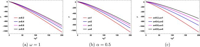
Figure 2. (a)–(c) The vibrational free energy, equation ( |
Writing $x=\tfrac{{{k}}_{{\rm{B}}}\,{T}}{\alpha \,\omega }$ , the asymptotic form of the second term within the bracket in equation (15 ) for x → 0 becomes $x\,{\rm{ln}}[2\,\sinh (1/x)]\approx 1$ . Therefore, in the limit T → 0, the asymptotic form of the vibrational free energy will be
$\begin{eqnarray}{\rm{F}}(\alpha ,\omega ,\sigma )\approx \left[2\,\sqrt{\displaystyle \frac{{\ell }({\ell }+1)-{\sigma }^{2}}{{\alpha }^{2}}+\displaystyle \frac{1}{4}}+1\right]\,\alpha \,\omega .\end{eqnarray}$
Helmholtz Free EnergyThis is defined by
$\begin{eqnarray}{\rm{U}}=-\displaystyle \frac{\partial }{\partial \beta }(\mathrm{ln}\,{\rm{Z}}).\end{eqnarray}$
Using expression (13 ), we obtain this energy given by
$\begin{eqnarray}\begin{array}{rcl}{\rm{U}}(\alpha ,\omega ,\sigma ,{T}) & = & \alpha \,\omega \left[2\,\sqrt{\displaystyle \frac{{\ell }({\ell }+1)-{\sigma }^{2}}{{\alpha }^{2}}+\displaystyle \frac{1}{4}}\right.\\ & & \left.+\,\coth \left(\displaystyle \frac{\alpha \,\omega }{{{k}}_{{\rm{B}}}\,{T}}\right)\right].\end{array}\end{eqnarray}$
We see that this Helmholtz free energy depends on the topological parameter α, and the strength of the WYMM σ, for a particular ℓ-state. Moreover, It changes with the absolute temperature T and the oscillator frequency ω. The behavior of this energy, equation (18 ), as a function of $\tfrac{1}{{{k}}_{{\rm{B}}}\,{T}}$ is plotted in figure 3 for different values of α and ω. It is evident that as the values of these parameters increase, the linear increase shifts downward in kB T > 0 (figure 3(a)–(b)). While in figure 3(c), it shows decreases in the nature of the curve in the range kB T > 0.

Figure 3. (a)–(c) The Helmholtz free energy, equation ( |
In the limit T → 0, the asymptotic form of $\coth \left(\tfrac{\alpha \,\omega }{{{k}}_{{\rm{B}}}\,{T}}\right)$ is given by
$\begin{eqnarray}\coth \left(\displaystyle \frac{\alpha \,\omega }{{{k}}_{{\rm{B}}}\,{T}}\right)\approx 1+2\,{{\mathtt{e}}}^{-\tfrac{2\,\alpha \,\omega }{{{k}}_{{\rm{B}}}\,{T}}}.\end{eqnarray}$
Therefore, the asymptotic form of the Helmholtz energy in the limit T → 0 will be $\begin{eqnarray}\begin{array}{l}{\rm{U}}(\alpha ,\omega ,\sigma ,{T})\\ \quad \approx \,\left[2\,\sqrt{\displaystyle \frac{{\ell }({\ell }+1)-{\sigma }^{2}}{{\alpha }^{2}}+\displaystyle \frac{1}{4}}+1+2\,{{\mathtt{e}}}^{-\tfrac{2\,\alpha \,\omega }{{{k}}_{{\rm{B}}}\,{T}}}\right]\,\alpha \,\omega .\end{array}\end{eqnarray}$
Specific Heat CapacityThis is defined by
$\begin{eqnarray}\displaystyle \frac{{ \mathcal C }}{{{k}}_{{\rm{B}}}}={\beta }^{2}\,\displaystyle \frac{{\partial }^{2}}{\partial {\beta }^{2}}(\mathrm{lnZ}).\end{eqnarray}$
Using expression (13 ), we obtain the specific heat capacity given by
$\begin{eqnarray}\displaystyle \frac{{ \mathcal C }(\alpha ,\omega ,{T})}{{{k}}_{{\rm{B}}}}=\displaystyle \frac{{\alpha }^{2}\,{\omega }^{2}}{{{k}}_{{\rm{B}}}^{2}\,{{T}}^{2}}\,\displaystyle \frac{1}{{\sinh }^{2}\left(\tfrac{\alpha \,\omega }{{{k}}_{{\rm{B}}}\,{T}}\right)}.\end{eqnarray}$
One can see that the heat capacity depends only on the topological parameter α for a particular ℓ-state and changes with the absolute temperature T and the oscillator frequency ω. In figure 4, the behavior of the specific heat capacity, equation (22 ), is plotted as a function of $\tfrac{1}{{{k}}_{{\rm{B}}}\,{T}}$ for different values of α and ω. It is evident that as the values of these parameters increase, the nature of the decreasing curves shifts downward in the range kB T > 0.
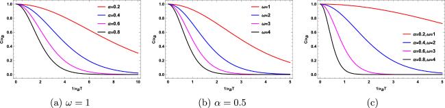
Figure 4. (a)–(c) The specific heat capacity of equation ( |
Writing $x=\tfrac{{{k}}_{{\rm{B}}}\,{T}}{\alpha \,\omega }$ , equation (22 ) can be written as
$\begin{eqnarray}\displaystyle \frac{{ \mathcal C }(\alpha ,\omega ,{T})}{{{k}}_{{\rm{B}}}}=\displaystyle \frac{1}{{x}^{2}\,{\sinh }^{2}\left(\tfrac{1}{x}\right)}.\end{eqnarray}$
In the limit x → 0, the asymptotic expansion of the above equation is given by $\begin{eqnarray}\displaystyle \frac{{ \mathcal C }(\alpha ,\omega ,{T})}{{{k}}_{{\rm{B}}}}\approx {\left(\displaystyle \frac{2\,\alpha \,\omega }{{{k}}_{{\rm{B}}}\,{T}}\right)}^{2}\,{{\mathtt{e}}}^{-\tfrac{2\,\alpha \,\omega }{{{k}}_{{\rm{B}}}\,{T}}}.\end{eqnarray}$
This shows that the specific heat capacity decays very rapidly due to the exponential factor.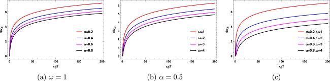
Figure 5. (a)–(c) The entropy of equation ( |
We have generated figure 6 showing this asymptotic form of the specific heat capacity as a function of κB T for different values of the topological parameter 0 < α ≤ 1, keeping the frequency ω = 0.1 > 0 fixed. It is clear from this figure that this vanishes as T approaches zero.

Figure 6. The behavior of the asymptotic specific heat capacity as a function of T. Here, ω = 0.1. |
Entropy
This is defined by
$\begin{eqnarray}\displaystyle \frac{{ \mathcal S }}{{{k}}_{{\rm{B}}}}=\mathrm{lnZ}-\beta \,\displaystyle \frac{\partial }{\partial \beta }(\mathrm{lnZ}).\end{eqnarray}$
Using expression (13 ), we obtain the entropy of the system given by
$\begin{eqnarray}\displaystyle \frac{{ \mathcal S }(\alpha ,\omega ,{T})}{{{k}}_{{\rm{B}}}}=\displaystyle \frac{\alpha \,\omega }{{{k}}_{{\rm{B}}}\,{T}}\,\coth \left(\displaystyle \frac{\alpha \,\omega }{{{k}}_{{\rm{B}}}\,{T}}\right)-\mathrm{ln}\left[2\,\sinh \left(\displaystyle \frac{\alpha \,\omega }{{{k}}_{{\rm{B}}}\,{T}}\right)\right].\end{eqnarray}$
We see that the entropy of the system depends only on the topological parameter α for a particular ℓ-state and changes with the absolute temperature T and the oscillator frequency ω . In figure 5, the entropy behavior, equation (26 ), is plotted as a function of kB T and observed to be parabolic in nature. It is evident that as the values of these parameters increase, the parabolic nature shifts downward in the range 0 ≤ kB T ≤ 200.
Writing $x=\tfrac{{k}_{{\rm{B}}}\,T}{\alpha \,\omega }$ , equation (26 ) can be written as
$\begin{eqnarray}\displaystyle \frac{{ \mathcal S }(\alpha ,\omega ,{T})}{{{k}}_{{\rm{B}}}}=\displaystyle \frac{\coth \left(\tfrac{1}{{\rm{x}}}\right)}{{\rm{x}}}-\mathrm{ln}\left[2\,\sinh \left(\displaystyle \frac{1}{{\rm{x}}}\right)\right].\end{eqnarray}$
In the limit x → 0, the asymptotic expansion of entropy is given by $\begin{eqnarray}\displaystyle \frac{{ \mathcal S }(\alpha ,\omega ,{T})}{{{k}}_{{\rm{B}}}}\approx \displaystyle \frac{2\,\alpha \,\omega }{{{k}}_{{\rm{B}}}\,{T}}\,{{\mathtt{e}}}^{-\tfrac{2\,\alpha \,\omega }{{{k}}_{{\rm{B}}}\,{T}}}.\end{eqnarray}$
This shows that entropy of the quantum system decays exponentially as T approaches zero.We have generated figure 7 showing this asymptotic form of entropy as a function of κB T for different values of the topological parameter 0 < α ≤ 1, keeping the frequency ω = 0.1 > 0 fixed. It is clear from this figure that entropy vanishes as T approaches zero.

Figure 7. The behavior of the asymptotic entropy form as a function of T. Here, ω = 0.1 |
In summary, we have examined the thermodynamics of a harmonic oscillator without a potential in a conical geometry and in a WYMM. Figures (1)–(7) illustrate how thermodynamic variables, such as the partition function, the vibrational free energy, the Helmholtz free energy, the specific heat capacity, and entropy, are influenced by various parameters. These figures demonstrate the dependence of thermodynamic variables on the topological parameter α, and the strength of the WYMM σ. Notably, we have observed that the specific heat capacity and entropy of the system are independent of the strength of the WYMM.
2.2. Thermodynamics of the harmonic oscillator with a potential
Here, we consider an inverse square potential ${\rm{V}}(r)=\tfrac{\eta }{{r}^{2}}$ , where η > 0 is a constant. Using this potential, we find the radial equation as follows:
$\begin{eqnarray}\begin{array}{rcl} & & {{\rm{R}}}^{{\prime\prime} }(r)+\displaystyle \frac{2}{r}\,{{\rm{R}}}^{{\prime} }(r)+\left[\displaystyle \frac{2\,M\,E}{{\alpha }^{2}}-{{\rm{\Omega }}}^{2}\,{r}^{2}-\displaystyle \frac{{\lambda }^{{\prime} }+2\,M\,\eta }{{\alpha }^{2}\,{r}^{2}}\right]\\ & & \quad \times \,{\rm{R}}(r)=0.\end{array}\end{eqnarray}$
Performing ${\rm{R}}(r)=\tfrac{\psi (r)}{\sqrt{r}}$ , s = Ω r2 with Ω = M ω, and inserting the following function29 ) results in the confluent hypergeometric differential equation form [92] given by
$\begin{eqnarray}\psi (s)={s}^{\iota /2}\,\exp (-s/2){}_{1}{{\rm{F}}}_{1}(c,d;s)\end{eqnarray}$
into equation ( $\begin{eqnarray}s\,{\rm{F}}^{\prime\prime} (s)+({\rm{d}}-s){\rm{F}}^{\prime} (s)-{\rm{c}}\,{\rm{F}}(s)=0,\end{eqnarray}$
with 1F1(c, d, s) called the confluent hypergeometric function, and we define $\begin{eqnarray}\begin{array}{l}c=\iota +\displaystyle \frac{1}{2}-\displaystyle \frac{{\rm{\Lambda }}}{4\,{\rm{\Omega }}},\quad d=1+\iota ,\\ \quad \iota =\sqrt{\displaystyle \frac{{\ell }({\ell }+1)-{\sigma }^{2}+2\,{\rm{M}}\,\eta }{{\alpha }^{2}}+\displaystyle \frac{1}{4}}.\end{array}\end{eqnarray}$
Following the previous procedure and after some calculation, we find the energy levels given by
$\begin{eqnarray}{E}_{n\,{\ell }\sigma }=2\left(n+\sqrt{\displaystyle \frac{{\ell }({\ell }+1)-{\sigma }^{2}+2\,{\rm{M}}\,\eta }{{\alpha }^{2}}+\displaystyle \frac{1}{4}}+\displaystyle \frac{1}{2}\right)\alpha \,\omega .\end{eqnarray}$
The radial function is given by $\begin{eqnarray}\displaystyle \begin{array}{rcl}{{\rm{R}}}_{n\,{\ell }}\sigma (s) & = & {{\rm{\Omega }}}^{1/4}\,{s}^{\displaystyle \frac{1}{2}\left(-\displaystyle \frac{1}{2}+\sqrt{\displaystyle \frac{{\ell }({\ell }+1)-{\sigma }^{2}+2\,{\rm{M}}\,\eta }{{\alpha }^{2}}+\displaystyle \frac{1}{4}}\right)}\\ & & \times \,{{\mathtt{e}}}^{-s/2}\,{}_{1}{{\rm{F}}}_{1}\left(-n,1+\sqrt{\displaystyle \frac{{\ell }({\ell }+1)-{\sigma }^{2}+2\,{\rm{M}}\,\eta }{{\alpha }^{2}}+\displaystyle \frac{1}{4}};s\right).\end{array}\end{eqnarray}$
Equation (33 ) is the energy level and equation (34 ) is the radial function of the harmonic oscillator in the conical metric and in a WYMM under the influence of an inverse square potential. We see that the energy level is influenced by various factors, such as the strength of the WYMM (σ), the topological parameter (α), and the potential parameter (η).
Here, we will also study thermal properties at T ≠ 0 and analyze the results. The energy expression, equation (33 ), keeping ℓ and σ constant, can be written as
$\begin{eqnarray}{{\rm{E}}}_{n}=p\,n+\tilde{q},\,p=2\,\alpha \,\omega ,\,\tilde{q}=(1+2\,\iota )\alpha \,\omega .\end{eqnarray}$
Using the above energy expression, equation (35 ), we obtain the partition function given by
$\begin{eqnarray}{\rm{Z}}(\alpha ,\omega ,\sigma ,\eta ,{T})=\displaystyle \frac{\exp \left[-\tfrac{2\,\alpha \,\omega }{{{k}}_{{\rm{B}}}\,{T}}\,\sqrt{\tfrac{{\ell }({\ell }+1)-{\sigma }^{2}+2\,{\rm{M}}\,\eta }{{\alpha }^{2}}+\displaystyle \frac{1}{4}}\right]}{2\,\sinh \left(\displaystyle \frac{\alpha \,\omega }{{{k}}_{{\rm{B}}}\,{T}}\right)}.\end{eqnarray}$
The partition function Z depends on several parameters: the topological parameter α, the strength of the WYMM σ, and the potential strength η for a particular ℓ-state. Additionally, It varies with the absolute temperature T and the oscillator frequency ω. The behavior of this function, equation (36 ), for ℓ = 0- and ℓ = 1-states is illustrated in figures (8) and (9). As shown, the partition function exhibits a linear relationship with kB T > 0 for specific values of (α, ω). This linear trend shifts downward with increasing values of α, ω η, while keeping σ fixed.

Figure 8. (a)–(f) The partition function, equation ( |
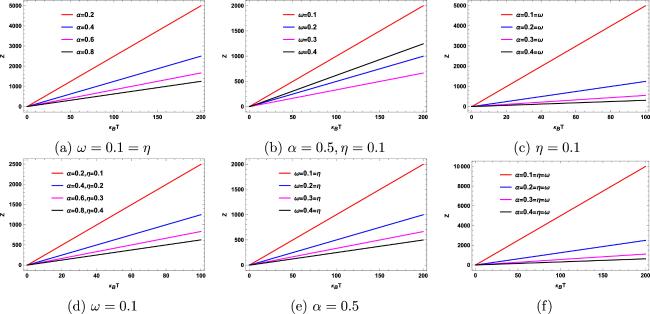
Figure 9. (a)–(f) The partition function, equation ( |
Vibrational Free Energy
The vibrational free energy using equation (36 ) is given by
$\begin{eqnarray}\begin{array}{rcl}{\rm{F}}(\alpha ,\omega ,\sigma ,\eta ,{T}) & = & 2\,\alpha \,\omega \,\sqrt{\displaystyle \frac{{\ell }({\ell }+1)-{\sigma }^{2}+2\,{\rm{M}}\,\eta }{{\alpha }^{2}}+\displaystyle \frac{1}{4}}\\ & & +\,{{k}}_{{\rm{B}}}\,{T}\,\mathrm{ln}\left[2\,\sinh \left(\displaystyle \frac{\alpha \,\omega }{{{k}}_{{\rm{B}}}\,{T}}\right)\right].\end{array}\end{eqnarray}$
This energy depends on several factors, such as the topological parameter α, the strength of the WYMM σ, and the potential strength η for a particular ℓ-state. Moreover, it changes with the absolute temperature T and the oscillator frequency ω. The behavior of this energy, equation (37 ) for ℓ = 0 and ℓ = 1-states is depicted in figures (10) and (11). It is clear from these figures that this energy decreases with increasing kB T for particular values of α, ω, and η. These decreasing trends shift upward with increasing values of the aforementioned parameters in the range 0 < kB T ≤ 5.

Figure 10. (a)–(f) The vibrational free energy, equation ( |

Figure 11. (a)–(f) The vibrational free energy, equation ( |
In the limit T → 0, the asymptotic form of the vibrational free energy is given by
$\begin{eqnarray}\begin{array}{l}{\rm{F}}(\alpha ,\omega ,\sigma ,\eta )\approx \left[2\,\sqrt{\displaystyle \frac{{\ell }({\ell }+1)-{\sigma }^{2}+2\,{\rm{M}}\,\eta }{{\alpha }^{2}}+\displaystyle \frac{1}{4}}+1\right]\,\alpha \,\omega .\end{array}\end{eqnarray}$
Helmholtz Free EnergyThe mean energy using equation (36 ) is given by
$\begin{eqnarray}\begin{array}{rcl} & & {\rm{U}}(\alpha ,\omega ,\sigma ,\eta ,{T})\\ & & \quad =\,\alpha \,\omega \left[2\,\sqrt{\displaystyle \frac{{\ell }({\ell }+1)-{\sigma }^{2}+2\,{\rm{M}}\,\eta }{{\alpha }^{2}}+\displaystyle \frac{1}{4}}+\coth \left(\displaystyle \frac{\alpha \,\omega }{{{k}}_{{\rm{B}}}\,{T}}\right)\right].\end{array}\end{eqnarray}$
The Helmholtz energy depends on the topological parameter α, the strength of the WYMM σ, and the potential strength η for a particular ℓ-state. Additionally, it varies with the absolute temperature T and the oscillator frequency ω. The behavior of the Helmholtz energy, equation (39 ), for ℓ = 0- and ℓ = 1-states is illustrated in figures (12) and (13). As shown, this energy is almost linear with increasing $\tfrac{1}{{{k}}_{{\rm{B}}}\,{T}}$ for particular values of α, ω, and η. This linear trend shifts upward with increasing values of these parameters (α, ω, η) when $\tfrac{1}{{{k}}_{{\rm{B}}}\,{T}}\gt 0$ .

Figure 12. (a)–(f) The Helmholtz free energy, equation ( |

Figure 13. (a)–(f) The Helmholtz free energy, equation ( |
The asymptotic form of Helmholtz energy in the limit T → 0 becomes
$\begin{eqnarray}\begin{array}{rcl} & & {\rm{U}}(\alpha ,\omega ,\sigma ,\eta ,{T})\\ & \approx & \alpha \,\omega \left[2\,\sqrt{\frac{{\ell }({\ell }+1)-{\sigma }^{2}+2\,{\rm{M}}\,\eta }{{\alpha }^{2}}+\frac{1}{4}}+1+2\,{{\mathtt{e}}}^{-\frac{2\,\alpha \,\omega }{{{k}}_{{\rm{B}}}\,{T}}}\right].\end{array}\end{eqnarray}$
Specific Heat CapacityUsing expression (36 ), we find the specific heat capacity given by22 ).
$\begin{eqnarray}\displaystyle \frac{{ \mathcal C }(\alpha ,\omega ,{T})}{{{k}}_{{\rm{B}}}}={\left(\displaystyle \frac{\alpha \,\omega }{{{k}}_{{\rm{B}}}\,{T}}\right)}^{2}\,\displaystyle \frac{1}{{\sinh }^{2}\left(\tfrac{\alpha \,\omega }{{{k}}_{{\rm{B}}}\,{T}}\right)},\end{eqnarray}$
which is similar to the previous result, equation (The specific heat capacity depends only on the topological parameter α for a particular ℓ-state. Additionally, it changes with the absolute temperature T and the oscillator frequency ω. Interestingly, it is independent of the potential and the WYMM interaction. Therefore, its behavior closely resembles that depicted in figure 4.
Entropy
Using expression (13 ), we obtain the entropy of the system given by26 ).
$\begin{eqnarray}\displaystyle \frac{\left.{ \mathcal S }(\alpha ,\omega ,T\right)}{{k}_{{\rm{B}}}}=\displaystyle \frac{\alpha \,\omega }{{k}_{{\rm{B}}}\,T}\,\coth \left(\displaystyle \frac{\alpha \,\omega }{{k}_{{\rm{B}}}\,T}\right)-{\rm{ln}}\left[2\,\sinh \left(\displaystyle \frac{\alpha \,\omega }{{k}_{{\rm{B}}}\,T}\right)\right],\end{eqnarray}$
which is similar to the previous result, equation (This entropy depends only on the topological parameter α for a particular ℓ-state. Moreover, it changes with the absolute temperature T and the oscillator frequency ω. Interestingly, we see that it is independent of the potential and the WYMM interaction. Therefore, its behavior closely resembles that depicted in figure 5.
In summary, we have examined the thermal properties of a harmonic oscillator under potential effects in a conical metric and in a WYMM. Figures (8)–(13) illustrate how thermodynamic variables, such as the partition function, vibrational free energy, Helmholtz free energy, specific heat capacity, and entropy are influenced by. These figures demonstrate the dependence of thermodynamic variables on the topological parameter α, the strength of the WYMM σ, and the potential strength η. Notably, we have observed that the specific heat capacity and entropy are independent of the potential and the strength of the WYMM.
3. Conclusions
In this current work, we examined the thermodynamic properties of a harmonic oscillator in a conical metric and a WYMM under a potential. We solved the wave equation and obtained a compact form of the energy levels and the radial wave function using special functions, both without and with a potential.
In section 2.1 , we studied the thermodynamics of the system without a potential and obtained thermodynamic variables, including the partition function, the vibrational free energy, the Helmholtz free energy, the specific heat capacity, and entropy. It has been demonstrated that these variables, except for the specific heat capacity and entropy, depend on the topological parameter α and the strength of the WYMM σ. We depicted several figures illustrating the behavior of these variables as a function of $\tfrac{1}{\beta }={{k}}_{{\rm{B}}}\,{T}$ for different values of the aforementioned parameters, including the oscillator frequency.
In section 2.2 , we introduced an inverse square potential and studied the thermodynamics of the system. Similar to the previous section, we analyzed the partition function, the vibrational free energy, the Helmholtz free energy, the specific heat capacity, and entropy. We have demonstrated that these physical quantities vary with the potential in addition to those parameters mentioned earlier in the previous paragraph. Again, it was observed that the specific heat capacity and entropy are independent of the strength of the WYMM and the potential. We have provided graphs illustrating the behavior of these thermodynamic variables as a function of $\tfrac{1}{\beta }={{k}}_{{\rm{B}}}\,{T}$ for different values of various parameters.
The investigation into the thermodynamics of a harmonic oscillator in conical geometry, featuring a WYMM and an inverse square potential, provided intriguing insights into the interplay between quantum mechanics and a classical thermodynamic system. Through rigorous analysis, we have elucidated the impact of the global monopole parameter characterized by α. Moreover, the presence of the WYMM introduces non-trivial magnetic interactions, altering the dynamics of the harmonic oscillator and, thereby, changing the thermodynamic behavior. Additionally, the inclusion of an inverse square potential modified the solution of the wave equation, leading to changes in the thermodynamic properties.
We have depicted several figures (figures (1)–(13)) illustrating the partition function, vibrational energy, Helmholtz energy, specific heat capacity, and entropy as functions of kB T and, in some cases, $\tfrac{1}{{{k}}_{{\rm{B}}}\,{T}}$ for specific values of (α, ω, η) while keeping the WYMM strength σ and ℓ constant. Additionally, we have varied the values of these parameters to demonstrate how they influence the behavior of these thermodynamic functions.
These findings not only deepen our theoretical understanding of quantum systems in the presence of topological defects but also pave the way for potential applications in diverse fields, ranging from condensed matter physics to quantum information processing. Notably, we have observed that the specific heat capacity and entropy are independent of both the potential and the strength of the WYMM.
In our upcoming work, we will investigate the quantum equipartition theorem as it applies to the current system, following the approach outlined in [97]. We will also analyze the results obtained from this study and discuss the effects of conical singularity and the WYMM.
Acknowledgments
We sincerely acknowledge the anonymous referees for their valuable remarks and suggestions. FA acknowledges the Inter University Centre for Astronomy and Astrophysics (IUCAA), Pune, India for granting a visiting associateship.