Welcome to visit Communications in Theoretical Physics,
Gravitation Theory, Astrophysics and Cosmology

Cosmography of non-interacting ghost and generalized ghost dark energy models in f(Q) gravity

  • M Sharif ,
  • Madiha Ajmal
Expand
  • Department of Mathematics and Statistics, The University of Lahore, 1-KM Defence Road, Lahore 54000, Pakistan

Received date: 2024-08-23

  Revised date: 2024-10-23

  Accepted date: 2024-10-31

  Online published: 2025-01-07

Copyright

© 2025 Institute of Theoretical Physics CAS, Chinese Physical Society and IOP Publishing. All rights, including for text and data mining, AI training, and similar technologies, are reserved.
This article is available under the terms of the IOP-Standard License.

Abstract

This paper aims to develop non-interacting ghost dark energy and generalized ghost dark energy models within the framework of f(Q) theory using the correspondence scheme. We use pressureless matter and a power-law scale factor. The cosmic implications of the resulting models are studied through the equation of state parameter and the phase planes. We also check the stability of the reconstructed models through the squared speed of sound parameter. The equation of state parameter exhibits a phantom era, the $({\omega }_{D}-{\omega }_{D}^{{\prime} })$ -plane indicates a freezing region, while the (rs)-plane corresponds to the Chaplygin gas model for both models. It is also found that only the generalized ghost dark energy model remains stable throughout cosmic evolution. We conclude that our findings align well with current observational data.

Cite this article

M Sharif , Madiha Ajmal . Cosmography of non-interacting ghost and generalized ghost dark energy models in f(Q) gravity[J]. Communications in Theoretical Physics, 2025 , 77(4) : 045402 . DOI: 10.1088/1572-9494/ad8db8

1. Introduction

Cosmology represents one of the most complex domains of astronomy [1, 2], focusing on the study of the cosmic structure as well as its origin and evolutionary trajectory. It encompasses an exploration of fundamental questions about the Universe such as its composition, behavior and ultimate fate. The general theory of relativity (GR) established the basis for contemporary cosmology. One of the most notable accomplishments in this field is the rapid expansion of the cosmos which has been confirmed by various cosmological observations such as Supernovae type-Ia [3], large-scale structure [4]–[6] and cosmic microwave background radiation [7]. The accelerated expansion of cosmos has been attributed to a mysterious form of energy known as dark energy (DE). This enigmatic form of energy is evenly spread throughout the cosmos with an ambiguous nature. The Λ cold dark matter (ΛCDM) model depends on the cosmological constant and serves as the fundamental framework for understanding DE. Despite its consistency with observational data, the ΛCDM model faces several challenges including issues like fine-tuning and the cosmic coincidence problems [8]–[10]. To comprehend the nature of DE, researchers employed two different methods. Firstly, by examining DE models and secondly, through the use of modified gravity theories.
Every DE model contains many concealed and distinct characteristics, leading to a challenging scenario to researchers. Most DE models typically involve an additional degree of freedom to account for the current state of the cosmos [11, 12]. This additional factor may lead to inconsistency in the outcomes. For a satisfactory DE model, it is crucial to solve this issue without depending on any new degree of freedom or an extra parameter. A novel form of DE called Veneziano ghost DE (GDE) has been suggested to achieve this purpose [13, 14]. The energy density of the GDE model is represented as
$\begin{eqnarray}{\rho }_{D}=\alpha H,\end{eqnarray}$
where α denotes an arbitrary constant with dimensions of [energy]3. The GDE arises from the need to account for the observed accelerated expansion of the Universe without resorting to the introduction of exotic form of matter or energy. By considering such unconventional energy configurations, GDE models aim to explain cosmic acceleration while remaining consistent with theoretical principles and observational constraints.
The GDE presents a fascinating concept in cosmology. In simple terms, the ghost field contribution to vacuum energy varies depending on the type of spacetime. This contribution scales proportionally with ${\Lambda }_{\mathrm{QCD}}^{3}H,$ where ΛQCD represents the quantum chromodynamics (QCD) [15]–[19] mass scale. In the GDE model, the vacuum energy associated with the ghost field behaves similar to a dynamic cosmological constant. Extensive research has been delved into various aspects of GDE. This model deals with certain issues effectively but it faces stability challenges [20, 21]. It is found that the Veneziano QCD ghost field's contribution to vacuum energy is not exactly of order H but rather involves a subleading term H2, known as the generalized GDE (GGDE) model. The density of this GGDE is described as
$\begin{eqnarray}{\rho }_{D}=\alpha H+\beta {H}^{2},\end{eqnarray}$
where β denotes another arbitrary constant with dimensions of [energy]2. This model is an exciting area in cosmology that aims to uncover the mysterious nature of DE. This theoretical framework extends beyond traditional models, incorporating ghost fields to address shortcomings and offers fresh insights into the rapid expansion of the cosmos. This model studies ghost-like fields in the Universe to better understand how the Universe evolves and its overall structure.
The current rapid expansion of the cosmos can be explored through various models of DE. Researchers often use reconstruction techniques in modified gravity theories to create DE models that explain the Universe acceleration. This process compares the energy densities of the DE model and modified gravity theory. The correspondence between these energy densities has been widely explored in various DE models in the literature. Using the correspondence scheme, we examine how these models work together to enhance our understanding of cosmic acceleration. This method helps to connect theoretical predictions with observational data, offering a deep understanding of how DE and modified gravity contribute. Saaidi et al [22] used a correspondence scheme to reconstruct the GDE f(R) model (R represents the Ricci scalar) to examine its stability and evolution through the analysis of cosmological parameters. Sheykhi and Movahed [23] examined the implications of the same model in GR by observing the expansion of the cosmos through limitations on the model parameter. Sadeghi et al [24] discussed the interaction of this model by modifying both the gravitational constant and the cosmological constant. They conducted numerical computations to study the behavior of the Universe through the equation of state (EoS) and deceleration parameters. Fayaz et al [25] explored this concept by studying f(R) gravity to analyze the Universe evolution.
Chattopadhyay [26] discussed two realistic f(T) models (T is the torsion scalar) and examined their stability using the squared speed of sound and EoS parameter. Pasqua et al [27] explored DE within the framework of $f(R,{\mathbb{T}})$ gravity (${\mathbb{T}}$ is the trace of the energy–momentum tensor (EMT)), incorporating a higher order of the Hubble parameter. Fayaz et al [28] studied this concept within $f(R,{\mathbb{T}})$ gravity and determined that their findings support the present state of the cosmos. Sharif and Saba [29, 30] proposed a reconstruction of GDE and GGDE within the framework of modified Gauss–Bonnet gravity. Liu [31] studied the dynamics of the scalar field to characterize intricate quintessence cosmology through the ghost model of interacting DE. Zarandi and Ebrahimi [32] studied the cosmic age problem in holographic DE and GGDE models. Sharif and Ibrar [33] discussed the reconstructed GDE $f(Q,{\mathbb{T}})$ gravity model (Q is the non-metricity) for the non-interacting case.
The Levi-Civita (LC) connection, which is torsion-free but compatible with metric, forms the foundation of GR. This was replaced in flat spacetime with a metric-compatible affine connection that includes torsion. In this alternative framework, torsion was permitted to fully characterize gravity. This particular concept was first suggested by Einstein referred to as the metric teleparallel gravity [34]–[36]. The symmetric teleparallel theory, a recent addition to this family of theories, utilizes an affine connection with zero curvature and torsion. This theory explores gravity by emphasizing the non-metricity of spacetime [37]. In metric teleparallelism, the torsion scalar is derived from the torsion tensor, whereas in the symmetric teleparallel framework, the non-metricity scalar Q is used for this purpose. By using the Lagrangian $L=\sqrt{-g}T$ [38] for the metric teleparallel theory and $L=\sqrt{-g}Q$ [39] for the symmetric teleparallel theory, we can derive their field equations. Both theories are equivalent to GR except for a boundary term. Consequently, both metric and symmetric teleparallel theories address the same DE issues as GR. To tackle this problem, new concepts related to gravity, like f(T) and f(Q) have been put forward in their specific frameworks. It is important to highlight that the teleparallel theory differs from GR as the affine connection is not linked to the metric tensor. Consequently, teleparallel theories are classified within the broader category of metric-affine theories, where both the metric and the connection serve as dynamic variables. Notably, f(T) and f(Q) theories offer an advantage over f(R) as they feature second-order field equations rather than fourth-order ones. This distinction could offer a different explanation for the observed acceleration of cosmic expansion [40]–[45].
Researchers are highly interested in investigating non-Riemannian geometry, particularly, the f(Q) theory of gravity. Frusciante [46] proposed a particular model within this gravity framework that showed foundational similarities to the ΛCDM model. Ayuso et al [47] performed the comparison between the new cosmologies and the ΛCDM setup and carried out the statistical tests based on background observational data. Solanki et al [48] investigated the impact of bulk viscosity in f(Q) gravity to explore cosmic accelerated expansion. Albuquerque and Frusciante [49] investigated the evolution of linear perturbations under the same theory. Sokoliuk et al [50] described the evolution of the cosmos through Pantheon data sets in this theory. Esposito et al [51] focused on employing the reconstruction technique to investigate the precise isotropic and anisotropic cosmological solutions in the same background. In a recent paper [52], we have investigated the cosmography of GGDE within the interacting scenario under the same gravity framework. Gadbail and Sahoo [53] studied three different models of this to determine which one more accurately expresses theoretical evolution of the ΛCDM model. Sharif et al [54] investigated the concept of a cosmological bounce within the framework of non-Riemannian geometry.
This paper examines the reconstruction of GDE and GGDE f(Q) models in the non-interacting scenario using a correspondence scheme. We explore the evolution of the cosmos by analyzing the EoS, phase planes and the squared speed of sound (${\nu }_{s}^{2}$ ). The article is structured as follows. Section 2 outlines the details of this modified theory of gravity. We also discuss non-interacting DE and DM in the FRW universe background. In sections 3 and 4, we explore a correspondence technique to reconstruct both models in f(Q) gravity. Finally, section 5 presents a summary of our findings.

2. Overview of f(Q) theory

A connection which is both torsion-free as well as compatible with the metric tensor is the LC connection [55]. However, it is possible to define two rank-3 tensors, torsion tensor $({T}_{\psi \gamma }^{\lambda })$ and non-metricity tensor (Qγ$\Psi$σ), associated with the asymmetric tensor and covariant derivative of the metric tensor, respectively, as
$\begin{eqnarray}{T}_{\psi \gamma }^{\lambda }=2{\hat{{\rm{\Gamma }}}}_{[\psi \gamma ]}^{\lambda },\,\,{Q}_{\gamma \psi \sigma }={{\rm{\nabla }}}_{\sigma }{g}_{\gamma \psi }\ne 0.\end{eqnarray}$
In this type of spacetime, the asymmetric tensor [56] can be represented as
$\begin{eqnarray}{\hat{{\rm{\Gamma }}}}_{\psi \gamma }^{\lambda }={{\rm{\Gamma }}}_{\psi \gamma }^{\lambda }+{{\mathbb{C}}}_{\psi \gamma }^{\lambda }+{{\mathbb{L}}}_{\psi \gamma }^{\lambda },\end{eqnarray}$
where, the LC connection is given as follows
$\begin{eqnarray}{{\rm{\Gamma }}}_{\psi \gamma }^{\lambda }=\frac{1}{2}{g}^{\lambda \sigma }({g}_{\sigma \psi ,\gamma }+{g}_{\sigma \gamma ,\psi }-{g}_{\psi \gamma ,\sigma }),\end{eqnarray}$
the contortion tensor is expressed as
$\begin{eqnarray}{{\mathbb{C}}}_{\psi \gamma }^{\lambda }={\hat{{\rm{\Gamma }}}}_{[\psi \gamma ]}^{\lambda }+{g}^{\lambda \sigma }{g}_{\psi \kappa }{\hat{{\rm{\Gamma }}}}_{[\gamma \sigma ]}^{\kappa }+{g}^{\lambda \sigma }{g}_{\gamma \kappa }{\hat{{\rm{\Gamma }}}}_{[\psi \sigma ]}^{\kappa }\end{eqnarray}$
and the disformation tensor is given by
$\begin{eqnarray}{{\mathbb{L}}}_{\psi \gamma }^{\lambda }=\frac{1}{2}{g}^{\lambda \sigma }({Q}_{\gamma \psi \sigma }+{Q}_{\psi \gamma \sigma }-{Q}_{\lambda \psi \gamma }).\end{eqnarray}$
Within the framework of symmetric connection, the LC connection can be expressed in terms of the disformation tensor as follows
$\begin{eqnarray}{{\rm{\Gamma }}}_{\gamma \psi }^{\lambda }=-{{\mathbb{L}}}_{\gamma \psi }^{\lambda }.\end{eqnarray}$
In GR, it is widely acknowledged that the gravitational action can be rewritten into a non-covariant form as
$\begin{eqnarray}S=\frac{1}{2k}\int {g}^{\gamma \psi }({{\rm{\Gamma }}}_{\sigma \gamma }^{\mu }{{\rm{\Gamma }}}_{\psi \mu }^{\sigma }-{{\rm{\Gamma }}}_{\sigma \mu }^{\mu }{{\rm{\Gamma }}}_{\gamma \psi }^{\sigma })\sqrt{-g}{{\rm{d}}}^{4}x.\end{eqnarray}$
Using equation (8), the gravitational action can be represented as
$\begin{eqnarray}S=-\frac{1}{2k}\int {g}^{\gamma \psi }({{\mathbb{L}}}_{\sigma \gamma }^{\mu }{{\mathbb{L}}}_{\psi \mu }^{\sigma }-{{\mathbb{L}}}_{\sigma \mu }^{\mu }{{\mathbb{L}}}_{\gamma \psi }^{\sigma })\sqrt{-g}{{\rm{d}}}^{4}x.\end{eqnarray}$
This is the action of the symmetric teleparallel gravity.
We investigate an extension of the symmetric teleparallel gravity Lagrangian (10) as [39]
$\begin{eqnarray}S=\int \left({{ \mathcal L }}_{{\bf{m}}}+\frac{1}{2k}f(Q)\right)\sqrt{-g}{{\rm{d}}}^{4}x,\end{eqnarray}$
where, g denotes determinant of the metric g$\Psi$γ, ${{ \mathcal L }}_{{\bf{m}}}$ represents the matter Lagrangian density, and f(Q) is a general function of Q. This function can be described as
$\begin{eqnarray}Q=-{g}^{\gamma \psi }({{\mathbb{L}}}_{\nu \gamma }^{\mu }{{\mathbb{L}}}_{\psi \mu }^{\nu }-{{\mathbb{L}}}_{\nu \mu }^{\mu }{{\mathbb{L}}}_{\gamma \psi }^{\nu }).\end{eqnarray}$
Utlizing equation (5) into equation (8), it follows that
$\begin{eqnarray}{{\mathbb{L}}}_{\nu \varsigma }^{\mu }=-\frac{1}{2}{g}^{\mu \lambda }({{\rm{\nabla }}}_{\varsigma }{g}_{\nu \lambda }+{{\rm{\nabla }}}_{\nu }{g}_{\lambda \varsigma }-{{\rm{\nabla }}}_{\lambda }{g}_{\nu \varsigma }).\end{eqnarray}$
The traces of the Q tensor are
$\begin{eqnarray}{Q}_{\mu }={Q}_{\mu \psi }^{\psi },\quad {\tilde{Q}}_{\mu }={Q}_{\mu \psi }^{\psi }.\end{eqnarray}$
The superpotential can be expressed as
$\begin{eqnarray}\begin{array}{rcl}{{\mathbb{P}}}^{\mu \psi \gamma } & = & \frac{1}{4}[-{Q}^{\mu \psi \gamma }+{Q}^{\psi \mu \gamma }+{Q}^{\gamma \mu \psi }+{Q}^{\psi \mu \gamma }\\ & & -\,{\tilde{Q}}_{\mu }{g}^{\psi \gamma }+{Q}^{\mu }{g}^{\psi \gamma }].\end{array}\end{eqnarray}$
As a result, the relation for Q becomes [52]
$\begin{eqnarray}\begin{array}{rcl}Q & = & -{Q}_{\mu \gamma \psi }{{\mathbb{P}}}^{\mu \gamma \psi }\\ & = & -\frac{1}{4}(-{Q}^{\mu \psi \rho }{Q}_{\mu \psi \rho }\\ & & +\,2{Q}^{\mu \psi \rho }{Q}_{\rho \mu \psi }-2{Q}^{\rho }{\tilde{Q}}_{\rho }+{Q}^{\rho }{Q}_{\rho }).\end{array}\end{eqnarray}$
The field equations of f(Q) gravity turn out to be
$\begin{eqnarray}\begin{array}{l}\frac{-2}{\sqrt{-g}}{{\rm{\nabla }}}_{\gamma }({f}_{Q}\sqrt{-g}{P}_{\gamma \psi }^{\mu })-\frac{1}{2}f{g}_{\gamma \psi }\\ \quad -\,{f}_{Q}({P}_{\gamma \mu \nu }{Q}_{\psi }^{\,\mu \nu }-2{Q}_{\gamma }^{\mu \nu }{P}_{\mu \nu \psi })={k}^{2}{{\mathbb{T}}}_{\gamma \psi },\end{array}\end{eqnarray}$
where ${f}_{Q}=\frac{\partial f(Q)}{\partial Q}.$
The line element describing a spatially homogeneous and isotropic model of the cosmos is expressed as
$\begin{eqnarray}{\rm{d}}{s}^{2}={a}^{2}(t)({\rm{d}}{x}^{2}+{\rm{d}}{y}^{2}+{\rm{d}}{z}^{2})-{\rm{d}}{t}^{2},\end{eqnarray}$
where the scale factor is represented by a(t). The total EMT for DE and DM is defined as follows
$\begin{eqnarray}{\hat{{\mathbb{T}}}}_{\psi \gamma }={{\mathbb{T}}}_{\psi \gamma }+{\tilde{{\mathbb{T}}}}_{\psi \gamma },\end{eqnarray}$
where the EMT for pressureless DM is
$\begin{eqnarray}{{\mathbb{T}}}_{\psi \gamma }=({\rho }_{{\bf{m}}}){u}_{\psi }{u}_{\gamma }\end{eqnarray}$
and for DE is
$\begin{eqnarray}{\tilde{{\mathbb{T}}}}_{\psi \gamma }=({\rho }_{D}+{p}_{D}){u}_{\psi }{u}_{\gamma }+{p}_{D}{g}_{\psi \gamma }.\end{eqnarray}$
Here, ρm and ρD denote the energy densities of DM and DE, respectively, while pD stands for the pressure of DE and uγ represents the four velocity field. The modified Friedman equations for f(Q) gravity are expressed as
$\begin{eqnarray}3{H}^{2}={\rho }_{D}+{\rho }_{{\bf{m}}},\quad 2\dot{H}+3{H}^{2}={p}_{D}+{p}_{{\bf{m}}},\end{eqnarray}$
where
$\begin{eqnarray}\begin{array}{rc}{\rho }_{D} & =\,-6{H}^{2}{f}_{Q}+\frac{f}{2},\end{array}\end{eqnarray}$
$\begin{eqnarray}\begin{array}{rc}{p}_{D} & =\,2H{f}_{QQ}+\frac{f}{2}+6{H}^{2}{f}_{Q}+2{f}_{Q}\dot{H},\end{array}\end{eqnarray}$
where, dot signifies derivative with respect to t.
The continuity equation for the non-interacting DM and DE are
$\begin{eqnarray}\begin{array}{rc}{\dot{\rho }}_{{\bf{m}}}+3H({\rho }_{{\bf{m}}}) & =\,0,\end{array}\end{eqnarray}$
$\begin{eqnarray}\begin{array}{rc}{\dot{\rho }}_{D}+3H({\rho }_{D}+{p}_{D}) & =\,0.\end{array}\end{eqnarray}$
To find the analytical solution, we assume the scale factor in the form of a power law as
$\begin{eqnarray}a(t)={a}_{0}{t}^{{\rm{m}}},\end{eqnarray}$
where m and a0 are arbitrary constants, a0 = 1 is taken as the current value. In terms of cosmic time t, we can utilize this correlation to express the values of H, its derivative and the non-metricity scalar
$\begin{eqnarray}H=\frac{\dot{a}}{a}=\frac{m}{t},\quad \dot{H}=-\frac{m}{{t}^{2}},\quad Q=6{H}^{2}=6\frac{{m}^{2}}{{t}^{2}}.\end{eqnarray}$
Integrating equation (25), we have
$\begin{eqnarray}{\rho }_{{\bf{m}}}={\rho }_{0}{(a)}^{-3}={\rho }_{0}{({t}^{m})}^{-3},\end{eqnarray}$
where ρ0 is an integration constant.

3. Reconstruction of GDE f(Q) model

In this section, we reconstruct the GDE f(Q) model by equating the corresponding densities. Applying equations (1) and (23), it follows that
$\begin{eqnarray}\frac{f}{2}-6{H}^{2}{f}_{Q}=\alpha H.\end{eqnarray}$
This is the first-order linear differential equation involving the variable Q and its solution is
$\begin{eqnarray}f(Q)=\frac{1}{6}\sqrt{Q}\left(6c-\sqrt{6}\alpha \mathrm{ln}(Q)\right),\end{eqnarray}$
where c is the integration constant. In terms of t, this model can be derived by inserting (28) into (31) as
$\begin{eqnarray}f(Q)=\frac{\sqrt{\frac{{m}^{2}}{{t}^{2}}}\left(6c-\sqrt{6}\alpha \mathrm{ln}\left(\frac{6{m}^{2}}{{t}^{2}}\right)\right)}{\sqrt{6}}.\end{eqnarray}$
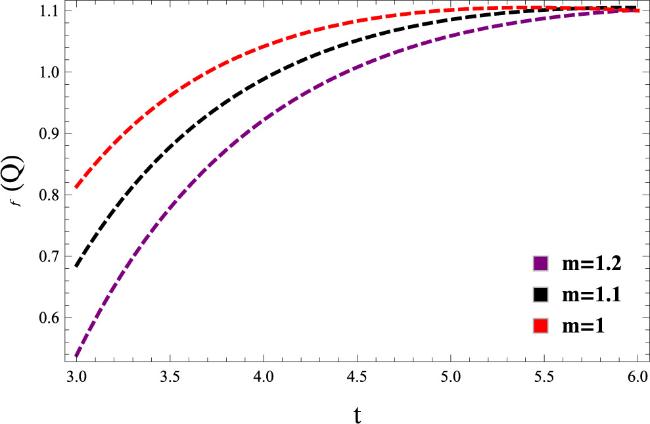
Throughout the graphical analysis, we assume a constant value of c = 0.5. Figure 1 illustrates that the reconstructed GDE model increases with respect to t while maintaining a positive value, which indicates a rapid expansion. Inserting equation (31) into (23) and (24), we obtain ρD and pD as
$\begin{eqnarray}\begin{array}{rc}{\rho }_{D} & =\,\frac{\alpha \sqrt{Q}}{\sqrt{6}}+c,\end{array}\end{eqnarray}$
$\begin{eqnarray}\begin{array}{rcl}{p}_{D} & = & \frac{1}{12{Q}^{\frac{3}{2}}}\left[c{Q}^{2}-4\dot{H}Q\left(\sqrt{6}\alpha -3c\right)\right.\\ & & +6\left({H}^{2}Q\left(6c-2\sqrt{6}\alpha \right)-cH\right)\\ & & \left.-\sqrt{6}\alpha \mathrm{ln}(Q)\left(Q(2\dot{H}+Q)+6{H}^{2}Q-H\right)\right].\end{array}\end{eqnarray}$
Using equation (28) into the above equations, we can express them in power-law form as
$\begin{eqnarray}\begin{array}{rc}{\rho }_{D} & =\alpha \sqrt{\frac{{m}^{2}}{{t}^{2}}}+c,\end{array}\end{eqnarray}$
$\begin{eqnarray}\begin{array}{rcl}{p}_{D} & = & \frac{1}{72\sqrt{6}{t}^{4}{\left(\frac{{m}^{2}}{{t}^{2}}\right)}^{3/2}}\\ & & \times \,\left[m\left(\sqrt{6}\alpha \left(-72{m}^{3}+12{m}^{2}+{t}^{3}\right)\mathrm{ln}\left(\frac{6{m}^{2}}{{t}^{2}}\right)\right.\right.\\ & & -\,6\left.\left.\left(12{m}^{3}(\sqrt{6}\alpha -6c)-4{m}^{2}(\sqrt{6}\alpha -3c)+c{t}^{3}\right)\right)\right].\end{array}\end{eqnarray}$
Figure 1. The graph illustrates the relationship between f(Q) and t.
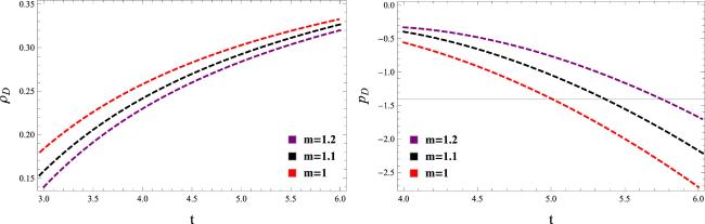
Figure 2 illustrates the behavior of ρD and pD. It is seen that the energy density ρD remains positive and exhibits an increasing pattern, consistent with the characteristics of DE, while pD demonstrates negative behavior with a decreasing trend. This positive energy density is not only stable but also increases over time, aligning with the theoretical expectations for DE models, where the energy density plays a crucial role in driving the accelerated expansion of the Universe. On the other hand, this negative pressure is necessary to explain the repulsive gravitational effect responsible for the Universe's accelerated expansion. The decreasing trend of pD in the graph highlights this behavior, reinforcing the idea that DE dominates over other forms of energy in the Universe at late times, causing the accelerated expansion.
Figure 2. Graphs show ρD and pD against t.
Now, we explore the evolution of the cosmos by conducting cosmographic analysis on the EoS parameter and phase planes for the GDE f(Q) model. We also discuss stability of this model by examining the squared sound speed. The EoS is defined as ${\omega }_{D}=\frac{{p}_{D}}{{\rho }_{D}},$ which is essential for determining the dynamics of expansion. Specific values of ωD correspond to distinct types of energy contributions to the Universe. For example, ωD = 0 indicates a matter-dominated region, typically associated with dust, while ${\omega }_{D}=\frac{1}{3}$ corresponds to radiation and ωD = 1 signifies stiff matter. In the context of DE, various ranges of ωD characterize different phases of expansion: ωD = −1 denotes a cosmological constant representing vacuum energy, ωD < −1 indicates the presence of phantom energy and $-1\lt {\omega }_{D}\lt -\tfrac{1}{3}$ represents quintessence. By analyzing the EoS parameter, researchers can gain insights into the dynamics of cosmic expansion and the nature of the Universe energy components. This can be evaluated as follows
$\begin{eqnarray}\begin{array}{rcl}{\omega }_{D} & = & \frac{1}{72\sqrt{6}\left(\alpha {m}^{3}\xi +m\sqrt{\frac{{m}^{2}}{{t}^{2}}}{t}^{2-3m}\right)}\\ & & \times \,\left[\xi \left(6\left(c\left(72{m}^{3}-12{m}^{2}-{t}^{3}\right)+4\sqrt{6}\right.\right.\right.\\ & & \times \left.\alpha (1-3m){m}^{2}\right)\\ & & +\,\left.\left.\sqrt{6}\alpha \left(-72{m}^{3}+12{m}^{2}+{t}^{3}\right)\mathrm{ln}\left(\frac{6{m}^{2}}{{t}^{2}}\right)\right)\right].\end{array}\end{eqnarray}$
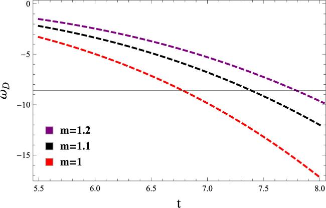
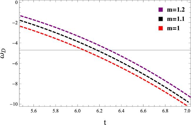
Figure 3 demonstrates the behavior of the EoS in GDE f(Q) gravity for three distinct values of m = 1.2, 1.1, 1, which represents ωD < −1, indicating the presence of phantom field DE. This suggests that the Universe is undergoing accelerated expansion at a rate faster than predicted by conventional models. Such expansion can significantly affect how the Universe evolves and may influence its ultimate fate. By analyzing the EoS for these values, it reveals the complex relationship between parameters in f(Q) gravity and DE, providing valuable insights into how modified gravity theories enhance our understanding of cosmic acceleration.
Figure 3. Plot shows the relationship between ωD with t.
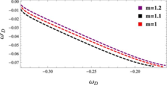
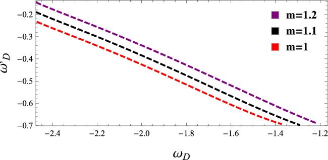
The (${\omega }_{D}-{\omega }_{D}^{{\prime} }$ )-plane [57] is used to study the dynamics and properties of DE models. Here ${\omega }_{D}^{{\prime} }$ represents its derivative with respect to Q. We classify the DE models into two distinct categories, i.e. thawing and freezing regions. When ωD < 0 and ${\omega }_{D}^{{\prime} }\gt 0,$ we have thawing region, while in the freezing region, ωD < 0 and ${\omega }_{D}^{{\prime} }\lt 0.$ Thus we have
$\begin{eqnarray}\begin{array}{rcl}{\omega }_{D}^{{\prime} } & = & \frac{1}{864\sqrt{6}{m}^{3}\sqrt{\frac{{m}^{2}}{{t}^{2}}}{\left(\alpha \xi \sqrt{\frac{{m}^{2}}{{t}^{2}}}{t}^{3m}+1\right)}^{2}}\\ & & \times \,\left[\xi {t}^{3m}\left(2\left(c\left(\left(2\alpha \xi \sqrt{\frac{{m}^{2}}{{t}^{2}}}{t}^{3m}+1\right)\right.\right.\right.\right.\\ & & \times \,36{m}^{2}+3{t}^{3}\left(4\alpha \xi \sqrt{\frac{{m}^{2}}{{t}^{2}}}{t}^{3m}+3\right)\\ & & -\,\left.216\alpha {m}^{3}\xi \sqrt{\frac{{m}^{2}}{{t}^{2}}}{t}^{3m}\right)\\ & & -\,\alpha \left(36{m}^{3}+12\alpha \xi {t}^{3m+2}{\left(\frac{{m}^{2}}{{t}^{2}}\right)}^{3/2}\right.\\ & & -\,\left.\left.{t}^{3}\left(\alpha \xi \sqrt{\frac{{m}^{2}}{{t}^{2}}}{t}^{3m}+1\right)\right)\sqrt{6}\right)+\alpha \mathrm{ln}\left(\frac{6{m}^{2}}{{t}^{2}}\right)\\ & & \times \,\sqrt{6}\left(-12{m}^{2}\left(2\alpha \xi \sqrt{\frac{{m}^{2}}{{t}^{2}}}{t}^{3m}+1\right)\right.\\ & & -\,{t}^{3}\left(4\alpha \xi \sqrt{\frac{{m}^{2}}{{t}^{2}}}{t}^{3m}+3\right)\\ & & +\,\left.\left.\left.\,72\alpha {m}^{3}\xi \sqrt{\frac{{m}^{2}}{{t}^{2}}}{t}^{3m}\right)\right)\right].\end{array}\end{eqnarray}$
Figure 4 illustrates that ${\omega }_{D}\lt 0,{\omega }_{D}^{{\prime} }\lt 0$ for various values of m, indicating the existence of the freezing region. This suggests that the acceleration of the cosmic expansion is increasing more significantly in this model.
Figure 4. Graph of ${\omega }_{D}^{{\prime} }$ against ωD.
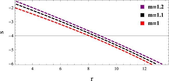
Statefinder parameters [58] are cosmological diagnostic tools used to characterize the expansion dynamics of the cosmos and distinguish between different DE models. One can identify specific trajectories that correspond to different DE models. Statefinder parameters thus provide valuable insights into the nature and behavior of DE, which help in comparing theoretical predictions with observational data. These can be described as [58]
$\begin{eqnarray*}r=\frac{\ddddot{a}}{a{H}^{3}},\quad s=\frac{r-1}{3(q-\frac{1}{2})}.\end{eqnarray*}$
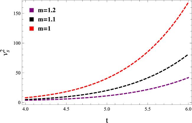
Trajectories within the range (r < 1) and (s > 0) correspond to phantom and quintessence DE eras, while trajectories with (r > 1) and (s < 0) indicate the Chaplygin gas model. The expressions for the (r − s) parameters are given in appendix A. Figure 5 indicates the Chaplygin gas model for three different values of m. This figure highlights how varying m affects the behavior of the Chaplygin gas model, which is characterized by a unified description of DE and DM. The results presented in this figure demonstrate the versatility of the Chaplygin gas model in explaining the accelerated expansion of the Universe while simultaneously offering insights into the interactions between DE and modified gravity in the f(Q) framework. The squared speed of sound plays a crucial role to analyze the stability of different models. In the DE models, when ${\nu }_{s}^{2}$ is positive it characterizes the stability while a negative ${\nu }_{s}^{2}$ leads to instability. The corresponding ${\nu }_{s}^{2}$ is given as
$\begin{eqnarray}\begin{array}{rcl}{\nu }_{s}^{2} & = & \frac{1}{5184\sqrt{6}\alpha {m}^{6}{\left(\alpha \xi \sqrt{\frac{{m}^{2}}{{t}^{2}}}{t}^{3m}+1\right)}^{2}}\\ & & \times \,\left[\xi \sqrt{\frac{{m}^{2}}{{t}^{2}}}{t}^{3m}\left(6\left(12{m}^{3}\left(\sqrt{6}\alpha -6c\right)\right.\right.\right.\\ & & -\,\left.4{m}^{2}\left(\sqrt{6}\alpha -3c\right)+c{t}^{3}\right)\\ & & +\,\left.\sqrt{6}\alpha \left(72{m}^{3}-12{m}^{2}-{t}^{3}\right)\mathrm{ln}\left(\frac{6{m}^{2}}{{t}^{2}}\right)\right)\\ & & \times \,\left(-24\alpha (3m-1)\xi \left(\alpha -\sqrt{6}c\right){t}^{3m+2}{\left(\frac{{m}^{2}}{{t}^{2}}\right)}^{\frac{3}{2}}\right.\\ & & -\,2\alpha \xi \left(\alpha +2\sqrt{6}c\right){t}^{3m+3}\\ & & \times \,\sqrt{\frac{{m}^{2}}{{t}^{2}}}-12\sqrt{6}c{m}^{2}-{t}^{3}\left(2\alpha +3\sqrt{6}c\right)\\ & & -\,\alpha \mathrm{ln}\left(\frac{6{m}^{2}}{{t}^{2}}\right)\left(1-\left(2\alpha \xi {t}^{3m}\sqrt{\frac{{m}^{2}}{{t}^{2}}}\right)12{m}^{2}\right.\\ & & -\,{t}^{3}\left(4\alpha \xi \sqrt{\frac{{m}^{2}}{{t}^{2}}}{t}^{3m}+3\right)\\ & & \left.\left.\left.+\,72\alpha {m}^{3}\xi \sqrt{\frac{{m}^{2}}{{t}^{2}}}{t}^{3m}\right)\right)\right].\end{array}\end{eqnarray}$
Figure 5. Graph depicts r against s.
Figure 6 illustrates a consistently decreasing trend of ${\nu }_{s}^{2},$ indicating the instability of the GDE model for various values of m. This downward trend is important because it indicates possible instability in the GDE framework. When ${\nu }_{s}^{2}$ gets very low or negative, it means the model might not behave as expected, which can affect its ability to explain how the Universe evolves. Understanding a stable DE model is crucial for studying the Universe's expansion. The results in this figure highlight the challenges faced by the GDE model, suggesting the need for further research on how different values of m impact stability. It is essential to explore changes to DE theories to ensure they provide reliable descriptions of cosmic acceleration.
Figure 6. Graph of ${\nu }_{s}^{2}$ with t.

4. Reconstruction of GGDE f(Q) model

In this section, we reconstruct the GGDE f(Q) model by equating the corresponding densities equal to each other. Applying equations (2) and (23), it is demonstrated that
$\begin{eqnarray}\frac{f}{2}-6{H}^{2}{f}_{Q}=\alpha H+\beta {H}^{2}.\end{eqnarray}$
Its solution is given by
$\begin{eqnarray}f(Q)=-\frac{1}{6}\sqrt{Q}\left(-6c+\sqrt{6}\alpha \mathrm{ln}(Q)+2\beta \sqrt{Q}\right),\end{eqnarray}$
and in terms of t, we have
$\begin{eqnarray}\begin{array}{rcl}f(Q) & = & \sqrt{6}c\sqrt{\frac{{m}^{2}}{{t}^{2}}}-\alpha \sqrt{\frac{{m}^{2}}{{t}^{2}}}\\ & & \times \,\mathrm{ln}\left(\frac{6{m}^{2}}{{t}^{2}}\right)-\frac{2\beta {m}^{2}}{{t}^{2}}.\end{array}\end{eqnarray}$
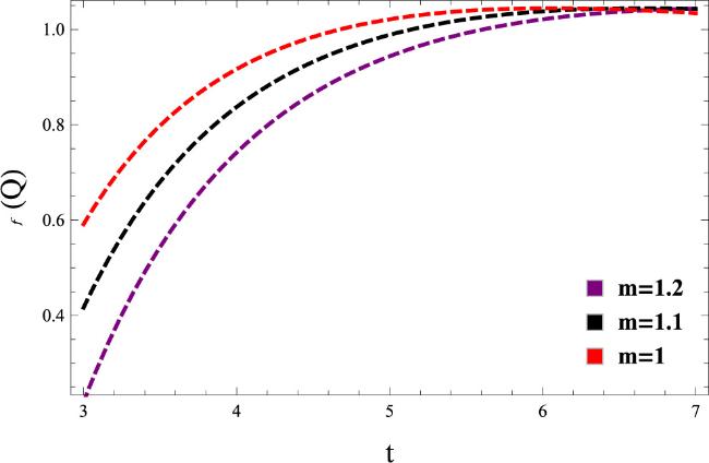
Figure 7 demonstrates that the reconstructed GGDE model exhibits an increasing behavior with time, while maintaining a consistently positive value. This observation implies that the GGDE model indicates an accelerated expansion of the Universe. Using equation (41) in (23) and (24), we have
$\begin{eqnarray}{\rho }_{D}=\frac{1}{6}\left(\sqrt{6}\alpha \sqrt{Q}+\beta Q\right)+c,\end{eqnarray}$
$\begin{eqnarray}\begin{array}{rcl}{p}_{D} & = & \frac{1}{12{Q}^{\frac{3}{2}}}\left[-2\left(3cH-3c{Q}^{2}\right.\right.\\ & & +\,\left(\sqrt{6}\alpha -3c+2\beta \sqrt{Q}\right)\left(2\dot{H}Q+6{H}^{2}Q\right)\\ & & +\,\left.\left.\beta {Q}^{\frac{5}{2}}\right)-\sqrt{6}\alpha \mathrm{ln}Q\left(Q(2\dot{H}+Q)+6{H}^{2}Q-H\right)\right].\end{array}\end{eqnarray}$
Substituting equation (28) into the above equations, we can express them in power-law form as
$\begin{eqnarray}{\rho }_{D}=\alpha \sqrt{\frac{{m}^{2}}{{t}^{2}}}+\frac{\beta {m}^{2}}{{t}^{2}}+c,\end{eqnarray}$
$\begin{eqnarray}\begin{array}{rcl}{p}_{D} & = & \frac{1}{72\sqrt{6}{t}^{4}{\left(\frac{{m}^{2}}{{t}^{2}}\right)}^{\frac{3}{2}}}\left[m\left(\sqrt{6}\alpha \left(12{m}^{2}-72{m}^{3}+{t}^{3}\right)\right.\right.\\ & & \times \mathrm{ln}\left(\frac{6{m}^{2}}{{t}^{2}}\right)-\,6\left(c{t}^{3}+\left(\sqrt{6}\alpha -3c+2\sqrt{6}\beta \sqrt{\frac{{m}^{2}}{{t}^{2}}}\right)\right.\\ & & \left.\left.\left.\times (12{m}^{3}-4{m}^{2})\right)\right)\right].\end{array}\end{eqnarray}$
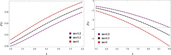
Figure 8 shows the decreasing trend of pD, while ρD maintains positivity and increases steadily. These patterns align with the expected behavior of DE contributing to the understanding of cosmic acceleration. The corresponding EoS parameter takes the form
$\begin{eqnarray}\begin{array}{rcl}{\omega }_{D} & = & -\left\{{t}^{3m}\left(6\left(-4{m}^{2}\left(\sqrt{6}\alpha -3c+2\sqrt{6}\beta \sqrt{\frac{{m}^{2}}{{t}^{2}}}\right)\right.\right.\right.\\ & & +\,\left.12{m}^{3}\left(\sqrt{6}\alpha -6c+3\sqrt{6}\beta \sqrt{\frac{{m}^{2}}{{t}^{2}}}\right)+c{t}^{3}\right)\\ & & +\,\left.\left.\sqrt{6}\alpha \left(72{m}^{3}-12{m}^{2}-{t}^{3}\right)\mathrm{ln}\left(\frac{6{m}^{2}}{{t}^{2}}\right)\right)\right\}\\ & & \times \,{\left\{72\sqrt{6}m\sqrt{\frac{{m}^{2}}{{t}^{2}}}\left(\beta {m}^{2}{t}^{3m}+\alpha \sqrt{\frac{{m}^{2}}{{t}^{2}}}{t}^{3m+2}+\xi {t}^{2}\right)\right\}}^{-1}.\end{array}\end{eqnarray}$
Figure 7. Graphical representation of f(Q) versus t.
Figure 8. Plots of ρD and pD versus t.
Figure 9 shows the presence of a phantom epoch during both the current and late-time cosmic evolution for various values of m. The significance of a phantom epoch lies in its implications for the dynamics of the Universe’s expansion. During this phase, the energy density associated with DE increases, leading to an accelerated expansion rate that exceeds predictions made by standard cosmological models. This behavior raises the possibility of a future cosmic event where the Universe’s expansion accelerates to a point that could disrupt the fabric of spacetime. Overall, this figure highlights the complex behavior of DE and underscores the importance of exploring how modifications to existing models can improve our understanding of cosmic evolution.
Figure 9. Graph of ωD with t.
The expression of ${\omega }_{D}^{{\prime} }$ is given as
$\begin{eqnarray}\begin{array}{rcl}{\omega }_{D}^{{\prime} } & = & \left\{\sqrt{\frac{{m}^{2}}{{t}^{2}}}{t}^{3m+4}\left(\frac{1}{{m}^{2}}\left[2\sqrt{\frac{{m}^{2}}{{t}^{2}}}\left(\xi {t}^{7}\left(\sqrt{6}\alpha +9c\right)\sqrt{\frac{{m}^{2}}{{t}^{2}}}\right.\right.\right.\right.\\ & & +\,{m}^{2}{t}^{4}\left(36c\xi \sqrt{\frac{{m}^{2}}{{t}^{2}}}+{t}^{3m+1}\left(\sqrt{6}{\alpha }^{2}\right.\right.\\ & & +\,\left.\left.12\alpha c+15\beta c\sqrt{\frac{{m}^{2}}{{t}^{2}}}+\sqrt{6}\alpha \beta \sqrt{\frac{{m}^{2}}{{t}^{2}}}\right)\right)\\ & & +\,72{m}^{5}{t}^{2}\left({t}^{3m}\left(-3\alpha c-6\beta c\sqrt{\frac{{m}^{2}}{{t}^{2}}}\right.\right.\\ & & \left.\left.+\sqrt{6}\alpha \beta \sqrt{\frac{{m}^{2}}{{t}^{2}}}\right)-\sqrt{6}\beta \xi \right)\\ & & -\,12{m}^{4}{t}^{3m+2}\left(\sqrt{6}{\alpha }^{2}-6\alpha c-9\beta c\sqrt{\frac{{m}^{2}}{{t}^{2}}}\right.\\ & & \left.+4\sqrt{6}\alpha \beta \sqrt{\frac{{m}^{2}}{{t}^{2}}}\right)\\ & & +\,144\sqrt{6}{\beta }^{2}{m}^{7}{t}^{3m}-48\sqrt{6}{\beta }^{2}{m}^{6}{t}^{3m}\\ & & -\left.\left.\,36\sqrt{6}\alpha m\xi {t}^{6}{\left(\frac{{m}^{2}}{{t}^{2}}\right)}^{3/2}\right)\right]\\ & & +\,\sqrt{6}\alpha \mathrm{ln}\left(\frac{6{m}^{2}}{{t}^{2}}\right)\left(144\beta {m}^{5}{t}^{3m}-36\beta {m}^{4}{t}^{3m}\right.\\ & & -\,{m}^{2}{t}^{2}\left(24\alpha \sqrt{\frac{{m}^{2}}{{t}^{2}}}{t}^{3m}+5\beta {t}^{3m+1}+12\xi \right)\\ & & -\,{t}^{5}\left(4\alpha \sqrt{\frac{{m}^{2}}{{t}^{2}}}{t}^{3m}+3\xi \right)\\ & & +\,\left.\left.\left.\frac{\alpha {m}^{5}{t}^{3m}}{\sqrt{\frac{{m}^{2}}{{t}^{2}}}}\right)\right)\right\}\left\{864\sqrt{6}{m}^{5}\left(\beta {m}^{2}{t}^{3m}\right.\right.\\ & & +\,{\left.{\left.\alpha \sqrt{\frac{{m}^{2}}{{t}^{2}}}{t}^{3m+2}+\xi {t}^{2}\right)}^{2}\right\}}^{-1}.\end{array}\end{eqnarray}$
Figure 10 demonstrates the cosmic trajectories on the ${\omega }_{D}-{\omega }_{D}^{{\prime} }$ plane for certain values of m, illustrating the freezing region of the Universe. This plane represents the current cosmic expansion paradigm, where the freezing region suggests a phase of accelerated expansion compared to the thawing region. This behavior is crucial as it suggests that the universe may experience a stable acceleration in its expansion over time. By analyzing the trajectories for various values of m, this figure provides insights into how modifications to the GGDE model influence cosmic evolution. Each trajectory illustrates how changes in m can affect the relationship between ωD and its derivative ${\omega }_{D}^{{\prime} },$ revealing patterns that characterize the interaction between DE and cosmic expansion. Overall, this figure serves as a vital tool for exploring the dynamics of DE and its implications for the evolution of the universe, emphasizing the significance of the freezing region in understanding cosmic acceleration.
Figure 10. Plot of ${\omega }_{D}^{{\prime} }$ versus ωD.
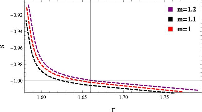
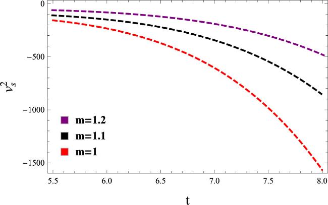
The (rs)-plane is given in appendix B. Figure 11 depicts the graphical examination of the rs plane. This shows that r > 1 and s < 0, indicating the presence of the Chaplygin gas model. The expression for ${\nu }_{s}^{2}$ is provided as follows
$\begin{eqnarray*}\begin{array}{rcl}{\nu }_{s}^{2} & = & -\left\{{t}^{3m}\left(6\left(c{t}^{3}-4{m}^{2}\left(\sqrt{6}\alpha -3c+2\sqrt{6}\beta \sqrt{\frac{{m}^{2}}{{t}^{2}}}\right)\right.\right.\right.\\ & & +\,\left.12{m}^{3}\left(\sqrt{6}\alpha -6c+\,3\sqrt{6}\beta \sqrt{\frac{{m}^{2}}{{t}^{2}}}\right)\right)\\ & & +\,\left.\sqrt{6}\alpha \left(72{m}^{3}-12{m}^{2}-{t}^{3}\right)\mathrm{ln}\left(\frac{6{m}^{2}}{{t}^{2}}\right)\right)\\ & & \times \left(\frac{1}{{m}^{2}}\left[2\sqrt{\frac{{m}^{2}}{{t}^{2}}}\right.\right.\left(\xi {t}^{7}\left(\sqrt{6}\alpha +9c\right)\sqrt{\frac{{m}^{2}}{{t}^{2}}}\right.\\ & & +\,{m}^{2}{t}^{4}\left(36c\xi \sqrt{\frac{{m}^{2}}{{t}^{2}}}+{t}^{3m+1}\left(\sqrt{6}{\alpha }^{2}+12\alpha c\right.\right.\end{array}\end{eqnarray*}$
$\begin{eqnarray*}\begin{array}{rcl} & & +\,\left.\left.15\beta c\sqrt{\frac{{m}^{2}}{{t}^{2}}}+\sqrt{6}\alpha \beta \sqrt{\frac{{m}^{2}}{{t}^{2}}}\right)\right)\\ & & +\,36{t}^{3m+2}\left(\sqrt{6}{\alpha }^{2}-6\alpha c-12\beta c\sqrt{\frac{{m}^{2}}{{t}^{2}}}\right.\\ & & +\,5\left.\sqrt{6}\alpha \beta \sqrt{\frac{{m}^{2}}{{t}^{2}}}\right){m}^{5}-12{m}^{4}{t}^{3m+2}\left(\sqrt{6}{\alpha }^{2}\right.\\ & & -\,6\alpha c-9\beta c\sqrt{\frac{{m}^{2}}{{t}^{2}}}+4\sqrt{6}\alpha \beta \\ & & \times \,\left.\left.\left.\sqrt{\frac{{m}^{2}}{{t}^{2}}}\right)+216\sqrt{6}{\beta }^{2}{m}^{7}{t}^{3m}-48\sqrt{6}{\beta }^{2}{m}^{6}{t}^{3m}\right)\right]\\ & & +\,\sqrt{6}\alpha \mathrm{ln}\left(\frac{6{m}^{2}}{{t}^{2}}\right)\end{array}\end{eqnarray*}$
$\begin{eqnarray}\begin{array}{rcl} & & \times \,\left(144\beta {m}^{5}{t}^{3m}-36\beta {m}^{4}{t}^{3m}\right.\\ & & -\,{m}^{2}{t}^{2}\left(24\alpha \sqrt{\frac{{m}^{2}}{{t}^{2}}}{t}^{3m}+5\beta {t}^{3m+1}+12\xi \right)\\ & & -\,{t}^{5}\left(4\alpha \sqrt{\frac{{m}^{2}}{{t}^{2}}}{t}^{3m}+3\xi \right)\\ & & +\,\left.\left.\left.\frac{72\alpha {m}^{5}{t}^{3m}}{\sqrt{\frac{{m}^{2}}{{t}^{2}}}}\right)\right)\right\}\left\{31104{m}^{4}\left(\alpha +2\beta \sqrt{\frac{{m}^{2}}{{t}^{2}}}\right)\right.\\ & & \times \,{\left.\sqrt{\frac{{m}^{2}}{{t}^{2}}}{\left(\beta {m}^{2}{t}^{3m}+\alpha \sqrt{\frac{{m}^{2}}{{t}^{2}}}{t}^{3m+2}+\xi {t}^{2}\right)}^{2}\right\}}^{-1}.\end{array}\end{eqnarray}$
Figure 12 demonstrates that the squared speed of sound is positive for all considered values of m which indicates the model is stable.
Figure 11. Plot of r versus s.
Figure 12. Graph of ${\nu }_{s}^{2}$ versus t.

5. Conclusions

The main goal of this manuscript is to achieve a comprehensive understanding of the cosmic behavior and consequences of DE models in the framework of cosmic evolution. Initially, we have reconstructed the DE f(Q) gravity models using the correspondence scheme which serves as a fundamental approach in constructing DE models. We have employed the FRW model with a power-law scale factor to investigate the non-interacting scenario. Our analysis has delved into the exploration of the evolution trajectories of the EoS parameter. We have extensively investigated the $({\omega }_{D}-{\omega }_{D}^{{\prime} })$ and (rs)-planes which offer valuable insights into the phase space dynamics of the GDE and GGDE models. The main findings are summarized as follows.

• For various values of m, the resulting f(Q) gravity of both DE models indicate an increasing trend over time, indicating that the reconstructed models are realistic (figures 1 and 7).

• Both DE models show an increasing trend for energy density, while the pressure shows consistently negative characteristic for all values of m. This behavior is consistent with the typical features of DE (figures 2 and 8).

• The EoS indicates the existence of phantom field DE in both models. This parameter becomes more negative below −1 which is consistent with the current understanding of accelerated cosmic expansion (figures 3 and 9).

• The freezing area for all values of m is depicted by the evolutionary behavior in the (ωD${\omega }_{D}^{{\prime} }$ )-plane. This observation provides confirmation that the non-interacting GGD and GGDE f(Q) gravity models suggest a more rapid expansion of the Universe (figures 4 and 10).

• For both models, the (rs)-plane depicts the Chaplygin gas model for various values of m (figures 5 and 11).

• It is found that ${\nu }_{s}^{2}\lt 0$ for the GDE f(Q) gravity model indicating the instability (figure 6) but ${\nu }_{s}^{2}\gt 0$ for the GGDE f(Q) gravity model, suggesting stability across all values of m (figure 12).

We have observed that the findings align with the observational data [59] as indicated
$\begin{eqnarray*}\begin{array}{rcl}{\omega }_{D} & = & -1.02{3}_{-0.096}^{+0.091}\quad (\,\rm{Planck TT+LowP+ext}\,),\\ {\omega }_{D} & = & -1.00{6}_{-0.091}^{+0.085}\quad (\,\rm{Planck TT+LowP+lensing+ext}\,),\\ {\omega }_{D} & = & -1.01{9}_{-0.080}^{+0.075}\quad (\,\rm{Planck TT, TE, EE+LowP+ext}\,).\end{array}\end{eqnarray*}$
These values have been determined reaching a confidence level of 85%. Notably, the EoS in the GGDE model exhibits a closer alignment with observational data as compared to that of the GDE model. Our results are consistent with the most recent theoretical observational findings [33, 52, 59].
We have noted that the results obtained from both the reconstruction scheme in non-interacting ghost dark energy GDE and generalized ghost dark energy GGDE align with modern observational data, as well as with the studies conducted by [22]–[24] Additionally, Malekjani [60] used the GGDE model to explore the current cosmic expansion, both with and without interaction terms, to study its cosmological evolution. Zubair and Abbas [61] developed the $f(R,{\mathbb{T}})$ gravity using the GDE model in a flat FRW universe and found that their model includes both phantom and quintessential phases. Myrzakulov et al [62] examined the connection between f(Q) and the GDE model, finding that the EoS parameter crosses the phantom divide line. Our results align with these findings. While this approach captures certain elements of the early universe dynamics, it does not take into account non-metricity. By including Q in the model, we address both early and late-time cosmic acceleration, providing a more complete picture of the Universe evolution. Comparing the results of the f(Q) gravity model with these other theories, we show that this method offers an observationally consistent model of the Universe accelerated expansion, contributing to a better understanding of DE and cosmic evolution.

Appendix A Calculation of r and s in GDE

$\begin{eqnarray*}\begin{array}{rcl}r & = & \frac{1}{768{m}^{10}{\left(6\sqrt{\frac{{m}^{2}}{{t}^{2}}}\alpha \xi {t}^{3m}+6\right)}^{4}}\\ & & \times \,\left[24\sqrt{6}{t}^{3m+5}\xi \left(\sqrt{\frac{{m}^{2}}{{t}^{2}}}\alpha \xi {t}^{3m}+1\right)\right.\\ & & \times \,\left(2\left(-c864{m}^{5}{\alpha }^{2}{\xi }^{2}{t}^{6m}-24{m}^{4}{\alpha }^{2}{\xi }^{2}\left(\sqrt{6}\alpha -12c\right){t}^{6m}\right.\right.\\ & & +\,\left(18\sqrt{6}\sqrt{\frac{{m}^{2}}{{t}^{2}}}{\alpha }^{2}\xi {t}^{3m}\right.\\ & & +\,\left.111\sqrt{\frac{{m}^{2}}{{t}^{2}}}\alpha \xi c{t}^{3m}+8\sqrt{6}\alpha +45c\right){t}^{5}\\ & & -\,\left(3\sqrt{\frac{{m}^{2}}{{t}^{2}}}\alpha \xi {t}^{3m}+1\right)\left(\sqrt{6}\alpha +6c\right)\\ & & \times \,36{m}^{3}{t}^{2}+2{m}^{2}\left(6{\alpha }^{2}\xi \left(6\xi c{t}^{3m+1}+\sqrt{6}\sqrt{\frac{{m}^{2}}{{t}^{2}}}\right){t}^{3m}\right.\\ & & +\,5\sqrt{6}{\alpha }^{3}{\xi }^{2}{t}^{6m+1}+54c\end{array}\end{eqnarray*}$
$\begin{eqnarray*}\begin{array}{rcl} & & +\,6\alpha \left.\left.\left(27\sqrt{\frac{{m}^{2}}{{t}^{2}}}\xi c{t}^{3m}+\sqrt{6}\right)\right){t}^{2}\right)\\ & & +\,\sqrt{6}\alpha \left(288{m}^{5}{\alpha }^{2}{\xi }^{2}{t}^{6m}-96{m}^{4}{\alpha }^{2}{\xi }^{2}{t}^{6m}\right.\\ & & -\,\left(37\sqrt{\frac{{m}^{2}}{{t}^{2}}}\alpha \xi {t}^{3m}+15\right){t}^{5}\\ & & +\,72{m}^{3}\left(3\sqrt{\frac{{m}^{2}}{{t}^{2}}}\alpha \xi {t}^{3m}+1\right){t}^{2}\\ & & -\,\left.12{m}^{2}\left(9\alpha \xi \sqrt{\frac{{m}^{2}}{{t}^{2}}}{t}^{3m}+2{\alpha }^{2}{\xi }^{2}{t}^{6m+1}+3\right){t}^{2}\right)\\ & & \times \left.\mathrm{ln}\left(\frac{6{m}^{2}}{{t}^{2}}\right)\right){\left(\frac{{m}^{2}}{{t}^{2}}\right)}^{3/2}+\left(\sqrt{6}{t}^{3m}\alpha \xi \right.\\ & & \times \,\left(24{m}^{4}\alpha \xi {t}^{3m}-72{m}^{5}\alpha \xi {t}^{3m}+3\sqrt{\frac{{m}^{2}}{{t}^{2}}}{t}^{5}\right.\end{array}\end{eqnarray*}$
$\begin{eqnarray*}\begin{array}{rcl} & & +\,\left.\left(\alpha \xi {t}^{3m+1}+3\sqrt{\frac{{m}^{2}}{{t}^{2}}}\right){t}^{2}4{m}^{2}\right)\\ & & \times \mathrm{ln}\left(\frac{6{m}^{2}}{{t}^{2}}\right)-2\left(-\frac{36\sqrt{6}{m}^{5}\alpha \xi {t}^{3m}}{\sqrt{\frac{{m}^{2}}{{t}^{2}}}}\right.\\ & & -\,12{m}^{4}\alpha {\xi }^{2}\left(\sqrt{6}\alpha -6c\right){t}^{6m}+{m}^{2}\xi \\ & & \times \,\left(\alpha \xi \left(\sqrt{6}\alpha +12c\right){t}^{3m+1}+36\sqrt{\frac{{m}^{2}}{{t}^{2}}}c\right){t}^{3m+2}\\ & & +\,\sqrt{\frac{{m}^{2}}{{t}^{2}}}\xi \left(\sqrt{6}\alpha +9c\right){t}^{3m+5}\\ & & +\,144\sqrt{6}{m}^{7}{\alpha }^{2}{\xi }^{2}{t}^{6m-2}\\ & & +\,{\left.\left.72{m}^{5}\left(4\sqrt{6}\sqrt{\frac{{m}^{2}}{{t}^{2}}}\alpha \xi {t}^{3m}-3\alpha {\xi }^{2}c{t}^{6m}+2\sqrt{6}\right)\right)\right)}^{2}\end{array}\end{eqnarray*}$
$\begin{eqnarray*}\begin{array}{rcl} & & +\,288\sqrt{6}{m}^{5}{\left(\sqrt{\frac{{m}^{2}}{{t}^{2}}}\alpha \xi {t}^{3m}+1\right)}^{2}\\ & & \times \,\left(2\left(-\frac{36\sqrt{6}{m}^{5}\alpha \xi {t}^{3m}}{\sqrt{\frac{{m}^{2}}{{t}^{2}}}}-12{m}^{4}\alpha {\xi }^{2}{t}^{6m}\right.\right.\\ & & \times \,\left(\sqrt{6}\alpha -6c\right)+{m}^{2}\xi \left(\alpha \xi \left(\sqrt{6}\alpha +12c\right){t}^{3m+1}\right.\\ & & +\,36\left.\sqrt{\frac{{m}^{2}}{{t}^{2}}}c\right){t}^{3m+2}+\sqrt{\frac{{m}^{2}}{{t}^{2}}}\\ & & \times \xi \left(\sqrt{6}\alpha +9c\right){t}^{3m+5}+144\sqrt{6}{m}^{7}{\alpha }^{2}{\xi }^{2}{t}^{6m-2}\\ & & +\,72{m}^{5}\left(4\sqrt{6}\sqrt{\frac{{m}^{2}}{{t}^{2}}}\alpha \xi {t}^{3m}\right.\\ & & -\,\left.\left.3\alpha {\xi }^{2}c{t}^{6m}+2\sqrt{6}\right)\right)\\ & & -\,\sqrt{6}{t}^{3m}\xi \left(24{m}^{4}\alpha \xi {t}^{3m}-72{m}^{5}\alpha \xi {t}^{3m}+3\sqrt{\frac{{m}^{2}}{{t}^{2}}}{t}^{5}\right.\\ & & +\,\left.\left.\left.4{m}^{2}\left(\alpha \xi {t}^{3m+1}+3\sqrt{\frac{{m}^{2}}{{t}^{2}}}\right){t}^{2}\right)\alpha \mathrm{ln}\left(\frac{6{m}^{2}}{{t}^{2}}\right)\right)\right],\end{array}\end{eqnarray*}$
$\begin{eqnarray*}\begin{array}{rcl}s & = & -\left\{16\sqrt{\frac{2}{3}}m{\left(\frac{{m}^{2}}{{t}^{2}}\right)}^{3/2}{t}^{2-3m}{\left(6\sqrt{\frac{{m}^{2}}{{t}^{2}}}\alpha \xi {t}^{3m}+6\right)}^{2}\right.\\ & & \times \,\left(\left[\left(\sqrt{\frac{{m}^{2}}{{t}^{2}}}\alpha \xi {t}^{3m}+1\right)\right.\right.\\ & & \times \,24\sqrt{6}{t}^{3m+5}\xi \left(2\left(-864{m}^{5}{\alpha }^{2}{\xi }^{2}c{t}^{6m}\right.\right.\\ & & -\,24{m}^{4}{\alpha }^{2}{\xi }^{2}\left(\sqrt{6}\alpha -12c\right){t}^{6m}\\ & & \times \left(45c+18\sqrt{6}\sqrt{\frac{{m}^{2}}{{t}^{2}}}{\alpha }^{2}\xi {t}^{3m}\right.\\ & & +\,\left.111\sqrt{\frac{{m}^{2}}{{t}^{2}}}\alpha \xi c{t}^{3m}+8\sqrt{6}\alpha \right){t}^{5}\\ & & -\left(\sqrt{6}\alpha +6c\right)36{m}^{3}\\ & & \times \,\left(3\sqrt{\frac{{m}^{2}}{{t}^{2}}}\alpha \xi {t}^{3m}+1\right){t}^{2}\end{array}\end{eqnarray*}$
$\begin{eqnarray*}\begin{array}{rcl} & & +\,2{m}^{2}\left(6{\alpha }^{2}\xi \left(6\xi c{t}^{3m+1}+\sqrt{6}\sqrt{\frac{{m}^{2}}{{t}^{2}}}\right){t}^{3m}+54c\right.\\ & & +\,\left.\left.5\sqrt{6}{\alpha }^{3}{\xi }^{2}{t}^{6m+1}+6\alpha \left(27\sqrt{\frac{{m}^{2}}{{t}^{2}}}\xi c{t}^{3m}+\sqrt{6}\right)\right){t}^{2}\right)\\ & & +\,\left(288{m}^{5}{\alpha }^{2}{\xi }^{2}{t}^{6m}-96{m}^{4}{\alpha }^{2}{\xi }^{2}{t}^{6m}\right.\\ & & -\,\left(37\sqrt{\frac{{m}^{2}}{{t}^{2}}}\alpha \xi {t}^{3m}+15\right){t}^{5}\\ & & +\,72{m}^{3}\left(3\sqrt{\frac{{m}^{2}}{{t}^{2}}}\alpha \xi {t}^{3m}+1\right){t}^{2}\\ & & -\,12{m}^{2}\left.\left(9\sqrt{\frac{{m}^{2}}{{t}^{2}}}\alpha \xi {t}^{3m}+2{\alpha }^{2}{\xi }^{2}{t}^{6m+1}+3\right){t}^{2}\right)\\ & & \times \,\left.\sqrt{6}\alpha \mathrm{ln}\left(\frac{6{m}^{2}}{{t}^{2}}\right)\right){\left(\frac{{m}^{2}}{{t}^{2}}\right)}^{3/2}\end{array}\end{eqnarray*}$
$\begin{eqnarray*}\begin{array}{rcl} & & +\,\left(\sqrt{6}{t}^{3m}\alpha \xi \left(-72{m}^{5}\alpha \xi {t}^{3m}+24{m}^{4}\alpha \xi {t}^{3m}\right.\right.\\ & & +\,3\sqrt{\frac{{m}^{2}}{{t}^{2}}}{t}^{5}+4{m}^{2}\left(\alpha \xi {t}^{3m+1}\right.\\ & & +\,3\left.\left.\sqrt{\frac{{m}^{2}}{{t}^{2}}}\right){t}^{2}\right)\mathrm{ln}\left(\frac{6{m}^{2}}{{t}^{2}}\right)\\ & & -\,2\left(-\frac{36\sqrt{6}{m}^{5}\alpha \xi {t}^{3m}}{\sqrt{\frac{{m}^{2}}{{t}^{2}}}}-12{m}^{4}\alpha {\xi }^{2}\left(\sqrt{6}\alpha -6c\right)\right.\\ & & \times \,{t}^{6m}+{m}^{2}\xi \left(\alpha \xi \left(\sqrt{6}\alpha +12c\right){t}^{3m+1}+36\sqrt{\frac{{m}^{2}}{{t}^{2}}}c\right){t}^{3m+2}\\ & & +\,\left(\sqrt{6}\alpha +9c\right)\xi \\ & & \times \,\sqrt{\frac{{m}^{2}}{{t}^{2}}}{t}^{3m+5}+144\sqrt{6}{m}^{7}{\alpha }^{2}{\xi }^{2}{t}^{6m-2}\end{array}\end{eqnarray*}$
$\begin{eqnarray*}\begin{array}{rcl} & & +\,72{m}^{5}\left(4\sqrt{6}\sqrt{\frac{{m}^{2}}{{t}^{2}}}\alpha \xi {t}^{3m}+2\sqrt{6}\right.\\ & & -\,{\left.\left.\left.3\alpha {\xi }^{2}c{t}^{6m}\right)\right)\right)}^{2}+288\sqrt{6}{m}^{5}{\left(\sqrt{\frac{{m}^{2}}{{t}^{2}}}\alpha \xi {t}^{3m}+1\right)}^{2}\\ & & \times \left(2\left(-\frac{36\sqrt{6}{m}^{5}\alpha \xi {t}^{3m}}{\sqrt{\frac{{m}^{2}}{{t}^{2}}}}\right.\right.\end{array}\end{eqnarray*}$
$\begin{eqnarray*}\begin{array}{rcl} & & -\,12{m}^{4}\alpha {\xi }^{2}\left(\sqrt{6}\alpha -6c\right){t}^{6m}+{m}^{2}\xi \left(\alpha \left(\sqrt{6}\alpha \right.\right.\\ & & \left.+12c\right){t}^{3m+1}\\ & & +\,36\left.\sqrt{\frac{{m}^{2}}{{t}^{2}}}c\right){t}^{3m+2}\\ & & +\,\sqrt{\frac{{m}^{2}}{{t}^{2}}}\xi \left(\sqrt{6}\alpha +9c\right){t}^{3m+5}+144\sqrt{6}{m}^{7}{\alpha }^{2}{\xi }^{2}{t}^{6m-2}\\ & & +\,\left(4\sqrt{6}\sqrt{\frac{{m}^{2}}{{t}^{2}}}\alpha \xi {t}^{3m}\right.\\ & & -\,\left.\left.3\alpha {\xi }^{2}c{t}^{6m}+2\sqrt{6}\right)72{m}^{5}\right)\\ & & -\,\sqrt{6}{t}^{3m}\alpha \xi \left(24{m}^{4}\alpha \xi {t}^{3m}-72{m}^{5}\alpha \xi {t}^{3m}+{t}^{5}\right.\\ & & \times \left.\left.\left.3\sqrt{\frac{{m}^{2}}{{t}^{2}}}+4{m}^{2}\left(\alpha \xi {t}^{3m+1}+3\sqrt{\frac{{m}^{2}}{{t}^{2}}}\right){t}^{2}\right)\mathrm{ln}\left(\frac{6{m}^{2}}{{t}^{2}}\right)\right)\right]\\ & & \times \,\left[768{m}^{10}\left(6\sqrt{\frac{{m}^{2}}{{t}^{2}}}\right.\right.\\ & & \times \left.\left.{\left.{\left.\alpha \xi {t}^{3m}+6\right)}^{4}\right]}^{-1}-1\right)\right\}\left\{\xi \left(2\left(36\alpha \left(6\sqrt{\frac{{m}^{2}}{{t}^{2}}}\xi c{t}^{3m}\right.\right.\right.\right.\\ & & \left.+\sqrt{6}\right){m}^{3}\\ & & +\left(\sqrt{\frac{{m}^{2}}{{t}^{2}}}{t}^{3m}\alpha \xi \left(\sqrt{6}\alpha -6c\right)-3c\right)12{m}^{2}\\ & & -\,{t}^{3}\left(\sqrt{6}\sqrt{\frac{{m}^{2}}{{t}^{2}}}{\alpha }^{2}\xi {t}^{3m}+9c\right.\\ & & \left.\left.+\alpha \left(\sqrt{\frac{{m}^{2}}{{t}^{2}}}12\xi c{t}^{3m}+\sqrt{6}\right)\right)\right)\end{array}\end{eqnarray*}$
$\begin{eqnarray*}\begin{array}{rcl} & & -\,\sqrt{6}\alpha \left(72{m}^{3}\sqrt{\frac{{m}^{2}}{{t}^{2}}}\alpha \xi {t}^{3m}-\left(4\sqrt{\frac{{m}^{2}}{{t}^{2}}}\alpha \xi {t}^{3m}+3\right){t}^{3}\right.\\ & & -{\left.\left.\left.\,12{m}^{2}\left(2\sqrt{\frac{{m}^{2}}{{t}^{2}}}\alpha \xi {t}^{3m}+1\right)\right)\mathrm{ln}\left(\frac{6{m}^{2}}{{t}^{2}}\right)\right)\right\}}^{-1}.\end{array}\end{eqnarray*}$

Appendix B Calculation of r and s in GGDE

$\begin{eqnarray*}\begin{array}{rcl}r & = & \left\{24\sqrt{6}{t}^{3m+7}\left({m}^{2}\beta {t}^{3m}+\sqrt{\frac{{m}^{2}}{{t}^{2}}}\alpha {t}^{3m+2}+\xi {t}^{2}\right)\right.\\ & & \times \left(2\left(72{m}^{7}{\beta }^{2}\left(9\sqrt{6}\alpha +8\sqrt{6}\sqrt{\frac{{m}^{2}}{{t}^{2}}}\beta -27c\right){t}^{6m}\right.\right.\\ & & -\,12{m}^{6}{\beta }^{2}\left(25\sqrt{6}\alpha +16\sqrt{6}\sqrt{\frac{{m}^{2}}{{t}^{2}}}\beta -45c\right){t}^{6m}\\ & & +\,36{m}^{5}\left(6{t}^{3m}\alpha \left(\sqrt{6}\sqrt{\frac{{m}^{2}}{{t}^{2}}}\alpha \beta -11\sqrt{\frac{{m}^{2}}{{t}^{2}}}c\beta -4\alpha c\right)\right.\\ & & -\,\left.\beta \xi \left(7\sqrt{6}\alpha +12c+8\sqrt{6}\sqrt{\frac{{m}^{2}}{{t}^{2}}}\beta \right)\right){t}^{3m+2}\\ & & +\,3{m}^{4}\left(-4\alpha \left(2\sqrt{6}{\alpha }^{2}+13\sqrt{6}\sqrt{\frac{{m}^{2}}{{t}^{2}}}\beta \alpha -24c\alpha \right.\right.\end{array}\end{eqnarray*}$
$\begin{eqnarray*}\begin{array}{rcl} & & -\,\left.63\sqrt{\frac{{m}^{2}}{{t}^{2}}}\beta c\right){t}^{3m}+{\beta }^{2}\left(4\sqrt{6}\alpha +35c\right){t}^{3m+1}\\ & & +\,\left.120\beta \xi c\right){t}^{3m+2}+\xi \left(3\sqrt{\frac{{m}^{2}}{{t}^{2}}}\right.\\ & & \times \,\left.\alpha \left(6\sqrt{6}\alpha +37c\right){t}^{3m}+\xi \left(8\sqrt{6}\alpha +45c\right)\right){t}^{7}\\ & & -\,36{m}^{3}\xi \left(3\sqrt{\frac{{m}^{2}}{{t}^{2}}}\alpha {t}^{3m}+\xi \right){t}^{4}\\ & & \times \,\left(\sqrt{6}\alpha +6c\right)+{m}^{2}\left(12\sqrt{\frac{{m}^{2}}{{t}^{2}}}\alpha \xi \left(\sqrt{6}\alpha +27c\right){t}^{3m}\right.\\ & & +\,2\beta \xi \left(10\sqrt{6}\alpha +63c\right)\end{array}\end{eqnarray*}$
$\begin{eqnarray*}\begin{array}{rcl} & & \times {t}^{3m+1}+\alpha \left(10\sqrt{6}{\alpha }^{2}+22\sqrt{6}\sqrt{\frac{{m}^{2}}{{t}^{2}}}\beta \alpha \right.\\ & & +\,\left.72c\alpha +171\sqrt{\frac{{m}^{2}}{{t}^{2}}}\beta c\right){t}^{6m+1}+{\xi }^{2}\\ & & \times \left.\left.12\left(\sqrt{6}\alpha +9c\right)\right){t}^{4}\right)\\ & & +\,\sqrt{6}\alpha \left(648{m}^{7}{\beta }^{2}{t}^{6m}-180{m}^{6}{\beta }^{2}{t}^{6m}\right.\\ & & +\,72{m}^{5}\left(\left(4\alpha +11\sqrt{\frac{{m}^{2}}{{t}^{2}}}\beta \right)\alpha {t}^{3m}\right.\\ & & +\,\left.2\beta \xi \right){t}^{3m+2}\\ & & -\,{m}^{4}\left(12\alpha \left(8\alpha +21\sqrt{\frac{{m}^{2}}{{t}^{2}}}\beta \right){t}^{3m}+35{\beta }^{2}\right.\\ & & \times \left.{t}^{3m+1}+120\beta \xi \right){t}^{3m+2}\\ & & -\,\xi \left(37\sqrt{\frac{{m}^{2}}{{t}^{2}}}\alpha {t}^{3m}+15\xi \right){t}^{7}\end{array}\end{eqnarray*}$
$\begin{eqnarray*}\begin{array}{rcl} & & +\,\left(3\sqrt{\frac{{m}^{2}}{{t}^{2}}}\alpha {t}^{3m}+\xi \right)\\ & & \times \,72{m}^{3}\xi {t}^{4}-3{m}^{2}\left(36\sqrt{\frac{{m}^{2}}{{t}^{2}}}\alpha \xi {t}^{3m}+14\beta \xi {t}^{3m+1}\right.\\ & & +\,\alpha \left(8\alpha +19\sqrt{\frac{{m}^{2}}{{t}^{2}}}\beta \right){t}^{6m+1}\\ & & +\,\left.\left.\left.12{\xi }^{2}\right){t}^{4}\right)\mathrm{ln}\left(\frac{6{m}^{2}}{{t}^{2}}\right)\right){\left(\frac{{m}^{2}}{{t}^{2}}\right)}^{\frac{3}{2}}\\ & & +\,\sqrt{6}{m}^{5}{\left({m}^{2}\beta {t}^{3m}+\sqrt{\frac{{m}^{2}}{{t}^{2}}}\alpha {t}^{3m+2}+\xi {t}^{2}\right)}^{2}\\ & & \times \,\left(2\left(144\sqrt{6}{m}^{7}\beta \left(2\alpha +\sqrt{\frac{{m}^{2}}{{t}^{2}}}\beta \right){t}^{6m}\right.\right.\\ & & +\,72{m}^{5}\left(\left(2\sqrt{6}\sqrt{\frac{{m}^{2}}{{t}^{2}}}{\alpha }^{2}+\sqrt{6}\beta \alpha \right.\right.\end{array}\end{eqnarray*}$
$\begin{eqnarray*}\begin{array}{rcl} & & +\,\left.2\sqrt{6}\sqrt{\frac{{m}^{2}}{{t}^{2}}}{\beta }^{2}-6\beta c\right){t}^{3m}\\ & & +\,\left.4\sqrt{6}\left(\alpha +\sqrt{\frac{{m}^{2}}{{t}^{2}}}\beta \right)\xi \right){t}^{3m+2}\\ & & +\,{m}^{2}\left(36\xi c-12\sqrt{\frac{{m}^{2}}{{t}^{2}}}\alpha \left(\sqrt{6}\alpha -6c\right){t}^{3m}\right.\\ & & +\,\beta \left.\left(\sqrt{6}\alpha +15c\right){t}^{3m+1}\right){t}^{3m+4}\\ & & +\,\left(\sqrt{\frac{{m}^{2}}{{t}^{2}}}\alpha {t}^{3m}\left(\sqrt{6}\alpha +12c\right)\right.\\ & & +\,\xi \left.\left(\sqrt{6}\alpha +9c\right)\right){t}^{3m+7}-12\left(4\sqrt{6}\alpha \right.\\ & & +\,4\left.\sqrt{6}\sqrt{\frac{{m}^{2}}{{t}^{2}}}\beta -9c\right)\\ & & \times {m}^{4}\beta {t}^{6m+2}-\left(\sqrt{6}\left(\alpha +2\sqrt{\frac{{m}^{2}}{{t}^{2}}}\beta \right)\xi {t}^{3m}\right.\\ & & +\,6\sqrt{\frac{{m}^{2}}{{t}^{2}}}\alpha c{t}^{6m}\\ & & -\,\left.\left.4\sqrt{6}\sqrt{\frac{{m}^{2}}{{t}^{2}}}{\xi }^{2}\right)36{m}^{3}{t}^{4}\right)\\ & & -\,\sqrt{6}\left(36{m}^{4}\beta {t}^{3m}-144{m}^{5}\beta {t}^{3m}-\frac{72{m}^{5}\alpha {t}^{3m}}{\sqrt{\frac{{m}^{2}}{{t}^{2}}}}\right.\\ & & +\,\left(4\sqrt{\frac{{m}^{2}}{{t}^{2}}}\alpha {t}^{3m}+3\xi \right){t}^{5}\end{array}\end{eqnarray*}$
$\begin{eqnarray*}\begin{array}{rcl} & & +\,\left.{m}^{2}\left(24\sqrt{\frac{{m}^{2}}{{t}^{2}}}\alpha {t}^{3m}+5\beta {t}^{3m+1}+12\xi \right){t}^{2}\right)\\ & & \left.\times {t}^{3m+2}\alpha \mathrm{ln}\left(\frac{6{m}^{2}}{{t}^{2}}\right)\right)\\ & & \times \sqrt{\frac{{m}^{2}}{{t}^{2}}}+{m}^{2}\left(\sqrt{6}{t}^{3m+2}\alpha \left(36{m}^{4}\beta {t}^{3m}\right.\right.\\ & & -\,144{m}^{5}\beta {t}^{3m}-\frac{72{m}^{5}\alpha {t}^{3m}}{\sqrt{\frac{{m}^{2}}{{t}^{2}}}}+{t}^{5}\\ & & \times \left(4\sqrt{\frac{{m}^{2}}{{t}^{2}}}\alpha {t}^{3m}+3\xi \right)\\ & & -\,2\left(144\sqrt{6}{m}^{7}\beta \left(2\alpha +\sqrt{\frac{{m}^{2}}{{t}^{2}}}\beta \right)\left(24\sqrt{\frac{{m}^{2}}{{t}^{2}}}\alpha {t}^{3m}\right.\right.\end{array}\end{eqnarray*}$
$\begin{eqnarray*}\begin{array}{rcl} & & +\,\left.\left.5\beta {t}^{3m+1}+12\xi \right){t}^{6m}{m}^{2}{t}^{2}\right)\mathrm{ln}\left(\frac{6{m}^{2}}{{t}^{2}}\right)\\ & & +\,72{m}^{5}\left(\left(2\sqrt{6}\sqrt{\frac{{m}^{2}}{{t}^{2}}}{\alpha }^{2}-6\beta c\right.\right.\\ & & +\,\left.\sqrt{6}\beta \alpha +2\sqrt{6}\sqrt{\frac{{m}^{2}}{{t}^{2}}}{\beta }^{2}\right){t}^{3m}\\ & & +\,4\sqrt{6}\left.\left(\alpha +\sqrt{\frac{{m}^{2}}{{t}^{2}}}\beta \right)\xi \right){t}^{3m+2}\\ & & +\,{m}^{2}{t}^{3m+4}\left(36\xi c-12\sqrt{\frac{{m}^{2}}{{t}^{2}}}\alpha \left(\sqrt{6}\alpha -6c\right){t}^{3m}\right.\end{array}\end{eqnarray*}$
$\begin{eqnarray*}\begin{array}{rcl} & & +\,\beta \left.\left(\sqrt{6}\alpha +15c\right){t}^{3m+1}\right)+\left(\sqrt{\frac{{m}^{2}}{{t}^{2}}}\right.\\ & & \times \,\left.\alpha \left(\sqrt{6}\alpha +12c\right){t}^{3m}+\xi \left(\sqrt{6}\alpha +9c\right)\right){t}^{3m+7}\\ & & -\,12\left(4\sqrt{6}\alpha +4\sqrt{6}\sqrt{\frac{{m}^{2}}{{t}^{2}}}\beta -9c\right){m}^{4}\beta {t}^{6m+2}\\ & & -\,36{m}^{3}\left(\sqrt{6}\left(\alpha +2\sqrt{\frac{{m}^{2}}{{t}^{2}}}\beta \right)\xi {t}^{3m}+6\sqrt{\frac{{m}^{2}}{{t}^{2}}}\alpha c{t}^{6m}\right.\\ & & -\,4\left.{\left.\left.\left.\sqrt{6}\sqrt{\frac{{m}^{2}}{{t}^{2}}}{\xi }^{2}\right){t}^{4}\right)\right)}^{2}\right\}\\ & & \times \,{\left\{768{m}^{10}{t}^{6}{\left(\left(\frac{6\beta {m}^{2}}{{t}^{2}}+6\sqrt{\frac{{m}^{2}}{{t}^{2}}}\alpha \right){t}^{3m}+6\xi \right)}^{4}\right\}}^{-1},\\ \end{array}\end{eqnarray*}$
$\begin{eqnarray*}\begin{array}{rcl}s & = & \left\{16\sqrt{\frac{2}{3}}m{\left(\frac{{m}^{2}}{{t}^{2}}\right)}^{3/2}{t}^{4-3m}\left(\left(\frac{6\beta {m}^{2}}{{t}^{2}}\right.\right.\right.\\ & & +\,6{\left.\left.\sqrt{\frac{{m}^{2}}{{t}^{2}}}\alpha \right){t}^{3m}+6\xi \right)}^{2}\\ & & \times \left(\left\{24\sqrt{6}{t}^{3m+7}\left({m}^{2}\beta {t}^{3m}+\sqrt{\frac{{m}^{2}}{{t}^{2}}}\alpha {t}^{3m+2}+\xi {t}^{2}\right)\right.\right.\\ & & \times \left(2\left(72\left(9\sqrt{6}\alpha +8\sqrt{6}\sqrt{\frac{{m}^{2}}{{t}^{2}}}\beta -27c\right){m}^{7}{\beta }^{2}{t}^{6m}\right.\right.\\ & & -\,12{m}^{6}{\beta }^{2}\left(25\sqrt{6}\alpha +16\sqrt{6}\sqrt{\frac{{m}^{2}}{{t}^{2}}}\beta \right.\\ & & \left.-45c\right){t}^{6m}+36{m}^{5}\\ & & \times \,\left(6{t}^{3m}\alpha \left(\sqrt{6}\sqrt{\frac{{m}^{2}}{{t}^{2}}}\alpha \beta -11\sqrt{\frac{{m}^{2}}{{t}^{2}}}c\beta -4\alpha c\right)\right.\\ & & -\,\left.\beta \left(7\sqrt{6}\alpha +8\sqrt{6}\sqrt{\frac{{m}^{2}}{{t}^{2}}}\beta +12c\right)\xi \right){t}^{3m+2}\end{array}\end{eqnarray*}$
$\begin{eqnarray*}\begin{array}{rcl} & & +\,3{m}^{4}\left(-4\alpha \left(2\sqrt{6}{\alpha }^{2}+13\sqrt{6}\sqrt{\frac{{m}^{2}}{{t}^{2}}}\beta \alpha \right.\right.\\ & & -24c\alpha -63\beta \\ & & \times \,\left.\sqrt{\frac{{m}^{2}}{{t}^{2}}}c\right){t}^{3m}+{\beta }^{2}\left(4\sqrt{6}\alpha +35c\right){t}^{3m+1}\\ & & \left.+120\beta \xi c\right){t}^{3m+2}\\ & & +\,\xi \left(3\sqrt{\frac{{m}^{2}}{{t}^{2}}}\alpha \left(6\sqrt{6}\alpha +37c\right){t}^{3m}+\xi \left(8\sqrt{6}\alpha +45c\right)\right){t}^{7}\\ & & -\,36{m}^{3}\xi \left(3\sqrt{\frac{{m}^{2}}{{t}^{2}}}\alpha {t}^{3m}+\xi \right)\\ & & \times \,\left(\sqrt{6}\alpha +6c\right){t}^{4}+{m}^{2}\left(12\sqrt{\frac{{m}^{2}}{{t}^{2}}}\alpha \xi \left(\sqrt{6}\alpha +27c\right){t}^{3m}\right.\\ & & +\,2\xi \left(10\sqrt{6}\alpha +63c\right)\beta {t}^{3m+1}+\alpha \end{array}\end{eqnarray*}$
$\begin{eqnarray*}\begin{array}{rcl} & & \times \left(10\sqrt{6}{\alpha }^{2}+22\sqrt{6}\sqrt{\frac{{m}^{2}}{{t}^{2}}}\beta \alpha +72c\alpha \right.\\ & & \left.+171\sqrt{\frac{{m}^{2}}{{t}^{2}}}\beta c\right){t}^{6m+1}\\ & & +\,\left.\left.12{\xi }^{2}\left(\sqrt{6}\alpha +9c\right)\right){t}^{4}\right)+\sqrt{6}\alpha \left(648{m}^{7}{\beta }^{2}{t}^{6m}\right.\\ & & -\,180{m}^{6}{\beta }^{2}{t}^{6m}+72{m}^{5}\\ & & \times \,\left(\alpha \left(4\alpha +11\sqrt{\frac{{m}^{2}}{{t}^{2}}}\beta \right){t}^{3m}+2\beta \xi \right){t}^{3m+2}\\ & & -\,{m}^{4}\left(12\alpha \left(8\alpha +21\sqrt{\frac{{m}^{2}}{{t}^{2}}}\beta \right)\right.\\ & & \times \left.{t}^{3m}+35{\beta }^{2}{t}^{3m+1}+120\beta \xi \right){t}^{3m+2}\end{array}\end{eqnarray*}$
$\begin{eqnarray*}\begin{array}{rcl} & & -\,\xi \left(37\sqrt{\frac{{m}^{2}}{{t}^{2}}}\alpha {t}^{3m}+15\xi \right){t}^{7}+72{m}^{3}\xi \end{array}\end{eqnarray*}$
$\begin{eqnarray*}\begin{array}{rcl} & & \times \left(3\sqrt{\frac{{m}^{2}}{{t}^{2}}}\alpha {t}^{3m}+\xi \right){t}^{4}\\ & & -\,3{m}^{2}\left(36\sqrt{\frac{{m}^{2}}{{t}^{2}}}\alpha \xi {t}^{3m}+14\beta \xi {t}^{3m+1}+12{\xi }^{2}+\alpha \right.\\ & & \times \,\left.\left.\left.\left(8\alpha +19\sqrt{\frac{{m}^{2}}{{t}^{2}}}\beta \right){t}^{6m+1}\right){t}^{4}\right)\mathrm{ln}\left(\frac{6{m}^{2}}{{t}^{2}}\right)\right){\left(\frac{{m}^{2}}{{t}^{2}}\right)}^{\frac{3}{2}}\\ & & +\,288\sqrt{6}{m}^{5}\left(\xi {t}^{2}\right.\\ & & {\left.+\,{m}^{2}\beta {t}^{3m}+\sqrt{\frac{{m}^{2}}{{t}^{2}}}\alpha {t}^{3m+2}\right)}^{2}\\ & & \times \,\left(2\left(144\sqrt{6}{m}^{7}\beta \left(2\alpha +\sqrt{\frac{{m}^{2}}{{t}^{2}}}\beta \right){t}^{6m}+72{m}^{5}\right.\right.\\ & & \times \,\left(\left(2\sqrt{6}\sqrt{\frac{{m}^{2}}{{t}^{2}}}{\alpha }^{2}+\sqrt{6}\beta \alpha +2\sqrt{6}\sqrt{\frac{{m}^{2}}{{t}^{2}}}{\beta }^{2}-6\beta c\right){t}^{3m}\right.\\ & & +\,\left.\left(\alpha +\sqrt{\frac{{m}^{2}}{{t}^{2}}}\beta \right)4\sqrt{6}\xi \right){t}^{3m+2}\end{array}\end{eqnarray*}$
$\begin{eqnarray*}\begin{array}{rcl} & & +\,{m}^{2}\left(-12\sqrt{\frac{{m}^{2}}{{t}^{2}}}\alpha \left(\sqrt{6}\alpha -6c\right){t}^{3m}\right.\\ & & +\,\left.\beta \left(\sqrt{6}\alpha +15c\right){t}^{3m+1}+36\xi c\right){t}^{3m+4}\\ & & +\,\left(\sqrt{\frac{{m}^{2}}{{t}^{2}}}\alpha \left(\sqrt{6}\alpha +12c\right){t}^{3m}\right.\\ & & +\,\xi \left.\left(\sqrt{6}\alpha +9c\right)\right){t}^{3m+7}-12\\ & & \times \,{m}^{4}\beta \left(4\sqrt{6}\alpha +4\sqrt{6}\sqrt{\frac{{m}^{2}}{{t}^{2}}}\beta -9c\right){t}^{6m+2}\\ & & -\,36{m}^{3}\left(\sqrt{6}\left(\alpha +2\sqrt{\frac{{m}^{2}}{{t}^{2}}}\beta \right)\xi \right.\\ & & \times \left.\left.{t}^{3m}+6\sqrt{\frac{{m}^{2}}{{t}^{2}}}\alpha c{t}^{6m}-4\sqrt{6}\sqrt{\frac{{m}^{2}}{{t}^{2}}}{\xi }^{2}\right){t}^{4}\right)\\ & & -\,\sqrt{6}{t}^{3m+2}\alpha \left(-144{m}^{5}\beta {t}^{3m}+36{m}^{4}\beta {t}^{3m}-\frac{72{m}^{5}\alpha {t}^{3m}}{\sqrt{\frac{{m}^{2}}{{t}^{2}}}}\right.\\ & & +\,\left(4\sqrt{\frac{{m}^{2}}{{t}^{2}}}\alpha {t}^{3m}+3\xi \right){t}^{5}\\ & & +\,{m}^{2}\left.\left(24\sqrt{\frac{{m}^{2}}{{t}^{2}}}\alpha {t}^{3m}+5\beta {t}^{3m+1}+12\xi \right){t}^{2}\right)\end{array}\end{eqnarray*}$
$\begin{eqnarray*}\begin{array}{rcl} & & \times \left.\mathrm{ln}\left(\frac{6{m}^{2}}{{t}^{2}}\right)\right)\sqrt{\frac{{m}^{2}}{{t}^{2}}}\\ & & +\,{m}^{2}\left(\sqrt{6}{t}^{3m+2}\alpha \left(36{m}^{4}\beta {t}^{3m}\right.\right.\\ & & -\,144{m}^{5}\beta {t}^{3m}-\frac{72{m}^{5}\alpha {t}^{3m}}{\sqrt{\frac{{m}^{2}}{{t}^{2}}}}+\left(4\sqrt{\frac{{m}^{2}}{{t}^{2}}}\alpha {t}^{3m}+3\xi \right){t}^{5}\\ & & +\,{m}^{2}\left(24\sqrt{\frac{{m}^{2}}{{t}^{2}}}\alpha {t}^{3m}\right.\\ & & +\,\left.\left.5\beta {t}^{3m+1}+12\xi \right){t}^{2}\right)\mathrm{ln}\left(\frac{6{m}^{2}}{{t}^{2}}\right)\\ & & -\,2\left(144\sqrt{6}{m}^{7}\beta \left(2\alpha +\sqrt{\frac{{m}^{2}}{{t}^{2}}}\beta \right){t}^{6m}\right.\\ & & +\,72{m}^{5}\left(\left(2\sqrt{6}\sqrt{\frac{{m}^{2}}{{t}^{2}}}{\alpha }^{2}+\sqrt{6}\beta \alpha \right.\right.\end{array}\end{eqnarray*}$
$\begin{eqnarray*}\begin{array}{rcl} & & +\,2\left.\sqrt{6}\sqrt{\frac{{m}^{2}}{{t}^{2}}}{\beta }^{2}-6\beta c\right){t}^{3m}\\ & & +\,4\left.\sqrt{6}\left(\alpha +\sqrt{\frac{{m}^{2}}{{t}^{2}}}\beta \right)\xi \right){t}^{3m+2}\\ & & +\,{m}^{2}\left(\beta \left(\sqrt{6}\alpha +15c\right){t}^{3m+1}\right.\\ & & -\,12\sqrt{\frac{{m}^{2}}{{t}^{2}}}\alpha {t}^{3m}\\ & & \times \,\left.\left(\sqrt{6}\alpha -6c\right)+36\xi c\right){t}^{3m+4}\\ & & +\,\left(\sqrt{\frac{{m}^{2}}{{t}^{2}}}\alpha \left(\sqrt{6}\alpha +12c\right){t}^{3m}+\xi \left(\sqrt{6}\alpha +9c\right)\right)\end{array}\end{eqnarray*}$
$\begin{eqnarray*}\begin{array}{rcl} & & \times {t}^{3m+7}-12{m}^{4}\beta \left(4\sqrt{6}\alpha +4\sqrt{6}\sqrt{\frac{{m}^{2}}{{t}^{2}}}\beta -9c\right){t}^{6m+2}\\ & & -\,\left(\left(\alpha +2\sqrt{\frac{{m}^{2}}{{t}^{2}}}\beta \right)\right.\\ & & \times \,\left.{\left.\left.\left.\sqrt{6}\xi {t}^{3m}+6\sqrt{\frac{{m}^{2}}{{t}^{2}}}\alpha c{t}^{6m}-4\sqrt{6}\sqrt{\frac{{m}^{2}}{{t}^{2}}}{\xi }^{2}\right)36{m}^{3}{t}^{4}\right)\right)}^{2}\right\}\\ & & \times \,\left.\left.{\left\{768{\left(\left(\frac{6\beta {m}^{2}}{{t}^{2}}+6\sqrt{\frac{{m}^{2}}{{t}^{2}}}\alpha \right){t}^{3m}+6\xi \right)}^{4}{m}^{10}{t}^{6}\right\}}^{-1}-1\right)\right\}\\ & & \times \,\left\{\left[2\sqrt{\frac{{m}^{2}}{{t}^{2}}}\left({t}^{7}\xi \left(\sqrt{6}\alpha +9c\right)\sqrt{\frac{{m}^{2}}{{t}^{2}}}\right.\right.\right.\end{array}\end{eqnarray*}$
$\begin{eqnarray*}\begin{array}{rcl} & & -\,36\sqrt{6}m{t}^{6}\alpha \xi {\left(\frac{{m}^{2}}{{t}^{2}}\right)}^{3/2}+144\sqrt{6}{m}^{7}{t}^{3m}{\beta }^{2}\\ & & -\,48\sqrt{6}{m}^{6}{t}^{3m}{\beta }^{2}-12{m}^{4}{t}^{3m+2}\\ & & \times \left(\sqrt{6}{\alpha }^{2}+4\sqrt{6}\sqrt{\frac{{m}^{2}}{{t}^{2}}}\beta \alpha -6c\alpha -9\sqrt{\frac{{m}^{2}}{{t}^{2}}}\beta c\right)\\ & & +\,{m}^{2}{t}^{4}\left(\left(\sqrt{6}{\alpha }^{2}+12c\alpha \right.\right.\\ & & +\,\left.\left.\sqrt{6}\sqrt{\frac{{m}^{2}}{{t}^{2}}}\beta \alpha +15\sqrt{\frac{{m}^{2}}{{t}^{2}}}\beta c\right){t}^{3m+1}+36\sqrt{\frac{{m}^{2}}{{t}^{2}}}\xi c\right)\end{array}\end{eqnarray*}$
$\begin{eqnarray*}\begin{array}{rcl} & & +\,72{m}^{5}{t}^{2}\left({t}^{3m}\left(\sqrt{6}\alpha \right.\right.\\ & & \times \,\left.\left.\left.\left.\sqrt{\frac{{m}^{2}}{{t}^{2}}}\beta -6\sqrt{\frac{{m}^{2}}{{t}^{2}}}c\beta -3\alpha c\right)-\sqrt{6}\beta \xi \right)\right)\right]\frac{1}{{m}^{2}}\\ & & +\,\sqrt{6}\alpha \left(\frac{72{m}^{5}\alpha {t}^{3m}}{\sqrt{\frac{{m}^{2}}{{t}^{2}}}}+\beta \right.\\ & & \times \,144{m}^{5}{t}^{3m}-36{m}^{4}\beta {t}^{3m}-\left(4\sqrt{\frac{{m}^{2}}{{t}^{2}}}\alpha {t}^{3m}+3\xi \right){t}^{5}\\ & & -\,{m}^{2}\left(24\sqrt{\frac{{m}^{2}}{{t}^{2}}}\alpha {t}^{3m}\right.\\ & & +\,{\left.\left.\left.5\beta {t}^{3m+1}+12\xi \right){t}^{2}\right)\mathrm{ln}\left(\frac{6{m}^{2}}{{t}^{2}}\right)\right\}}^{-1}.\end{array}\end{eqnarray*}$

1
Berman M S 1983 A special law of variation for Hubble's parameter Il Nuovo Cimento B 74 182

DOI

2
Saez D, Ballester V J 1986 A simple coupling with cosmological implications Phys. Lett. A 113 467

DOI

3
Riess A G 1998 Observational evidence from supernovae for an accelerating universe and a cosmological constant Astron. J. 116 1009

DOI

4
Tegmark M 2004 Cosmological parameters from SDSS and WMAP Phys. Rev. D 69 103501

DOI

5
Seljak U 2005 Cosmological parameter analysis including SDSS Ly forest and galaxy bias: constraints on the primordial spectrum of fluctuations, neutrino mass and dark energy Phys. Rev. D 71 103515

DOI

6
Eisenstein D J 2005 Detection of the baryon acoustic peak in the large-scale correlation function of SDSS luminous red galaxies Astrophys. J. 633 560

DOI

7
Komatsu E 2009 Five-year Wilkinson microwave anisotropy probe observations: cosmological interpretation Astrophys. J. Suppl. 180 330

DOI

8
Beutler F 2011 The 6dF Galaxy Survey: baryon acoustic oscillations and the local Hubble constant Mon. Not. R. Astron. Soc. 416 3017

DOI

9
Betoule M E A 2014 Improved cosmological constraints from a joint analysis of the SDSS-II and SNLS supernova samples Astron. Astrophys. 568 32

DOI

10
Ade P A R 2016 Planck 2015 results-XXVIII. The Planck Catalogue of Galactic cold clumps Astron. Astrophys. 594 28

DOI

11
Sheykhi A 2009 Interacting agegraphic dark energy models in non-flat universe Phys. Lett. B 680 113

DOI

12
Sheykhi A 2010 Thermodynamics of interacting holographic dark energy with the apparent horizon as an IR cutoff Class. Quantum Grav. 27 025007

DOI

13
Urban F R, Zhitnitsky A R 2010 The cosmological constant from the QCD Veneziano ghost Phys. Lett. B 688 9

DOI

14
Urban F R, Zhitnitsky A R 2010 The QCD nature of dark energy Nucl. Phys. B 835 135

DOI

15
Witten E 1979 Current algebra theorems for the U(1) Goldstone boson Nucl. Phys. B 156 269

DOI

16
Veneziano G 1979 U(1) without instantons Nucl. Phys. B 159 213

DOI

17
Rosenzweig C, Schechter J, Trahern C G 1980 Is the effective Lagrangian for quantum chromodynamics a σ model Phys. Rev. D 21 3388

DOI

18
Nath P, Arnowitt R 1981 U(1) problem: current algebra and the θ vacuum Phys. Rev. D 23 473

DOI

19
Kawarabayashi K, Ohta N 1981 On the partical conservation of the U(1) current Prog. Theor. Phys. 66 1789

DOI

20
Cai R G, Tuo Z L, Zhang H B, Su Q 2011 Notes on ghost dark energy Phys. Rev. D 84 123501

DOI

21
Ebrahimi E, Sheykhi A 2011 Instability of QCD ghost dark energy model Int. J. Mod. Phys. D 20 2369

DOI

22
Saaidi K, Aghamohammadi A, Sabet B, Farooq O 2012 Ghost dark energy in f(R) model of gravity Int. J. Mod. Phys. D 21 1250057

DOI

23
Sheykhi A, Movahed M S 2012 Interacting ghost dark energy in non-flat universe Gen. Relativ. Gravit. 44 449

DOI

24
Sadeghi J, Khurshudyan M, Movsisyan A, Farahani H 2013 Interacting ghost dark energy models with variable G and Λ J. Cosmol. Astropart. Phys. 2013 031

DOI

25
Fayaz V, Hossienkhani H, Aghamohammadi A, Amirabadi M 2014 Ghost dark energy models in Bianchi I cosmologies with modified gravity Can. J. Phys. 92 168

DOI

26
Chattopadhyay S 2014 QCD ghost reconstruction of f(T) gravity in flat FRW universe Eur. Phys. J. Plus 129 82

DOI

27
Pasqua A, Chattopadhyay S, Myrzakulov R 2014 A dark energy model with higher order derivatives of H in the $f(R,{\mathbb{T}})$ modified gravity model Int. Sch. Res. Not. 2014 535010

DOI

28
Fayaz V, Hossienkhani H, Zarei Z, Azimi N 2016 Anisotropic cosmologies with ghost dark energy models in $f(R,{\mathbb{T}})$ gravity Eur. Phys. J. Plus 131 22

DOI

29
Sharif M, Saba S 2019 Ghost dark energy model in f(G) gravity Chin. J. Phys. 58 202

DOI

30
Sharif M, Saba S 2019 Cosmography of generalized ghost dark energy model in f(G) gravity J. Exp. Theor. Phys. 128 571

DOI

31
Liu Y 2020 Interacting ghost dark energy in complex quintessence theory Eur. Phys. J. C 80 1204

DOI

32
Zarandi H R M, Ebrahimi E 2022 Cosmic age problem in holographic and ghost dark energy models Mon. Not. R. Astron. Soc. 511 42

DOI

33
Sharif M, Ibrar I 2024 Analysis of reconstructed modified $f(Q,{\mathbb{T}})$ gravity Chin. J. Phys. 89 1578

DOI

34
Möller C 1961 Conservation laws and absolute parallelism in general relativity Mat. Fys. Skr. Dan. Vid. Selsk. 1 10

35
Pellegrini C, Plebanski J 1963 Tetrad fields and gravitational field Mat. Fys. Skr. 2 4

36
Hayashi K, Shirafuji T 1979 New general relativity Phys. Rev. D 19 3524

DOI

37
Nester J M, Yo H-J 1998 Symmetric teleparallel general relativity Chin. J. Phys. 37 113

38
Ferraro R, Fiorini F 2007 Modified teleparallel gravity: inflation without an inflaton Phys. Rev. D 75 084031

DOI

39
Jiménez J B, Heisenberg L, Koivisto T 2018 Coincident general relativity Phys. Rev. D 98 044048

DOI

40
Bengochea G R, Ferraro R 2009 Dark torsion as the cosmic speed-up Phys. Rev. D 79 124019

DOI

41
Linder E V 2010 Einstein's other gravity and the acceleration of the Universe Phys. Rev. D 81 127301

DOI

42
Atayde L, Frusciante N 2021 Can f(Q) gravity challenge Λ CDM Phys. Rev. D 104 064052

DOI

43
Narawade S A, Pati L, Mishra B, Tripathy S K 2022 Dynamical system analysis for accelerating models in non-metricity f(Q) gravity Phys. Dark Univ. 36 101020

DOI

44
Solanki R, De A, Mandal S, Sahoo P K 2022 Accelerating expansion of the universe in modified symmetric teleparallel gravity Phys. Dark Univ. 36 101053

DOI

45
Solanki R, De A, Sahoo P K 2022 Complete dark energy scenario in f(Q) gravity Phys. Dark Univ. 36 100996

DOI

46
Frusciante N 2021 Signatures of f(Q) gravity in cosmology Phys. Rev. D 103 044021

DOI

47
Ayuso I, Lazkoz R, Salzano V 2021 Observational constraints on cosmological solutions of f(Q) theories Phys. Rev. D 103 063505

DOI

48
Solanki R, Pacif S K J, Parida A, Sahoo P K 2021 Cosmic acceleration with bulk viscosity in modified f(Q) gravity Phys. Dark Univ. 32 100820

DOI

49
Albuquerque I S, Frusciante N 2022 A designer approach to f(Q) gravity and cosmological implications Phys. Dark Univ. 35 100980

DOI

50
Esposito F, Carloni S, Cianci R, Vignolo S 2022 Reconstructing isotropic and anisotropic f(Q) cosmologies Phys. Rev. D 105 084061

DOI

51
Sokoliuk O, Arora S, Praharaj S, Baransky A, Sahoo P K 2023 On the impact of f(Q) gravity on the large scale structure Mon. Not. R. Astron. Soc. 522 252

DOI

52
Sharif M, Ajmal M 2024 Generalized ghost dark energy in f(Q) gravity Chin. J. Phys. 88 706

DOI

53
Gadbail G N, Sahoo P K 2024 Modified f(Q) gravity models and their cosmological consequences Chin. J. Phys 89 1754

DOI

54
Sharif M, Gul M Z, Fatima N 2024 Analysis of bouncing cosmology in non-Riemannian geometry New Astron 109 102211

DOI

55
Weyl H 1918 Gravitation und elektrizität Sitzungsber. Preuss. Akad. Wiss. 465 465

56
Dirac P A M 1973 Long range forces and broken symmetries Proc. R. Soc. A 333 403

DOI

57
Caldwell R R, Linder E V 2005 Limits of quintessence Phys. Rev. Lett. 95 141301

DOI

58
Sahni V, Saini T D, Starobinsky A A, Alam U 2003 Statefinder a new geometrical diagnostic of dark energy J. Exp. Theor. Phys. Lett. 77 201

DOI

59
Ade P A 2016 Planck 2015 results-XIII. Cosmological parameters Astron. Astrophys. 594 A13

DOI

60
Malekjani M 2013 Cosmography of interacting generalized QCD ghost dark energy Int. J. Mod. Phys. D 22 1350084

DOI

61
Zubair M, Abbas G 2015 Reconstructing QCD ghost $f(R,{\mathbb{T}})$ models Astrophys. Space Sci. 357 154

DOI

62
Myrzakulov N, Shekh S H, Mussatayeva A, Koussour M 2022 Analysis of reconstructed modified symmetric teleparallel f(Q) gravity Front. Astron. Space Sci. 9 902552

DOI

Outlines

/