


1. Introduction
Supernova type Ia (SNeIa), cosmic microwave background (CMB), and baryon acoustic oscillations (BAO) observations demonstrate that the Universe’s expansion is accelerating [1–3]. Those results imply that around two-thirds of the Universe’s essential energy density appears to be preserved as an unidentified element. It is often believed that this strange substance, sometimes referred to as ‘dark energy (DE)’ is what drives the Universe’s accelerated expansion [4]. The following are a few potential possibilities of DE: tachyons, quintom, phantom, k-essence, quintessence and Chaplygin gas [5–9]. The Big Bang model within Einstein’s general relativity (GR) framework that incorporates a cosmological constant (Λ), known as the ΛCDM model [10], is the best-fit cosmological model to account for the Universe’s acceleration of late-time expansion, except for its fine-tuning at the Planck scale [11]. The basic theories face an enormous challenge from the fine-tuning dilemma. This elevates the study of this issue to a key undertaking in contemporary cosmology and astrophysics. An exploration of dynamic DE models has resulted from the ΛCDM model’s coincidence and fine-tuning issues [12]. ‘Quintessence’ is among the most popular options for dynamic DE [13]. The idea of quintessence fundamentally involves a scalar field. It is the principal driver of an extremely rapid expansion throughout the inflationary era [14, 15]. Due to the notable qualitative resemblance between the current dark energy and primordial dark energy thought to be the source of the early Universe’s inflation, scalar field models have been successfully applied to describe late-time cosmic acceleration. Moreover, building workable scaling models that can initiate the Universe with inflation, then transition through radiation- and matter-dominated epochs, and ultimately enable the cosmos to undergo the current accelerating phase remains a difficult undertaking. Given that scalar fields are crucial in understanding both early and late-time acceleration, the objective of the current research is to investigate Friedmann–Robertson–Walker (FRW) models utilizing a scalar field.
Several alternative theories, devoid of the cosmological constant, have been put out to interpret the accelerating stage of the cosmos. These alternate theories of gravity are dependent on the alterations to Einstein’s GR which is known as modified gravity theory. The prospect of modified gravity is appealing as it offers significant answers to numerous basic questions about dark energy and the late-time accelerating Universe. The DE models with modified gravity can provide workable solutions in agreement with recent observational data. Models like f(R) gravity [16], f(G) is also called Gauss–Bonnet gravity where G is the Gauss–Bonnet scalar [17], Lovelock gravity [18], Horava–Lifshitz gravity [19], scalar tensor theories [20], braneworld models [21], etc., have been proposed by changing the geometry of spacetime. f(R) gravity theory is regarded as the substitute of GR, although it hasn’t passed all observational experiments, like the solar system domain’s [22, 23]. This modified version of f(R) theory is called f(R, T) theory, and it involves coupling the energy-momentum tensor with the curvature. Together with the early inflationary epoch of the cosmos, this idea readily explains the late-time cosmic expansion. Matter and geometry’s non minimal relationship was suggested by Harko et al in 2011 [24] and described f(R, T) theory within the structure of a useful gravitational Lagrangian component of any arbitrary R based Ricci scalar function and the energy-momentum tensor’s trace T. Quantum phenomena or unusually flawed fluids, the researchers explained why they decided to use T as a Lagrangian argument. Effective cosmological constants are constituted by the terms in the field equations that depend on matter and time. The non zero energy-momentum tensor’s covariant derivative exhibits peculiar behavior in f(R, T) gravity. Using this theory, the authors have analyzed the motion equations’ Newtonian limit and, by examining Mercury’s perihelion precession, have placed a limit on the amount of additional acceleration. They find that in addition to a geometrical achievement, the matter content also contributes to the additional acceleration in f(R, T) gravity. The remarkable characteristics of f(R, T) gravity have drawn the interest of numerous cosmologists who wish to investigate this theory within various astrophysical and cosmological contexts [25, 26]. A major drawback in f(R, T) theory is the energy-momentum tensor’s non-vanishing covariant derivative; thus, under this hypothesis, the conventional continuity equation is invalid. When the matter is assumed to be the scalar field, then the Klein–Gordon equation also fails to hold. Thus, an intriguing problem is to determine the form of f(R, T) for which the standard continuity and Klein–Gordon equations are valid. In addressing this problem, Chakraborty was the first to demonstrate that the conservation of the stress-energy tensor can be used for determining a portion of an arbitrary function of the f(R, T) theory [27]. Eventually, Alvarenga and associates also managed to get around this issue by demonstrating that it is always possible to develop functions of the f(R, T) theory that assure the conventional continuity equation [28]. By applying the energy-momentum tensor preservation, a model was constructed by [29]. The researchers employed power-law and de-Sitter solutions to study the stability of the model. A novel technique for ensuring the preservation of the energy-momentum tensor within the f(R, T) gravity theory has been examined by [30].
Along with these theories, theoretical development is also put into the scalar field models to represent the accelerated stage of the expanding cosmos as well as the inflationary stage. The scalar field (φ) is considered a component of the DE in these theories. The scalar potential V(φ) slowly decreases in response to the scalar field, resulting in negative pressure. Scalar fields have been used to illustrate the history of Universe’s expansion. The quintessence models are better scalar field models that successfully describe the well-known problems of cosmic coincidence and fine-tuning and explain the current cosmological situation of the cosmos [31]. Estimates from observations provided a strong support for the theory. Several authors already discussed the various quintessence models. Some elementary theories additionally recognize the existence of the scalar field (φ), which motivates us to investigate the several perspectives of scalar fields in cosmology.
A modified form of Einstein’s GR is represented by the f(R, Tφ), where R represents Ricci scalar function and the energy-momentum tensor’s trace T and φ indicates the scalar field. The scalar field is introduced in this theory, and it couples with the matter fields to change the interaction. A set of equations governing the behavior of gravitational and scalar fields specified this theory. The field equations can be derived by varying the action using the metric tensor gμν and scalar field. However, the derived equations are non linear and it is not easy to solve, so we have to assume some specific model to find the solution of these equations. We assume f(R, Tφ) gravity because it can elucidate the accelerating expansion of the Universe without the use of dark energy. Apart from that, the hypothesis can lead to alterations of gravity on galactic scales and provide an alternate explanation for the presence of dark matter. Numerous researchers already discussed the various features of f(R, Tφ) gravity. A cosmological model of f(R, Tφ) gravity and the constraint parameters are investigated by [32]. The cosmological scenario in f(R, Tφ) gravity is discussed by [33]. Polarization of gravitational waves in f(R, Tφ) gravity is examined by [34].
The goal of choosing such a dynamical system is to ascertain whether such a strange model can sufficiently explain the Universe’s overall evolution. The cosmological models have a system of non-linear differential equations. Finding exact solutions to a non-linear system is not always attainable [35]. We can better grasp the stability behavior of the system by using the dynamical system to the study of non-linear systems. Normalized variables are usually provided along with the dimensionless time variable in order to express the system as an independent system [36]. These variables exhibit good behavior and have a direct correlation with quantities that can be observed physically [37]. One can qualitatively investigate the origin and potential end of the cosmos by identifying the equilibrium points of the system and their stability. Like every heteroclinic solution, which starts at an unstable equilibrium point and ends up at a stable fixed point, the Universe can also have started at an unstable equilibrium point and ended up at a stable equilibrium point. Such an approach is not novel in general relativity or cosmology. In the framework of dynamical systems analysis, almost all notable cosmological and general relativity models have been studied [38].
This paper is organized as follows: in section 2 , we illustrate the field equations of f(R, Tφ) gravity. In section 3 , we describe the dynamical system in f(R, Tφ) gravity and also exhibit the equilibrium points and phase diagrams. In this section, we perform the dynamical system for the interacting model. Conclusions are displayed in section 4 .
2. Field equations in f(R, Tφ) gravity
Numerous precise cosmic solutions published by Harko et al feature a scalar field as the only matter source in GR [39]. The independent scalar field that serves as the only source of matter in modified gravity is one of the most remarkable characteristics of our Universe that has drawn the attention of numerous experts [40, 41]. An algebraic function f(R, φ) in the action was taken into consideration by the authors in order to introduce a new interpretation of f(R, T) gravity for the scalar field known as f(R, Tφ) gravity. The cosmologists have demonstrated R and Tφ as a function of φ where Tφ is the trace of energy-momentum tensor. So, by taking into account a function $\tilde{F}(R,{T}^{\phi })\equiv $ F[R, φ(R, Tφ)] with matter components in the gravitational action, they have defined the action of f(R, Tφ) gravity. The gravitational action of a specific model, where f(R, Tφ) = R + f(Tφ), is demonstrated by the researchers [8]. When massless scalar fields are taken into account, this model exhibits the gravitational action of k-essence models. Furthermore, they have demonstrated that for a scalar field model without mass, an increased version of F(R, φ) yields a power-law solution. Without considering the Klein–Gordon equation, Singh and Singh [42] have rebuilt a specific form of f(R, Tφ) = R + f(Tφ) for a flat scalar potential model and exponential potential model. In our current analysis, we rebuild f(R, Tφ) = R + f(Tφ), for which the scalar field’s energy-momentum tensor’s covariant derivative annihilates. In the gravitational action of f(R, Tφ) gravity, we examine a minimally coupled self-interacting scalar potential V(φ) associated with a scalar field φ as 2 ) can be written as 1 ) with respect to the metric tensor gμν produces the field equations of f(R, Tφ) gravity as 3 ), we can transform equation (5 ) as 4 )’s covariant derivative. This gives us 7 ) is as 10 ) are ${R}_{11}\,=2{\dot{a}}^{2}+a\ddot{a}$ , ${R}_{22}={r}^{2}(2{\dot{a}}^{2}+a\ddot{a})={r}^{2}{R}_{11}$ , ${R}_{33}+{r}^{2}{\rm{s}}{\rm{i}}{{\rm{n}}}^{2}\theta (2{\dot{a}}^{2}+a\ddot{a})={r}^{2}{\rm{s}}{\rm{i}}{{\rm{n}}}^{2}\theta {R}_{11}$ , ${R}_{44}=-3\frac{\ddot{a}}{a}$ . Then, the Ricci scalar R becomes 9 ), the trace of the energy-momentum tensor for the line element (10 ) is 12 ) in (6 ), we get 8 ) can be written as, 9 ), equation (15 ) provides 16 ) must disappear, i.e.18 ). Thus, the varieties of f(R, Tφ) are, (i) f(R, Tφ) = Rf(Tφ), (ii) f(R, Tφ) = R + 2f(Tφ), (iii) f(R, Tφ) = αf1(R) + βf2(Tφ) etc., where α and β are constants and f1(R) and f2(Tφ) are the arbitrary functions of R and Tφ. To describe the behavior of the cosmological parameters, we initiate the formation of f(R, Tφ) as, 19 ) into (18 ) we get, 20 ), no physical conclusion can be taken because it cannot give explicitly clear tenure of its variables. In order to determine the analytical solution of the equation, we thus take into consideration a flat potential model. Assuming a constant potential V(φ) = V0, the solution of equation (20 ) can be found as, 19 ) we get, 22 ) indicates the recreated structure of f(R, Tφ) which convinces the Klein–Gordon equation in the case of a flat potential. Moreover, Klein–Gordon equation (17 ) for V(φ) = V0 is rewritten as 22 ), we now search for the field equations to analyze the evolution of the Universe. The field equations of f(R, Tφ) gravity can be derived from equation (4 ) by using equation (22 ) as 24 ) for the background of FRW metric (10 ) as 24 ) and pde is derived from the 11 component of the equation (24 ) by using the same expression [32]. Here, the constant a governs the contribution of the scalar field’s kinetic and potential energy to the dark energy density and pressure and b acts like a cosmological constant, providing a constant contribution to the dark energy density and pressure. When the scalar field’s contribution is ‘switched off’ $(i.e.\ \dot{\phi }=0)$ , ρde = b and pde = − b, which is identical to the behavior of a cosmological constant, leading to accelerated expansion. The model effectively transitions to a de-Sitter Universe at late times when the scalar field becomes negligible. This behavior is consistent with dark energy driving the current accelerated expansion of the Universe. However, during earlier stages, the scalar field’s kinetic and potential terms contribute to a dynamic evolution of dark energy. By using the expressions of ρφ, pφ, ρde and pde from equations (27 ) and (28 ) in equations (25 ) and (26 ), we get:
$\begin{eqnarray}S=\frac{1}{2}\int \left[f(R,{T}^{\phi })+2{{ \mathcal L }}_{\phi }\right]\sqrt{-g}{{\rm{d}}}^{4}x,\end{eqnarray}$
where the scalar field’s matter Lagrangian is ${}=-[\frac{\epsilon }{2}{\partial }_{\mu }\phi {\partial }^{\mu }\phi -V(\phi )]$ . We will select units in this topic so that 8πG = c = 1. The matter source’s energy-momentum tensor is described as $\begin{eqnarray}{T}_{\mu \nu }=-\frac{2}{\sqrt{-g}}\frac{\delta (\sqrt{-g}{{ \mathcal L }}_{\phi })}{\delta {g}^{\mu \nu }},\end{eqnarray}$
where gμν is the metric tensor. We take the matter Lagrangian ${{ \mathcal L }}_{\phi }$ to be independent of its derivatives, and to depend only on the metric tensor gμν. So, equation ( $\begin{eqnarray}{T}_{\mu \nu }={g}_{\mu \nu }{{ \mathcal L }}_{\phi }-2\frac{\partial {{ \mathcal L }}_{\phi }}{\partial {g}^{\mu \nu }}.\end{eqnarray}$
Varying with ( $\begin{eqnarray}\begin{array}{l}{f}_{R}(R,{T}^{\phi }){R}_{\mu \nu }-\frac{1}{2}f(R,{T}^{\phi }){g}_{\mu \nu }\\ \quad +({g}_{\mu \nu }\square -{{\rm{\nabla }}}_{\mu }{{\rm{\nabla }}}_{\nu }){f}_{R}(R,{T}^{\phi })\\ \quad ={T}_{\mu \nu }-{f}_{T}(R,{T}^{\phi })({T}_{\mu \nu }+{{\rm{\Theta }}}_{\mu \nu }),\end{array}\end{eqnarray}$
where ${f}_{R}=\frac{\partial f(R,{T}^{\phi })}{\partial R}$ and ${f}_{T}=\frac{\partial f(R,{T}^{\phi })}{\partial T}$ . ∇μ indicates the covariant derivative, the d’Alembert operator □ ≡ ∇μ∇μ and Θμν characterized by $\begin{eqnarray}{{\rm{\Theta }}}_{\mu \nu }\equiv {g}^{\beta \sigma }\frac{\delta {T}_{\beta \sigma }^{\phi }}{\delta {g}^{\mu \nu }},\end{eqnarray}$
Using equation ( $\begin{eqnarray}{{\rm{\Theta }}}_{\mu \nu }=-2{T}_{\mu \nu }^{\phi }+{g}_{\mu \nu }{{ \mathcal L }}_{\phi }-2{g}^{\beta \sigma }\frac{{\partial }^{2}{{ \mathcal L }}_{\phi }}{\partial {g}^{\mu \nu }\partial {g}^{\beta \sigma }}.\end{eqnarray}$
In order to construct a version of f(R, Tφ) for which the scalar field convinces the Klein–Gordon equation, we adopt equation ( $\begin{eqnarray}\begin{array}{l}{f}_{R}(R,{T}^{\phi }){{\rm{\nabla }}}^{\mu }{R}_{\mu \nu }+{R}_{\mu \nu }{{\rm{\nabla }}}^{\mu }{f}_{R}(R,{T}^{\phi })\\ -\frac{1}{2}{g}_{\mu \nu }({f}_{R}(R,{T}^{\phi }){{\rm{\nabla }}}^{\mu }R\\ \quad +{f}_{{T}^{\phi }}(R,{T}^{\phi }){{\rm{\nabla }}}^{\mu }{T}^{\phi })+({g}_{\mu \nu }{{\rm{\nabla }}}^{\mu }\square -{{\rm{\nabla }}}^{\mu }{{\rm{\nabla }}}_{\mu }{{\rm{\nabla }}}_{\nu })\\ {f}_{R}(R,{T}^{\phi })={{\rm{\nabla }}}^{\mu }{T}_{\mu \nu }^{\phi }\\ \quad -{f}_{{T}^{\phi }}(R,{T}^{\phi })({{\rm{\nabla }}}^{\mu }{T}_{\mu \nu }^{\phi }+{{\rm{\nabla }}}^{\mu }{{\rm{\Theta }}}_{\mu \nu })\\ -({T}_{\mu \nu }^{\phi }+{{\rm{\Theta }}}_{\mu \nu }){{\rm{\nabla }}}^{\mu }{f}_{{T}^{\phi }}(R,{T}^{\phi }).\end{array}\end{eqnarray}$
One way to express equation ( $\begin{eqnarray}\begin{array}{rcl}{{\rm{\nabla }}}^{\mu }{T}_{\mu \nu }^{\phi } & = & \frac{1}{1-{f}_{{T}^{\phi }}(R,{T}^{\phi })}\left[\Space{0ex}{2.1ex}{0ex}{f}_{{T}^{\phi }}(R,{T}^{\phi }){{\rm{\nabla }}}^{\mu }{{\rm{\Theta }}}_{\mu \nu }\right.\\ & & +({T}_{\mu \nu }^{\phi }+{{\rm{\Theta }}}_{\mu \nu }){{\rm{\nabla }}}^{\mu }{f}_{{T}^{\phi }}(R,{T}^{\phi })\\ & & \left.-\frac{1}{2}{g}_{\mu \nu }{f}_{{T}^{\phi }}(R,{T}^{\phi }){{\rm{\nabla }}}^{\mu }{T}^{\phi }\right].\end{array}\end{eqnarray}$
Different observational data sets also show that there might be unconventional fields in the cosmos, as the negative kinetic energy phantom fields proposed by Caldwell [43]. Our assumption is that there is a scalar field that is weakly related to gravity over the entire Universe. The energy-momentum tensor is expressed as $\begin{eqnarray}{T}_{\mu \nu }^{\phi }=\epsilon {\phi }_{,\mu }{\phi }_{,\nu }-{g}_{\mu \nu }\left[\frac{\epsilon }{2}{g}^{\varsigma \kappa }{\phi }_{,\varsigma }{\phi }_{,\kappa }-V(\phi )\right],\end{eqnarray}$
where phantom and quintessence scalar fields are represented by ε = ± 1. We assume a spatially flat, homogeneous, isotropic Friedmann–Robertson–Walker (FRW) model of the Universe, denoted by the line-element $\begin{eqnarray}{\rm{d}}{s}^{2}={\rm{d}}{t}^{2}-{a}^{2}(t)\left[{\rm{d}}{r}^{2}+{r}^{2}({\rm{d}}{\theta }^{2}+{\rm{s}}{\rm{i}}{{\rm{n}}}^{2}\theta {\rm{d}}{\theta }^{2})\right],\end{eqnarray}$
where the scale factor is denoted by a(t). The components of the Ricci scalar for the above metric ( $\begin{eqnarray}R=-6\left(\frac{{\dot{a}}^{2}}{{a}^{2}}+\frac{\ddot{a}}{a}\right)=-6(\dot{H}+2{H}^{2}).\end{eqnarray}$
By using the relation ${T}^{\phi }={g}^{\mu \nu }{T}_{\mu \nu }^{\phi }$ in equation ( $\begin{eqnarray}{T}^{\phi }=-\epsilon {\dot{\phi }}^{2}(t)+4V(\phi ),\end{eqnarray}$
where the over dot represents the derivative with respect to the time ‘t’. Numerous models corresponding to various forms of f(R, Tφ) may be created for various kinds of matter source, since the field equations of f(R, Tφ) gravity theory depend on Θμν. We obtained the scalar field’s matter Lagrangian as $\begin{eqnarray}{{ \mathcal L }}_{\phi }=-\left[\frac{\epsilon }{2}{\partial }_{\mu }\phi {\partial }^{\mu }\phi -V(\phi )\right]=-\left[\frac{1}{2}\epsilon {\dot{\phi }}^{2}(t)-V(\phi )\right].\end{eqnarray}$
By substituting equation ( $\begin{eqnarray}{{\rm{\Theta }}}_{\mu \nu }=-2{T}_{\mu \nu }^{\phi }-{g}_{\mu \nu }\left[\frac{1}{2}\epsilon {\dot{\phi }}^{2}(t)-V(\phi )\right].\end{eqnarray}$
Equation ( $\begin{eqnarray}\begin{array}{rcl}{{\rm{\nabla }}}^{\mu }{T}_{\mu \nu }^{\phi } & = & \frac{\dot{\phi }}{1+{f}_{{T}^{\phi }}(R,{T}^{\phi })}\left[2(\epsilon {\ddot{\phi }}^{2}(t)-2V^{\prime} (\phi )){f}_{{T}^{\phi }{T}^{\phi }}(R,{T}^{\phi })\right.\\ & & \times \left({T}_{\mu \nu }^{\phi }+{g}_{\mu \nu }\left[\frac{1}{2}\epsilon {\dot{\phi }}^{2}(t)-V(\phi )\right]\right)\\ & & \left.-{g}_{\mu \nu }V^{\prime} (\phi ){f}_{{T}_{\phi }}(R,{T}^{\phi })\right].\end{array}\end{eqnarray}$
where $V^{\prime} (\phi )=\frac{{\rm{d}}V}{{\rm{d}}\phi }$ . For the energy-momentum tensor ( $\begin{eqnarray}\begin{array}{l}\epsilon \ddot{\phi }(t)+3\epsilon H\dot{\phi }(t)+\frac{{\rm{d}}V(\phi )}{{\rm{d}}\phi }=2\epsilon {\dot{\phi }}^{2}(t)\{\epsilon {\ddot{\phi }}^{2}(t)\\ \quad -2V^{\prime} (\phi )\}{f}_{{T}^{\phi }{T}^{\phi }}(R,{T}^{\phi })-V^{\prime} (\phi ){f}_{{T}_{\phi }}(R,{T}^{\phi }),\end{array}\end{eqnarray}$
The Hubble parameter represented by the function H, describes the rate of expansion of the Universe in terms of a scale factor: $H=\frac{\dot{a}}{a}$ . The equation describing the dynamics of a scalar field is known as the Klein–Gordon equation and is expressed as $\begin{eqnarray}\epsilon \ddot{\phi }(t)+3\epsilon H\dot{\phi }(t)+\frac{{\rm{d}}V(\phi )}{{\rm{d}}\phi }=0.\end{eqnarray}$
To satisfy the Klein–Gordon equation, the right hand side of equation ( $\begin{eqnarray}\begin{array}{l}2\epsilon {\dot{\phi }}^{2}(t)\{\epsilon {\ddot{\phi }}^{2}(t)\\ \quad -2V^{\prime} (\phi )\}{f}_{{T}^{\phi }{T}^{\phi }}(R,{T}^{\phi })-V^{\prime} (\phi ){f}_{{T}_{\phi }}(R,{T}^{\phi })=0.\end{array}\end{eqnarray}$
It is impossible to find the explicit solution of equation ( $\begin{eqnarray}f(R,{T}^{\phi })=R+2f({T}^{\phi }),\end{eqnarray}$
where R is a function of ‘t’ and f(Tφ) is the energy-momentum tensor’s arbitrary function. Tφ. By substituting equation ( $\begin{eqnarray}2\epsilon {\dot{\phi }}^{2}(t)\{\epsilon {\ddot{\phi }}^{2}(t)-2V^{\prime} (\phi )\}{f}_{{T}^{\phi }{T}^{\phi }}({T}^{\phi })-V^{\prime} (\phi ){f}_{{T}_{\phi }}({T}^{\phi })=0.\end{eqnarray}$
From the above equation ( $\begin{eqnarray}f({T}^{\phi })=a{T}^{\phi }+b,\end{eqnarray}$
where a and b are constants. Using the above form in equation ( $\begin{eqnarray}f(R,{T}^{\phi })=R+2(a{T}^{\phi }+b).\end{eqnarray}$
The above form ( $\begin{eqnarray}\ddot{\phi }(t)+3H\dot{\phi }(t)=0.\end{eqnarray}$
As a result of obtaining a form of f(R, Tφ) gravity from equation ( $\begin{eqnarray}{R}_{\mu \nu }-\frac{1}{2}R{g}_{\mu \nu }={T}_{\mu \nu }^{\phi }-2a({T}_{\mu \nu }^{\phi }+{{\rm{\Theta }}}_{\mu \nu })+(a{T}^{\phi }+b){g}_{\mu \nu }.\end{eqnarray}$
It is shown that geometry-matter coupling causes cosmic acceleration in f(R, Tφ) gravity. The action may be interpreted as introducing an efficient fluid for which the energy conditions may not hold if coupling factors are present. As such, at late times, they could potentially result in a phantom model, quintessence, or the cosmological constant. Terms related to addendum of geometry and matter in f(R, T) gravity have been regarded by [44] as exotic matter that stands for quintessence and phantom DE. Let ρde and pde represent the energy density and pressure, respectively, of the dark energy contribution, which arises from the scalar field’s interaction with the geometric properties of spacetime. The Friedmann equations are given by the field equations ( $\begin{eqnarray}3{H}^{2}={\rho }_{\phi }+{\rho }_{{\rm{d}}{\rm{e}}},\end{eqnarray}$
$\begin{eqnarray}2\dot{H}+3{H}^{2}=-({p}_{\phi }+{p}_{{\rm{d}}{\rm{e}}}),\end{eqnarray}$
where ρφ and pφ represent the scalar field energy density and pressure respectively. Here, ρde and pde are characterized by $\begin{eqnarray}{\rho }_{{\rm{d}}{\rm{e}}}=a(\epsilon {\dot{\phi }}^{2}+4{V}_{0})+b,{p}_{{\rm{d}}{\rm{e}}}=a(\epsilon {\dot{\phi }}^{2}-4{V}_{0})-b.\end{eqnarray}$
In the context of Friedmann–Lemaître–Robertson–Walker (FLRW) cosmology, the energy density ρφ and pressure pφ are given as functions of the scalar field φ as [45, 46] $\begin{eqnarray}{\rho }_{\phi }=\frac{\epsilon }{2}{\dot{\phi }}^{2}+{V}_{0},{p}_{\phi }=\frac{\epsilon }{2}{\dot{\phi }}^{2}-{V}_{0},\end{eqnarray}$
where ρde is derived from the 00 component of $2{f}_{T}({T}_{\mu \nu }^{\phi }+{{\rm{\Theta }}}_{\mu \nu })+f(T){g}_{\mu \nu }$ of the equation ( $\begin{eqnarray}3{H}^{2}=(2a+1)\frac{\epsilon }{2}{\dot{\phi }}^{2}+(4a+1){V}_{0}+b,\end{eqnarray}$
$\begin{eqnarray}2\dot{H}+3{H}^{2}=-(2a+1)\frac{\epsilon }{2}{\dot{\phi }}^{2}+(4a+1){V}_{0}+b.\end{eqnarray}$
3. Dynamical system approach
In this section, we will go over the fundamentals of dynamical systems analysis in brief, concentrating on relevant components that we have utilized in our research. Functions and their derivatives are related in differential equations. Newton first discovered the dynamical system in the middle of the 17th century. Newton used it to solve the two-body system which is the motion of the Sun and earth in his theory of gravitation. Long-standing, and appearing to be unsolvable, was the ‘three body problem’ or the movement of the Sun, earth, and moon. Poincaré’s discovery of a geometrical method for qualitatively, rather than quantitatively, evaluating a system in the late 19th century was a breakthrough. The field of dynamical systems analysis was born out of this. If there is just one independent variable in a differential equation, it is referred to as an ordinary differential equation (ODE). We will just talk about ODE because it will come up in the work. Let us examine an ODE that looks like this $\dot{y}=g(y)$ , where $\dot{y}=\frac{dy}{dt}$ , y = (y1, y2, y3, . . . . . . , ym) ∈ ${{\mathbb{R}}}^{m}$ and $g:{{\mathbb{R}}}^{m}\to {{\mathbb{R}}}^{m}$ . An autonomous system is a system of differential equations that does not explicitly depend on time. We will also concentrate on autonomous systems throughout our conversation. It is possible to treat a non-autonomous system as autonomous by using time ‘t’ as a new variable, such that ym+1 = t and ${\dot{y}}_{m+1}=1$ . As a result, the system will have one more dimension. The curves in a space with m dimensions, such as y1, y2, y3, . . . . . . , ym, represent the solutions [47]. Phase paths are the names given to the curves, and the region is referred to as a phase space. Evaluating the system’s equilibrium points is crucial for determining the qualitative behavior of a dynamical system. Points where the solutions remain stationary are known as equilibrium points. Equilibrium points are evaluated by solving the equation g(y) = 0. The equilibrium points are categorized as stable, unstable and saddle [48]. By performing perturbations to the system away from the equilibrium point, one can ascertain the stability of an equilibrium point. Equilibrium points are stable when the system returns to that point and unstable when the system never does [49]. A saddle point exists if the above two behaviors are dependent on the direction of perturbation. An equilibrium point is a stable point or attractor when each and every characteristics value is negative [50]. The equilibrium point is unstable or repulsive when each and every characteristic’s value is positive. The equilibrium point is saddle if there is a combination of both positive and negative eigenvalues [51]. Two other classifications of equilibrium points are: hyperbolic and non-hyperbolic equilibrium points. If any one of the eigenvalues in the Jacobian matrix becomes zero, then the equilibrium point is called the hyperbolic equilibrium point; otherwise, it is non-hyperbolic [52].
We now explore the phase space of the equilibrium points by applying a dynamical system to our model. In order to achieve the dynamical system, we must assume some new variables from equation (29 ). The field equations can be precisely solved with the aid of these variables, and their stability behavior can also be examined. The following new dimensionless variables: 25 ) we get, 31 ) as 32 ), we may represent the energy density for DE as 31 ) in the equations (29 ) and (30 ), we get31 ) as follows 38 )–(40 ). We evaluate the equilibrium points via the equations’ solution $\frac{{\rm{d}}x}{{\rm{d}}N}=\frac{{\rm{d}}y}{{\rm{d}}N}=\frac{{\rm{d}}z}{{\rm{d}}N}=0$ . We evaluate the eigenvalues from the Jacobian matrix at each equilibrium point to discuss the stability criteria of our model. The equilibrium points and the cosmological parameters are displayed in table 1.
$\begin{eqnarray}x=\sqrt{\epsilon (1+2a)}\frac{\dot{\phi }}{\sqrt{6}H},y=\sqrt{(1+4a)}\frac{{V}_{0}}{\sqrt{3}H},z=\frac{b}{3{H}^{2}}.\end{eqnarray}$
We also refer to the variables above as expansion normalized (EN) variables [53]. From equation ( $\begin{eqnarray}{{\rm{\Omega }}}_{\phi }+{{\rm{\Omega }}}_{{\rm{d}}{\rm{e}}}=1,\end{eqnarray}$
The density parameter can be written by using the above variables ( $\begin{eqnarray}{{\rm{\Omega }}}_{\phi }=\frac{{\rho }_{\phi }}{3{H}^{2}}=\frac{6{x}^{2}}{1+2a}+\frac{{y}^{2}}{1+4a}.\end{eqnarray}$
By using the relation ( $\begin{eqnarray}{{\rm{\Omega }}}_{de}=\frac{{\rho }_{de}}{3{H}^{2}}=1-{{\rm{\Omega }}}_{\phi }=1-\frac{6{x}^{2}}{1+2a}-\frac{{y}^{2}}{1+4a}.\end{eqnarray}$
Using the variables in ( $\begin{eqnarray}\frac{\dot{H}}{{H}^{2}}=-\frac{3}{2}(1+{x}^{2}-{y}^{2}-z).\end{eqnarray}$
Furthermore, we have the following equations for two cosmological parameters: the deceleration parameter and the EoS parameter; these are essential for describing the expansion history of the Universe [54]. $\begin{eqnarray}q=-1-\frac{\dot{H}}{{H}^{2}}=-1+\frac{3}{2}(1+{x}^{2}-{y}^{2}-z),\end{eqnarray}$
and $\begin{eqnarray}\omega ={x}^{2}-{y}^{2}-z.\end{eqnarray}$
The set of ordinary differential equations can be generated from the variables in equation ( $\begin{eqnarray}\frac{{\rm{d}}x}{{\rm{d}}N}=-\frac{3}{2}x(1-{x}^{2}+{y}^{2}+z),\end{eqnarray}$
$\begin{eqnarray}\frac{{\rm{d}}y}{{\rm{d}}N}=\frac{3}{2}y(1+{x}^{2}-{y}^{2}-z),\end{eqnarray}$
$\begin{eqnarray}\frac{{\rm{d}}z}{{\rm{d}}N}=3z(1+{x}^{2}-{y}^{2}+z),\end{eqnarray}$
where N = loga. Our first step is to determine the equilibrium points of the system that are represented by the system of equations (Table 1. Equilibrium points and the cosmological parameters for the system of equations ( |
| Points | x | y | z | q | ω | Ωde | Ωφ |
|---|---|---|---|---|---|---|---|
| A | 1 | 0 | 0 | 2 | 1 | 0 | 1 |
| B | − 1 | 0 | 0 | 2 | 1 | 1 | 0 |
| C+ | $\sqrt{{\tau }^{2}-1}$ | τ | 0 | − 1 | − 1 | 1 | 0 |
| C− | $-\sqrt{{\tau }^{2}-1}$ | τ | 0 | − 1 | − 1 | 1 | 0 |
| D | ζ | 0 | 1 + ζ2 | − 1 | − 1 | 1 | 0 |
The eigenvalues and the stability behavior are given in table 2.
Table 2. Eigenvalues and their stability criteria. |
| Points | γ1 | γ2 | γ3 | Criteria |
|---|---|---|---|---|
| A | 3 | 3 | 6 | unstable |
| B | 3 | 3 | 6 | unstable |
| C+ | − 6 + 3τ2 | − 3τ2 | 0 | stable at τ = 1 |
| C− | − 6 + 3τ2 | − 3τ2 | 0 | stable at τ = 1 |
| D | $-3+\frac{3}{2}{\zeta }^{2}$ | 0 | $-3-\frac{3}{2}{\zeta }^{2}$ | stable at ζ = 1 |
From table 2, we see that the characteristic values of the equilibrium points A and B are the same, and they also represent the same stability nature. From table 2, at equilibrium points A and B, the eigenvalues are γ1 = 3, γ2 = 3 and γ3 = 6. Since all the eigenvalues are positive, the equilibrium points A and B are unstable. From figure 1, we observe that for points A and B, all the paths that emerge from this point confirm its unstable behavior. The parameters of density for this place are: ${{\rm{\Omega }}}_{\phi }=\frac{6}{1+2a}$ and ${{\rm{\Omega }}}_{{\rm{d}}{\rm{e}}}=1-\frac{6}{1+2a}$ , which satisfy the condition Ωφ + Ωde = 1 and for a = 2.5, Ωφ = 1 and Ωde = 0 depicts the scalar field dominated Universe or stiff matter. Also, from table 1, the deceleration parameter and EoS parameter regarding the points $A\,{\rm{and}}\,B\,{\rm{are}}\,q=2\,{\rm{and}}\,\omega =1$ , it demonstrates that the Universe is part of the decelerating phase. When we substitute the critical points A and B into the expression for $\frac{\dot{H}}{{H}^{2}}$ in equation (35 ), we obtain: $\frac{\dot{H}}{{H}^{2}}=-3$ , which leads to the scale factor $a(t)={a}_{0}{(3t+{b}_{2})}^{\frac{1}{3}}$ . Here, b2 is the integration constant. This result suggests a Universe with stiff matter, as the evolution of the scale factor corresponds to the stiff fluid case (ω = 1), which matches the EoS parameter we derived from our analysis of the critical points.
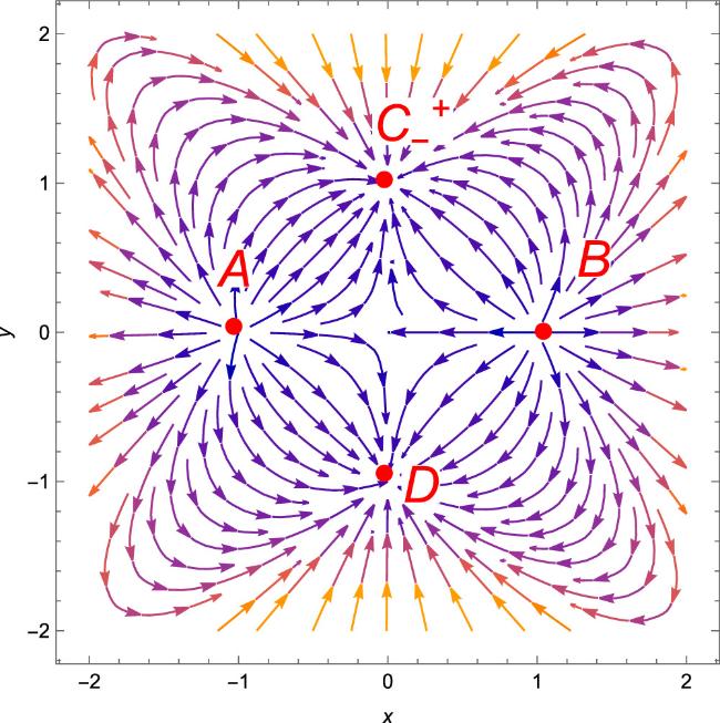
Figure 1. Phase portrait for the system of equations ( |
For the equilibrium points C+ and C−, the eigenvalues are identical. From table 2, at equilibrium points C+ and C−, the eigenvalues are γ1 = − 6 + 3τ2, γ2 = − 3τ2 and γ3 = 0. At τ = 1, the eigenvalues become γ1 = − 3, γ2 = − 3 and γ3 = 0. Since each and every eigenvalue is negative, the equilibrium points C+ and C− are stable. From figure 1, we noticed that all the paths for these two points move towards these points, which confirms their stable behavior. The parameters of density for these two points are: ${{\rm{\Omega }}}_{\phi }=\frac{6({\tau }^{2}-1)}{1+2a}+\frac{{\tau }^{2}}{1+4a}\,{\rm{and}}\,{{\rm{\Omega }}}_{{\rm{d}}{\rm{e}}}=1-\frac{6({\tau }^{2}-1)}{1+2a}-\frac{{\tau }^{2}}{1+4a}$ , which satisfy the condition Ωφ + Ωde = 1 and for a = 2.5, Ωφ = 0 and Ωde = 1 depict the Universe’s dark energy dominated stage. Also, from table 1, the deceleration parameter and EoS parameter for these two points ${C}^{+}\,{\rm{and}}\,{C}^{-}\,{\rm{are}}\,q=-1\,{\rm{and}}\omega =-1$ which demonstrate that the Universe belongs to the accelerated phase. By substituting the values of x, y and z in equation (35 ), we get $\frac{\dot{H}}{{H}^{2}}=0$ . The scale factor for points C+ and C− is expressed by solving this expression as: $a(t)={a}_{0}{{\rm{e}}}^{{b}_{3}t}$ . Here, b3 is the integration constant.
From table 2, at equilibrium point D, the eigenvalues are ${\gamma }_{1}=-3+\frac{3}{2}{\zeta }^{2}$ , ${\gamma }_{2}=0\,{\rm{and}}\,{\gamma }_{3}=-3-\frac{3}{2}{\zeta }^{2}$ . At ζ = 1, the eigenvalues become ${\gamma }_{1}=-\frac{3}{2}$ , ${\gamma }_{2}=0\,{\rm{and}}\,{\gamma }_{3}=-\frac{9}{2}$ . Since each and every eigenvalue is negative, the equilibrium point D is stable. From figure 1, we noticed that all the paths for this point move towards this point, which confirms its stable behavior. The parameters of density for this place are: ${{\rm{\Omega }}}_{\phi }=\frac{6{\zeta }^{2}}{1+2\alpha }\,{\rm{and}}\,{{\rm{\Omega }}}_{{\rm{d}}{\rm{e}}}=1-\frac{6{\tau }^{2}}{1+2\alpha }$ , which satisfy the condition Ωφ + Ωde = 1. Also, from table 1, the deceleration parameter and EoS parameter for the point $D\,{\rm{are}}q=-1\,{\rm{and}}\,\omega =-1$ , demonstrating the Universe’s accelerated phase. For the point D, by using the values of x, y and z in equation (35 ), we get $\frac{\dot{H}}{{H}^{2}}=0$ . The scale factor for point D is expressed by solving this expression as: $a(t)={a}_{0}{{\rm{e}}}^{{b}_{3}t}$ . Here, b3 is the integration constant.
Table 1 indicates that the three equilibrium points C+, C−and D possess a zero eigenvalue, suggesting that these points are non-hyperbolic. For non-hyperbolic equilibrium points, Coley [55] has shown that the dimension of the set of eigenvalues is one, which is equal to the number of vanishing eigenvalues. Consequently, the collection of eigenvalues typically exhibits hyperbolic behavior, indicating that the corresponding equilibrium point is stable but not able to function as a global attractor. In our calculation, there is only one eigenvalue that disappears and the set of eigenvalues has one dimension [56]. In other words, a set of eigenvalues has a dimension equal to the number of vanishing eigenvalues. Consequently, the recent observations are consistent for the equilibrium points (C+, C−and D) and they illustrate the Universe’s accelerated stage.
The energy equations for developing the interacting cosmic models are provided by
$\begin{eqnarray}\begin{array}{l}\dot{{\rho }_{{\rm{d}}{\rm{e}}}}+3H(1+{\omega }_{{\rm{d}}{\rm{e}}}){\rho }_{{\rm{d}}{\rm{e}}}={\mathbb{Q}},\\ \dot{{\rho }_{\phi }}+3H(1+{\omega }_{\phi }){\rho }_{\phi }=-{\mathbb{Q}}.\end{array}\end{eqnarray}$
In this case, ${\mathbb{Q}}$ reflects the interaction between the dark energy and scalar field and denotes the energy density flow through ${\mathbb{Q}}$ . This interaction term can be viewed as a minor adjustment to the evolutionary history of the Universe. When ${\mathbb{Q}}\gt 0$ , energy flows from the scalar field (φ) to the dark energy (ρde). On the other hand, if ${\mathbb{Q}}\lt 0$ , the reverse occurs [57]. It is not feasible to deduce the interaction’s suitable form because the dark energy and scalar field characteristics are still mysterious. This interaction component ${\mathbb{Q}}$ is shaped by the product of the energy density function and the Hubble parameter [58]. Thus, the following categories apply to this interaction: (a) ${\mathbb{Q}}$ =${\mathbb{Q}}(H{\rho }_{{\rm{d}}{\rm{e}}})$ , (b) ${\mathbb{Q}}$ =${\mathbb{Q}}(H{\rho }_{\phi })$ , (c) ${\mathbb{Q}}={\mathbb{Q}}[H({\rho }_{{\rm{d}}{\rm{e}}}+{\rho }_{\phi })]\,{\rm{and}}\,({\rm{d}})$ ${\mathbb{Q}}={\mathbb{Q}}(H{\rho }_{\phi },H{\rho }_{{\rm{d}}{\rm{e}}})$ [59]. For our calculations, we select ${\mathbb{Q}}=\psi H{\rho }_{{\rm{d}}{\rm{e}}}$ , in which $\Psi$ is a tiny, dimensionless, positive-definite constant. Thus, the Klein–Gordon equation (23 ) can be written as follows [60]: 31 ) with the above interaction form as follows: 43 )–(45 ). We evaluate the equilibrium points via the equations’ solution $\frac{{\rm{d}}x}{{\rm{d}}N}=\frac{{\rm{d}}y}{{\rm{d}}N}=\frac{{\rm{d}}z}{{\rm{d}}N}=0$ . We evaluate the eigenvalues from the Jacobian matrix at each equilibrium points to represent the stability criteria of our model. The equilibrium points and the cosmological parameters are displayed in table 3.
$\begin{eqnarray}\mathop{\phi }\limits^{\unicode{x02025}}+3H\dot{\phi }=-\frac{{\mathbb{Q}}}{\dot{\phi }}.\end{eqnarray}$
The set of ordinary differential equations can be generated from the variables in equation ( $\begin{eqnarray}\begin{array}{l}\frac{{\rm{d}}x}{{\rm{d}}N}=-\frac{\psi (1+2a)\epsilon }{2x}\left[1-\frac{6{x}^{2}}{1+2a}-\frac{{y}^{2}}{1+4a}\right]\\ \quad -\frac{3x}{2}(1-{x}^{2}+{y}^{2}+z),\end{array}\end{eqnarray}$
$\begin{eqnarray}\frac{{\rm{d}}y}{{\rm{d}}N}=\frac{3}{2}y(1+{x}^{2}-{y}^{2}-z),\end{eqnarray}$
$\begin{eqnarray}\frac{{\rm{d}}z}{{\rm{d}}N}=3z(1+{x}^{2}-{y}^{2}+z),\end{eqnarray}$
where N = loga. We determine the equilibrium points of the system that is represented by the system of equations (Table 3. Physical behavior of the scale factor at each equilibrium points. |
| Points | Accelerating equation | Scale factor | Phase |
|---|---|---|---|
| A | $\dot{H}=-3{H}^{2}$ | $a(t)={a}_{0}{(3t+{b}_{2})}^{\frac{1}{3}}$ | stiff matter |
| B | $\dot{H}=-3{H}^{2}$ | $a(t)={a}_{0}{(3t+{b}_{2})}^{\frac{1}{3}}$ | stiff matter |
| C+ | $\dot{H}=0$ | $a(t)={a}_{0}{{\rm{e}}}^{{b}_{3}t}$ | de-Sitter |
| C− | $\dot{H}=0$ | $a(t)={a}_{0}{{\rm{e}}}^{{b}_{3}t}$ | de-Sitter |
| D | $\dot{H}=0$ | $a(t)={a}_{0}{{\rm{e}}}^{{b}_{3}t}$ | de-Sitter |
The eigenvalues and the stability behavior are given in table 4.
Table 4. Equilibrium points and the cosmological parameters for the system of equations ( |
| Points | x | y | z | q | ω | Ωde | Ωφ |
|---|---|---|---|---|---|---|---|
| A+ | $\sqrt{\frac{1+2a}{6}}$ | 0 | 0 | 2 | 1 | 0 | 1 |
| A− | $-\sqrt{\frac{1+2a}{6}}$ | 0 | 0 | 2 | 1 | 1 | 0 |
| B | $-\sqrt{\frac{1+2a}{7+26a}}$ | $\sqrt{\frac{6(1+4a)}{7+26a}}$ | 0 | − 1 | − 1 | 1 | 0 |
| C | $\sqrt{\frac{1+2a}{7+26a}}$ | $\sqrt{\frac{6(1+4a)}{7+26a}}$ | 0 | − 1 | − 1 | 1 | 0 |
| D+ | $\sqrt{\frac{2a-11}{6}-\frac{1}{2\psi }}$ | 0 | $\frac{2a-5}{6}-\frac{1}{2\psi }$ | − 1 | − 1 | 1 | 0 |
| D− | $-\sqrt{\frac{2a-11}{6}-\frac{1}{2\psi }}$ | 0 | $\frac{2a-5}{6}-\frac{1}{2\psi }$ | − 1 | − 1 | 1 | 0 |
From table 5, we see that the characteristic values of the equilibrium points A+ and A− are identical and they also represent the same stability nature. From table 5, for the equilibrium points A+ and A−, the eigenvalues are γ1 = − 6$\Psi$ + 3, γ2 = 3 and γ3 = 6. If $\Psi$ > 0.5, then all the eigenvalues γ1, γ2 and γ3 are positive. Since all the eigenvalues are positive, the equilibrium points A+ and A− are unstable. From figure 2, we observe that all paths emerging from points A+ and A− indicate their unstable behavior. Moreover, if $\Psi$ < 0.5, the eigenvalue γ1 is negative and another two eigenvalues γ2 and γ3 are positive. Therefore, the equilibrium points A+ and A− exhibit saddle behavior because they possess both positive and negative eigenvalues. Figure 2 illustrates trajectories converging towards points A+ and A−, as well as diverging from them, confirming the saddle behavior of points A+ and A−. The density parameters for the points A+ and A−: Ωφ = 1 and Ωde = 0 depicts the scalar field dominated Universe or stiff matter. Also, from table 6 deceleration parameter and EoS parameter regarding the points A+ and A− are q = 2 and ω = 1, it demonstrates that the Universe is part of the decelerating phase. When we substitute the critical points A+ and A− into the expression for $\frac{\dot{H}}{{H}^{2}}$ in equation (35 ), we obtain: $\frac{\dot{H}}{{H}^{2}}=-3$ for a = 2.5, which leads to the scale factor $a(t)={a}_{0}{(3t+{b}_{2})}^{\frac{1}{3}}$ . Here, b2 is the integration constant. This result suggests a Universe with stiff matter, as the evolution of the scale factor corresponds to the stiff fluid case (ω = 1), which matches the EoS parameter we derived from our analysis of the critical points.
Table 5. Eigenvalues and their stability criteria for the system of equations ( |
| Points | γ1 | γ2 | γ3 | Criteria |
|---|---|---|---|---|
| A+ | − 6$\Psi$ + 3 | 3 | 6 | unstable at $\psi \gt \frac{1}{2}$ and saddle at $\psi \lt \frac{1}{2}$ |
| A− | − 6$\Psi$ + 3 | 3 | 6 | unstable at $\psi \gt \frac{1}{2}$ and saddle at $\psi \lt \frac{1}{2}$ |
| B | $3\psi -\frac{13}{4}$ | $-\frac{11}{4}$ | 0 | stable at $\Psi$≤1 and saddle at $\Psi$ > 1 |
| C | $3\psi -\frac{13}{4}$ | $-\frac{11}{4}$ | 0 | stable at $\Psi$≤1 and saddle at $\Psi$ > 1 |
| D+ | $\frac{-6{\psi }^{2}-12\psi -3}{2\psi }$ | 0 | $\frac{3}{2\psi }$ | stable at $\Psi$ = − 0.5 |
| D− | $\frac{-6{\psi }^{2}-12\psi -3}{2\psi }$ | 0 | $\frac{3}{2\psi }$ | stable at $\Psi$ = − 0.5 |
Table 6. Physical behavior of the scale factor at each equilibrium points. |
| Points | Accelerating equation | Scale factor | Phase |
|---|---|---|---|
| A+ | $\dot{H}=-3{H}^{2}$ | $a(t)={a}_{0}{(3t+{b}_{2})}^{\frac{1}{3}}$ | stiff matter |
| A− | $\dot{H}=-3{H}^{2}$ | $a(t)={a}_{0}{(3t+{b}_{2})}^{\frac{1}{3}}$ | stiff matter |
| B | $\dot{H}=0$ | $a(t)={a}_{0}{{\rm{e}}}^{{b}_{3}t}$ | de-Sitter |
| C | $\dot{H}=0$ | $a(t)={a}_{0}{{\rm{e}}}^{{b}_{3}t}$ | de-Sitter |
| D+ | $\dot{H}=0$ | $a(t)={a}_{0}{{\rm{e}}}^{{b}_{3}t}$ | de-Sitter |
| D− | $\dot{H}=0$ | $a(t)={a}_{0}{{\rm{e}}}^{{b}_{3}t}$ | de-Sitter |
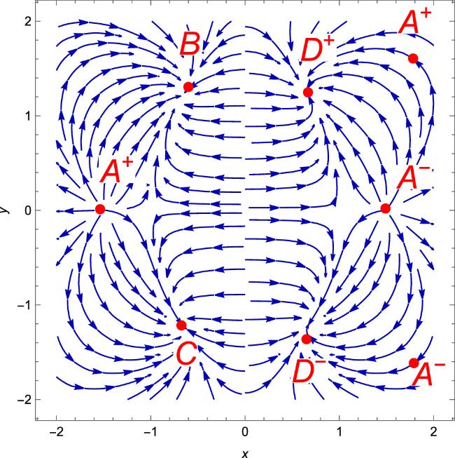
Figure 2. Phase portrait for the system of equations ( |
For equilibrium points B and C, the eigenvalues are identical. From table 5, at equilibrium points B and C, the eigenvalues are ${\gamma }_{1}=3\psi -\frac{13}{4}$ , ${\gamma }_{2}=-\frac{11}{4}$ and γ3 = 0. At $\Psi$≤1 and a = 2.5, the eigenvalues become ${\gamma }_{1}=-\frac{1}{4}$ , ${\gamma }_{2}=-\frac{11}{4}$ and γ3 = 0. Since each and every eigenvalue is negative, the equilibrium points B and C are stable. Observing figure 2, it is evident that all paths converge towards these two points, affirming their stable behavior. Also, for $\Psi$ > 1, the eigenvalue γ1 is negative and another two eigenvalues γ2 and γ3 are positive. Therefore, the equilibrium points B and C exhibit saddle behavior because they possess both positive and negative eigenvalues. The density parameters for points B and C: Ωφ = 0 and Ωde = 1 depict the Universe’s dark energy dominated stage. Also, from table 3, the deceleration parameter and EoS parameter for these two points B and C are q = − 1 and ω = − 1 which demonstrates that the Universe belongs to the accelerated phase. By substituting the values of x, y and z in equation (35 ), we get $\frac{\dot{H}}{{H}^{2}}=0$ for a = 2.5. The scale factor for points B and C is expressed by solving this expression as: $a(t)={a}_{0}{{\rm{e}}}^{{b}_{3}t}$ . Here, b3 is the integration constant.
For the equilibrium points D+ and D−, the eigenvalues are identical. From table 5, at equilibrium points D+ and D−, the eigenvalues are ${\gamma }_{1}=\frac{-6{\psi }^{2}-12\psi -3}{2\psi }$ , γ2 = 0 and ${\gamma }_{3}=\frac{3}{2\psi }$ . At $\Psi$ = − 0.5, the eigenvalues become ${\gamma }_{1}=-\frac{3}{2}$ , γ2 = 0 and γ3 = − 3. Since each and every eigenvalue is negative, the equilibrium points D+ and D− are stable. Observing figure 2, it is evident that all paths converge towards these two points, affirming their stable behavior. The density parameters for points D+ and D−: Ωφ = 0 and Ωde = 1 depict the Universe’s dark energy dominated stage. Also, from table 3, the deceleration parameter and EoS parameter for these two points D+ and D− are q = − 1 and ω = − 1 which demonstrates that the Universe belongs to the accelerated phase. By substituting the values of x, y and z in equation (35 ), we get $\frac{\dot{H}}{{H}^{2}}=0$ for a = 2.5. The scale factor for points D+ and D− is expressed by solving this expression as: $a(t)={a}_{0}{{\rm{e}}}^{{b}_{3}t}$ . Here, b3 is the integration constant.
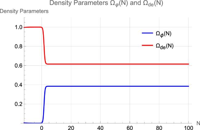
The analysis of the deceleration parameter (q), equation of state parameter (ω) and density parameters Ωde (dark energy) and Ωφ (scalar field) demonstrates that the presented cosmological model in f(R, Tφ) gravity successfully captures the late-time behavior of the Universe. The evolution of the deceleration parameter in figure 3(a) shows that the Universe transitions from a decelerating phase during the matter-dominated era to an accelerating phase as dark energy begins to dominate. This behavior is crucial in explaining the late-time acceleration and the transition is smooth, with q converging to approximately q0 = −0.619, matching observational data. The evolution of the EoS parameter in figure 3(b) shows that dark energy behaves like a cosmological constant at late times, with ω0 ≈ −1, but there may have been small deviations in the past. This supports the idea that the Universe is in a phase of nearly constant dark energy dominance. Figure 4 illustrates the progression of the density parameters. From this figure, we obtain the values of the density parameters as: Ωde = 0.6216 and Ωφ = 0.365 [61, 62]. The condition for a flat universe requires that the total energy density satisfies: Ωde + Ωφ = 1. In our case, Ωde + Ωφ ≈ 0.9866 is quite close to 1 [63]. With Ωde = 0.6216 and Ωφ = 0.365, the Universe is in a phase where dark energy dominates the expansion, but the scalar field still contributes significantly to the overall dynamics and these values suggest that the Universe has not yet reached the final, dark energy-dominated stable point but is on its way. The model is likely transitioning from an earlier scalar field-dominated phase towards a late-time dark energy-dominated phase.
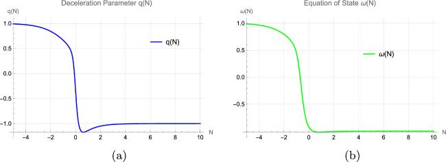
Figure 3. Behavior of deceleration parameter (q) and EoS parameter (ω) with respect to N = loga. |
Figure 4. Behavior of density parameters vs N = loga. |
The deceleration parameter q0 = − 0.619 is consistent with current observations, indicating a Universe in accelerated expansion. Additionally, the equation of state parameter ω0 = −1.00238 aligns closely with the cosmological constant (ω = −1) supporting the dominance of a dark energy component similar to that in ΛCDM model. The density parameters Ωφ = 0.365 and Ωde = 0.6216 reflects the dark energy dominated Universe [56, 64–66].
4. Conclusion
The subject of this study is a flat FRW model of f(R, Tφ) gravity containing a minimally coupled scalar field with self-interacting potential. A specific form, f(R, Tφ) = R + 2f(Tφ), has been recreated to satisfy the Klein–Gordon equation of the scalar field. After reconstruction, the field equations that are equal to the Einstein field equations are f(R, Tφ) =R + 2(aTφ + b). We have analyzed the characteristics of this model by taking the flat potential V0. We perform dynamical system analysis to investigate the stability behavior of this model. We obtain five critical points. The equilibrium points and the physical parameters are evaluated and displayed in table 1. The equilibrium points are A (1, 0, 0), B ( −1, 0, 0), ${C}^{+}\ (\sqrt{{\tau }^{2}-1},\tau ,0)$ , ${C}^{-}\ (-\sqrt{{\tau }^{2}-1},\tau ,0)$ and D (ζ, 0, 1 + ζ2). The equilibrium points A and B are unstable. The density parameters for points A and B are Ωφ = 1 and Ωde = 0 depicts the Universe’s scalar field dominated phase. Also, from table 1, q = 2 and ω = 1, which shows that the Universe belongs to the decelerated phase. The equilibrium points C+ and C− are stable at τ = 1. For the points C+ and C−, Ωφ = 0 and Ωde = 1 depict the Universe’s dark energy dominated phase. Also, from table 1, the deceleration parameter and the EoS parameter for the points C+ and C− are q = − 1 and ω = − 1, which shows that the Universe belongs to the accelerated phase. Again, at ζ = 1, all the eigenvalues for point D are negative, which represents the stable node and Ωφ = 0 and Ωde = 1 depict the Universe’s dark energy dominated phase for this point. q = − 1 and ω = − 1 for point D show the Universe belongs to the accelerated phase. The brief information about the equilibrium points and characteristic values of our model is displayed in tables 1 and 2. The phase space for this model is given in figure 1.
In our work, we assume the form of interaction ${\mathbb{Q}}=\psi H{\rho }_{{\rm{d}}{\rm{e}}}$ . In the interacting model, we evaluate six equilibrium points. The equilibrium points are ${A}^{+}(\sqrt{\frac{1+2a}{6}},0,0)$ , ${A}^{-}\left(-\sqrt{\frac{1+2a}{6}},0,0\right)$ , $B\left(-\sqrt{\frac{1+2a}{7+26a}},\sqrt{\frac{6(1+4a)}{7+26a}},0\right)$ , $C\left(\sqrt{\frac{1+2a}{7+26a}},\sqrt{\frac{6(1+4a)}{7+26a}},0\right)$ , ${D}^{+}\left(\sqrt{\frac{2a-11}{6}-\frac{1}{2\psi }},0,\frac{2a-5}{6}-\frac{1}{2\psi }\right)$ and ${D}^{-}\left(\sqrt{\frac{2a-11}{6}-\frac{1}{2\psi }}\right.$ , $0,\left.\frac{2a-5}{6}-\frac{1}{2\psi }\right)$ . The equilibrium points A+ and A+ are unstable for $\psi \gt \frac{1}{2}$ and saddle for $\psi \lt \frac{1}{2}$ . The density parameters for points A+ and A+ are Ωφ = 1 and Ωde = 0 depict the Universe’s scalar field dominated phase. Also, from table 3, q = 2 and ω = 1 show that the Universe belongs to the decelerated phase. The equilibrium points B and C are stable at $\Psi$ ≤ 1 and saddle at $\Psi$ > 1, a = 2.5. For points B and C, Ωφ = 0 and Ωde = 1 depict the Universe’s dark energy dominated phase. Also, from table 3, the deceleration parameter and the EoS parameter for points B and C are q = − 1 and ω = − 1, which show that the Universe belongs to the accelerated phase. Again, at $\Psi$ = − 0.5, all the eigenvalues for points D+ and D+ are negative representing the stable node and Ωφ = 0 and Ωde = 1 depict the Universe’s dark energy dominated phase for these points. q = − 1 and ω = − 1 for point D+ show the Universe belongs to the accelerated phase. The phase space for this model is given in figure 2. The brief information about the equilibrium points and characteristic values of our model are displayed in tables 3 and 4. Thus, we accomplish that our model is stable and shows the accelerated stage of the Universe.
Acknowledgments
This research is funded by Researchers Supporting Project No. RSPD2025R733, King Saud University, Riyadh, Saudi Arabia.