


1. Introduction
There has been a significant amount of research conducted on the thermodynamics of black holes (BHs) in asymptotically anti-de Sitter (AdS) spacetime. The enchanting phenomenon known as the Hawking–Page transition was first discovered by Hawking and Page. This intriguing event took place at the boundary between a Schwarzschild AdS BH and thermal AdS space, marking a significant phase transition [1, 2]. It is argued that the phase transition of first order experienced by charged AdS BHs is comparable to that experienced by the liquid and gas phase system [3]. Various methods have been developed to calculate entropy corrections, including the utilization of non-perturbative quantum general relativity (GR). Through this approach, researchers have determined the density of microstates for asymptotically flat BHs, leading to logarithmic corrections to the standard Bekenstein entropy-area relationship.
Alternative methodologies have been developed to bring about logarithmic correction terms for various types of BHs, where the microscopic degree of freedom is described through conformal field theory (CFT) [4], loop quantum gravity (LGQ) [5], Hamiltonian partition functions [6], thermodynamic arguments [7], and near horizon symmetries [8]. Emparan et al [9] investigated the behavior of entropy in higher-dimensional BHs and suggested the connection between large and small BHs. Some people have discussed the thermodynamics of Reissner–Nordstrm BHs in higher dimensional AdS spacetime in the presence of higher dimensional entropy [10]. Researchers have looked into how fluctuations affect the entropies of BHs [11]. Schwarzschild BHs’ entropy corrections were discovered by placing it in the center of a sphere with definite radius and setting it to be in equilibrium with its surroundings [12]. The quantum fluctuation's effects on a charged Bañados–Teitelboim–Zanelli (BTZ) BH in asymptotically AdS/dS spacetime have also been examined with the help of massive theory of gravity [13]. In recent work, the effects of fluctuations in temperature for modified Hayward and charged AdS BHs have been examined [14, 15]. The exponential entropies and the thermodynamics of higher-dimensional BHs have been studied, shedding light on the behavior of entropy in various spacetime geometries [16].
There have been some efforts in describing the cosmological constant playing the role as thermodynamic pressure P with thermodynamic volume V as its conjugate variable [17]. The extended phase space has been used in order to analyze thermodynamics and the phase transition of AdS BHs. Kubiznk and Mann [18] evaluated a charged AdS BH's P − V criticality. Additionally, several fascinating AdS BH thermodynamic phenomena have been suggested, such as Joule–Thomson expansion of BHs [19], heat engine efficiency of BHs [20], or transitions between the multiple re-entrant phases [21].
In recent years, many higher-dimensional models have been developed. The well known generalization of Einstein's gravity is Einstein–Gauss–Bonnet (EGB) gravity in which higher-order curvature corrections have been introduced. The leading three terms in Lovelock gravity, namely the cosmological constant, the Einstein–Hilbert action, and the Gauss–Bonnet (GB) term, are all congruent with this theory [22]. The low-energy limit naturally yields GB term [23]. The ghost-free theory (associated field equations consist of metrics second order derivatives) has notable aspects that it possesses the GB term [24]. The BH solutions and their fascinating characteristics in EGB gravity have been investigated in the literature [25, 26].
A singularity with a curvature is present inside of the BH, as one of its most mysterious characteristics. Under some physically reasonable conditions, this curvature singularity is unavoidable in GR due to the renowned singularity theory that Hawking demonstrated. The existence of singularity may be considered as an indication of GR's breaking down. One possible solution could be eliminating the singularity by quantum gravity, whose correct form, however, remains unknown. Bardeen discovered the first instance of such a non singular or regular BH [27], which, as Ayn-Beato and Garcia later pointed out, could be formed due to the gravitational collapse of a particular magnetic monopole within the context of non-linear electrodynamics (NED) [28]. Combining the effects of EGB gravity and NED further enriches the physical properties of higher-dimensional BHs and offers new avenues for exploring their thermodynamics.
Numerous regular BH solutions have been discovered using NED. Some researchers suggested that regular BHs act asymptotically like Reissner–Nordstrm BHs but violate the weak energy condition [29]. Although Bardeen's regular BHs [28] obey the weak energy condition, its asymptotic behavior differs from that of the Reissner–Nordstrm BH. The regular BHs, which satisfy the weak energy condition and behave asymptotically like the Reissner–Nordstrm BH have been studied [30, 31]. Additionally, the Ayn-Beato and Garcia solution was modified to yield the conventional BH solutions [32], in lower dimensional spacetime [33], and in the presence of various dark energy candidates [34]. The other regular BH concepts include radiating Kerr-like regular BHs [35] and rotating regular BHs [36] have been studied and investigated in the literature. The regular BH solutions were discovered also in the EGB gravity [37], the f(T) gravity [38], the f(R) gravity [39], and the quadratic gravity.
In recent years, the study of charged AdS BHs in the framework of EGB gravity and NED has gained significant attention in cosmology and theoretical physics. The interplay between these theoretical constructs has led to intriguing phenomena, such as the emergence of exponential entropy, which holds great promise for understanding the fundamental principles governing the Universe. Thermodynamics and phase structure of charged AdS BHs in the presence of EGB gravity have been studied [40]. The impact of NED on the thermodynamic properties and stability conditions of charged BHs in EGB gravity is also studied [41]. The modification of area law for BHs has been investigated in the higher-order curvature gravity theories, including the EGB term [42]. The study demonstrating the emergence of an exponential correction term to the BH entropy, demonstrates the importance of including higher-order curvature terms in analysis. The physical properties, especially the thermodynamics, of BHs have been discussed for higher-dimensional quartic quasi topological BHs in the framework of non-abelian power Yang–Mills theory [43]. Hyun and Nam [44] investigated thermodynamic properties of charged AdS BHs within the framework of EGB gravity and with the inclusion of NED. In this paper we extend the work of Hyun and Nam [44], to discuss the effect of exponential corrections on thermodynamical behavior for different 5D Ads BHs in extended phase space. Recently, Jawad and his collaborator investigated the thermodynamics and phase transitions of some well known phenomenon in the presence of various BHs entropies [45–52].
There is an extensive body of literature focused on 5D charged AdS BHs, especially in the context of alternative gravity theories and entropy corrections. We have now added comparisons with several significant works that explore similar BH scenarios. Specifically, we have compared our results with the following: our work is based on 5D charged AdS BHs within the framework of EGB gravity, which extends general relativity by including higher-order curvature corrections. Several past studies, such as those by Cai et al [53] and others, have explored the thermodynamics of 5D BHs in this framework. We have included a comparison of our results with their findings, focusing on how the inclusion of exponential entropy corrections in our work modifies the thermodynamic behavior observed in previous studies. For instance, our results show richer phase transition structures and modified critical points due to the exponential corrections, which were not considered in earlier analyses. Other gravity theories, such as Lovelock gravity and f(R) gravity, have also been explored in the context of 5D charged AdS BHs. For instance, Dadhich et al [54] examined BH solutions in Lovelock gravity and found modifications in thermodynamic quantities such as heat capacity and phase transitions. Similarly, studies in f(R) gravity by Hendi et al [55] investigated the thermodynamic stability and critical phenomena in higher-dimensional BHs. We have compared these works to our results, emphasizing that while both Lovelock and f(R) gravity theories introduce higher-order corrections similar to EGB gravity, our use of exponential entropy corrections brings new insights into the stability and phase behavior of BHs, particularly in the presence of nonlinearity in electrodynamics.
The outline of this paper is as follows. In section 2 , we introduce BH solution in EGB gravity. In section 3 , we study thermodynamics of 5D Schwarzschild AdS GB BH (q = 0) using exponential entropy. In section 4 , we discuss thermodynamics of 5D Charged AdS GB BH with Maxwell Electrodynamics (k → 0) using exponential entropy. Finally, we present concluding remarks in section 5 .
2. Black hole in EGB gravity
EGB gravity in 5D coupled to a non-linear electromagnetic field with negative cosmological constant extends Einstein’s general relativity by incorporating higher-dimensional geometry and additional fields [56]. The action describing the system reads 2.1 ). The general solution of this BH is 2.4 ) for f(r+) = 0, where r+ is the BH's horizon radius. It is 2.5 ) and (2.7 ), i.e., 2.11 ), which would have represented a change in volume at the surrounding pressure P, is notable in this context. It is proposed in [63] that the volume of the BH be defined as the thermodynamic variable conjugate to P when the cosmological constant (Λ) is introduced, since $P=-\frac{{\rm{\Lambda }}}{8\pi }$ is a natural candidate for pressure. Equation (2.11 ) should be expressed as follows when the mass is interpreted as the enthalpy, 2.14 ) is naturally regarded as enthalpy and it is given by
$\begin{eqnarray}{ \mathcal S }=\int {{\rm{d}}}^{5}x\sqrt{-g}\left[\displaystyle \frac{1}{16\pi }(-2{\rm{\Lambda }}+R+{\beta \unicode{x00141}}_{\alpha \nu })-\displaystyle \frac{1}{4\pi }\unicode{x00141}(\unicode{x003DD})\right].\end{eqnarray}$
Here, Λ denotes cosmological constant ${\rm{\Lambda }}=-\displaystyle \frac{6}{{\ell }^{2}}$ and GB term Łαν is given as $\begin{eqnarray}{\unicode{x00141}}_{\alpha \nu }={R}^{2}-4{R}_{\gamma \rho }{R}^{\gamma \rho }+{R}_{\gamma \rho \varrho \omega }{R}^{\gamma \rho \varrho \omega },\end{eqnarray}$
where β ≥ 0 is the EGB coupling constant [57], and Ł($\unicode{x003DD}$ ) is the function of invariant $\unicode{x003DD}$ ≡ FabFab/4, where Fab = ∂aAb − ∂bAa is electromagnetic field strength of field Ab [44]. The GB term is a combination of quadratic terms in the curvature tensor that arises in higher-dimensional gravity theories, and it contributes to the equations of motion only when the spacetime dimension is greater than or equal to 5D [58]. The metric for a 5D BH is given in the following expression $\begin{eqnarray}{\rm{d}}{s}^{2}=-f(r){\rm{d}}{t}^{2}+{f}^{-1}(r){\rm{d}}{r}^{2}+{r}^{2}{\rm{d}}{{\rm{\Omega }}}_{3}^{2},\end{eqnarray}$
where t represents time, r is the radial coordinate and ${\rm{d}}{{\rm{\Omega }}}_{3}^{2}$ denotes the line element for unit 3-sphere [59] given as $\begin{eqnarray*}{\rm{d}}{{\rm{\Omega }}}_{3}^{2}={\rm{d}}{\theta }^{2}+{\sin }^{2}\theta {\rm{d}}{\phi }^{2}+{\cos }^{2}\theta {\rm{d}}{\psi }^{2}.\end{eqnarray*}$
The function f(r) depending on the mass of BH, charge, EGB coupling constant, and NED parameters. The general solution of the BH is obtained by solving equations of motion that follow from equation ( $\begin{eqnarray}\begin{array}{l}f(r)=1+\frac{{r}^{2}}{4\beta }\left(1-\sqrt{1-\frac{8\beta }{{\ell }^{2}}+\frac{8\beta }{{r}^{4}}\left(m+\frac{{q}^{2}}{3k}\left({{\rm{e}}}^{-\frac{k}{{r}^{2}}}-1\right)\right)}\right),\end{array}\end{eqnarray}$
where m is the integration constant and also calls the reduced mass of the considered BH. Also, $k\equiv {k}_{o}{\left(\frac{{q}^{2}}{2}\right)}^{\frac{1}{3}}$ , ko is a coupling constant of the NED. This reduced mass is related to the Arnowitt–Deser–Misner (ADM) mass M of the BH solution [60] as $\begin{eqnarray}M=\frac{3{\varpi }_{3}}{16\pi }m.\end{eqnarray}$
Similarly, the total charge Q relates to the reduced charge q as $\begin{eqnarray}q=\frac{4\pi }{{\varpi }_{3}}Q,\end{eqnarray}$
where ϖ3 = 2π2. The relationship between reduced mass m and horizon radius r+ can be determined by solving equation ( $\begin{eqnarray}m={r}_{+}^{2}+2\beta +\frac{{r}_{+}^{4}}{{\ell }^{2}}-\frac{{q}^{2}}{3k}\left({{\rm{e}}}^{-\frac{k}{{r}_{+}^{2}}}-1\right).\end{eqnarray}$
The ADM mass of the BH can be found by using equations ( $\begin{eqnarray}M=\frac{3{\varpi }_{3}}{16\pi }\left({r}_{+}^{2}+2\beta +\frac{{r}_{+}^{4}}{{\ell }^{2}}-\frac{{q}^{2}}{3k}\left({{\rm{e}}}^{-\frac{k}{{r}_{+}^{2}}}-1\right)\right).\end{eqnarray}$
The entropy of the higher-dimensional BH can be derived with help of the Wald formula [61] and is given as $\begin{eqnarray}{S}_{o}=\frac{{\varpi }_{3}{r}_{+}^{3}}{4}\left(1+\frac{12\beta }{{r}_{+}^{2}}\right).\end{eqnarray}$
Here, the second component shows the contribution of the GB term to Einstein's gravity, causing the deviation from the conventional area law [44]. The surface gravity is also used to get the Bekenstein–Hawking temperature of BH [62] as follows $\begin{eqnarray}T=\frac{{f}^{{\prime} }({r}_{+})}{4\pi }.\end{eqnarray}$
The expression for the first law of BH thermodynamics is $\begin{eqnarray}{\rm{d}}M=T{\rm{d}}S+{\rm{\Psi }}{\rm{d}}I+{\rm{\Phi }}{\rm{d}}Q,\end{eqnarray}$
where $T=\frac{\kappa }{2\pi }$ is the Hawking temperature of the BH (with surface gravity κ), $\Psi$ is angular velocity, I is angular momentum, Φ is electrostatic potential difference between the horizon and infinity. It is suggested in [17] that the mass of the BH should actually be examined as enthalpy rather than the usual interpretation of the mass as internal energy in the sense of thermodynamics. The absence of the term PdV in ( $\begin{eqnarray}{\rm{d}}M=T{\rm{d}}S+V{\rm{d}}P+{\rm{\Psi }}{\rm{d}}I+{\rm{\Phi }}{\rm{d}}Q,\end{eqnarray}$
where $V=\left(\right.\frac{\partial M}{\partial P}{\left)\right.}_{S,I,Q}$ is the thermodynamic volume defined in [17]. It has been taken into consideration by a number of authors that Λ should be viewed as a thermodynamic variable that can be changed [64, 65]. The first law of BH thermodynamics in the extended phase space [66] in which the cosmological constant plays pressure’s role as $\begin{eqnarray}P=\frac{3}{4\pi {\ell }^{2}},\end{eqnarray}$
and the ADM mass of the considered BH using equation ( $\begin{eqnarray}{\rm{d}}M=T{\rm{d}}S+{\rm{\Phi }}{\rm{d}}Q+V{\rm{d}}P,\end{eqnarray}$
where S, Q and P are thermodynamic variables for function M(S, Q, P). However, T, Φ and V are variables and conjugate to S, Q and P, respectively.3. Exponential entropy in 5D Schwarzschild AdS GB BH (q = 0)
With vanishing charge q, the metric function of (2.4 ) reduces to 3.4 ). It is observed that the chemical potential Φ is zero in this case because of the absence of charge. Now, the thermodynamic volume V is given by
$\begin{eqnarray}f(r)=1+\frac{{r}^{2}}{4\beta }\left(1-\sqrt{1+\frac{8\beta }{{r}^{4}}m-\frac{8\beta }{{\ell }^{2}}}\right),\end{eqnarray}$
which represents the 5D Schwarzschild AdS GB BH [58]. Here, we discuss the thermodynamic properties of the 5D Schwarzschild AdS GB BH in view of the exponential entropy given in ( $\begin{eqnarray}V={\left(\frac{\partial M}{\partial P}\right)}_{S,Q}=\frac{{\pi }^{2}}{2}{r}_{+}^{4},\end{eqnarray}$
which is just the volume of a sphere with radius r+ in 4D. Understanding the significance of entropy is essential for gaining a comprehensive grasp of the thermodynamic properties of the higher-dimensional BHs and their connections to the broader theories of gravity and thermodynamics [67]. The thermodynamics of higher-dimensional BHs are affected by higher-order corrections to entropy that result from thermal fluctuations. While higher-order corrections are proportional to the inverse of the original entropy, leading order thermal fluctuation as a logarithmic-term in entropy [68]. The investigation of the microscopic roots of entropy is one of the main focus areas in quantum BH physics. Usually, it is expected that a successful quantum theory of a BH should provide an explanation of the Bekenstein–Hawking area law for entropy. Both loop quantum gravity (LQG) and microstate counting in string theory generate Bekenstein–Hawking area law, as well as corrections to it (as an expansion with $\frac{{L}_{p}^{2}}{A}$ , including a logarithmic-term) which has the following general form $\begin{eqnarray}S=\frac{A}{{L}_{p}^{2}}+a\mathrm{ln}\frac{A}{{L}_{p}^{2}}+b\frac{{L}_{p}^{2}}{A}+...+\,\exp \left(-d\frac{A}{{L}_{p}^{2}}\right)+...,\end{eqnarray}$
where a, b, d, etc., are universal constants. The logarithm and subsequent polynomials of $\left(\right.\frac{{L}_{p}^{2}}{A}\left)\right.$ may either not apply to small horizons with areas $O({L}_{p}^{2})$ or apply with modifications [69].In fact, it has been emphasized that if the microstate counting is done in a specific way then for big areas logarithmic corrections do not occur [70]. These terms must be negligible in the tiny-area limit even if they are unavoidable. As an exponentially suppressed correction to the classical result, the leading order Bekenstein–Hawking entropy for the choice of a dimensionless constant $\xi =\frac{\mathrm{ln}2}{2\pi }$ is obtained 3.4 ) represents the exponential entropy correction to the higher-dimensional BHs [71] and is known as exponential entropy. One of the fundamentals of horizon thermodynamics is the Bekenstein–Hawking entropy, while in non-extensive thermodynamics inequivalent entropies might arise. Using non-extensive LQG and relativistic statistical systems [72, 73] to generalize the Boltzmann–Gibbs entropy gives the result [74]3.5 ) represents the exponential correction for non-extensive LQG entropy (or called non-extensive LQG exponential entropy), where n is the entropic index which shows how frequent events have a higher probability than rare ones, $\eta ({\vartheta }_{o})=\frac{\mathrm{ln}2}{\sqrt{3}\pi {\vartheta }_{o}}$ , and ϑo is the Barbero–Immirzi parameter, depending on the gauge group used, which takes the value of $\frac{\mathrm{ln}2}{\pi \sqrt{3}}$ or $\frac{\mathrm{ln}3}{2\pi \sqrt{2}}$ [75]. Using (2.3 ), the temperature of this BH is given by 2.9 ), (3.4 ) and (3.6 ) are used.
$\begin{eqnarray}S=\frac{A{\rm{ln}}2}{8\pi \xi {L}_{p}^{2}}+\exp \left(-\frac{A{\rm{ln}}2}{8\pi \xi {L}_{p}^{2}}\right)={S}_{o}+{{\rm{e}}}^{-{S}_{o}},\end{eqnarray}$
where So is the standard Bekenstein–Hawking entropy. Equation ( $\begin{eqnarray}{S}_{n}=\frac{1}{1-n}\left[\right.{{\rm{e}}}^{(1-n)\eta ({\vartheta }_{o}){S}_{o}}-1\left]\right..\end{eqnarray}$
Equation ( $\begin{eqnarray}T=\frac{3{r}_{+}+8\pi P{r}_{+}^{3}}{6\pi ({r}_{+}^{2}+4\beta )\left(\right.1-{{\rm{e}}}^{-\frac{{\varpi }_{3}{r}_{+}}{4}({r}_{+}^{2}+12\beta )}\left)\right.}.\end{eqnarray}$
Thermal capacity or heat capacity in BH thermodynamics refers to the quantity of heat needed to modify a BH's temperature. Heat capacity at constant pressure is given as $\begin{eqnarray}\begin{array}{rcl}{C}_{P} & = & T{\left(\frac{\partial S}{\partial T}\right)}_{P}=\frac{\partial M}{\partial {r}_{+}}{\left(\frac{\partial T}{\partial {r}_{+}}\right)}^{-1}\\ & = & \left[3{\varpi }_{3}(3{r}_{+}+8\pi P{r}_{+}^{3}){({r}_{+}^{2}+4\beta )}^{2}\right.\\ & & \left.\times \left(\right.1-{{\rm{e}}}^{-\frac{{\varpi }_{3}{r}_{+}}{4}({r}_{+}^{2}+12\beta )}{\left)\right.}^{2}\right]\\ & & \times \left[4\left(3(1+8\pi P{r}_{+}^{2})({r}_{+}^{2}+4\beta )\right.\right.\\ & & \times (1-{{\rm{e}}}^{-\frac{{\varpi }_{3}{r}_{+}}{4}({r}_{+}^{2}+12\beta )})\\ & & -(3{r}_{+}+8\pi P{r}_{+}^{3})[2{r}_{+}(1-{{\rm{e}}}^{-\frac{{\varpi }_{3}{r}_{+}}{4}({r}_{+}^{2}+12\beta )})\\ & & {\left.\left.+\frac{3{\varpi }_{3}}{4}{({r}_{+}^{2}+4\beta )}^{2}{{\rm{e}}}^{-\frac{{\varpi }_{3}{r}_{+}}{4}({r}_{+}^{2}+12\beta )}]\right)\right]}^{-1},\end{array}\end{eqnarray}$
where (The behavior of the heat capacity depending on the horizon radius r+ for various values of pressure P is given in figure 1. The specific heat at constant pressure CP serves as a valuable indicator of the local and global stability of higher-dimensional BHs, especially when considering an exponential corrected entropy model. We can observe that there exist positive, negative and divergence regions in the plot of heat capacity. Basically, the specific heat is related to the response of the black hole to change in its energy. A positive CP implies that an increase in the BH's energy leads to an increase in its entropy. This is crucial for local stability because it indicates that the BH system tends to return to equilibrium after small perturbations. The positivity of CP aligns with the overall increase in entropy and suggests that the corrections contribute to the stability of the BH. A negative CP suggests that an increase in energy leads to a decrease in entropy. This can lead to local instability, as perturbations may grow rather than dissipate. In the context of the exponential corrected entropy model, a negative CP could be associated with specific corrections that impact the stability of the BH, potentially leading to deviations from standard thermodynamic behavior. It is also argued that the first order phase transitions may occur at places where CP vanishes. However, the possibility of second order phase transitions corresponds to the values at which it is infinite. For the specific pressure values, such as $P=\frac{3}{100\pi }$ , no phase transitions occur since the positive nature of the heat capacity CP indicates local stability for the BH. When considering $P=\frac{1}{48\pi }$ , the heat capacity exhibits a positive trend with a higher magnitude compared to $P=\frac{3}{100\pi }$ as the horizon radius r+ increases, suggesting local stability for the BH. However, at $P=\frac{3}{400\pi }$ , the heat capacity experiences divergence at approximately r+ ≈ 1.5 and r+ ≈ 6.4, rendering the BH unstable within the range 1.5 < r+ < 6.4. Nevertheless, the BH achieves thermodynamic stability for r+ < 1.5 and r+ > 6.4, and phase transitions occur between small, intermediate, and large BHs. Additionally, it is noted that the heat capacity remains positive for larger horizon sizes and higher values of P.
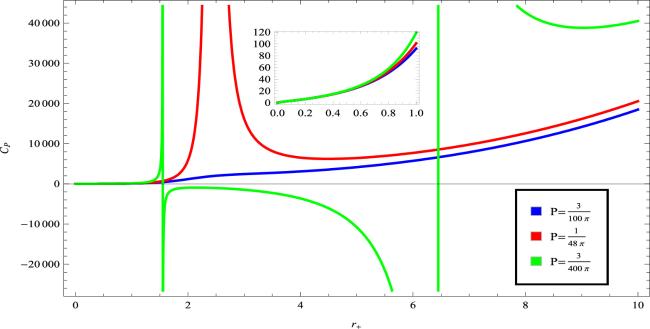
Figure 1. The plot of CP versus r+ of 5D Schwarzschild AdS GB BH for fixed β = 0.5 and different P. |
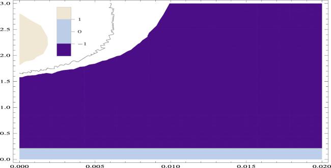
Figure 2 represents the heat capacity and is depicted using a contour plot with a range of values from −1 to 1. The contour regions are color-coded to represent different intervals of CP. The region in the indigo color corresponds to points where the heat capacity takes on the specific value of −1. The indigo color highlights areas where the heat capacity is at its lowest value within the considered range. The slate blue color region represents the interval between −1 and 1 (exclusive). Within this range, the heat capacity varies between −1 and 1. This color coding allows for the identification of points where the heat capacity is moderate and falls within this specified range. The eggshell white color is used to designate points where the heat capacity attains the value of 1. This region stands out as areas where the heat capacity is at its maximum within the considered range. One can see phase transition boundaries where contours changes, providing information about the critical conditions for transitions between different BH phases.
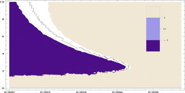
Figure 2. Contour plot of CP versus r+ of 5D Schwarzschild AdS GB BH for fixed β = 0.5 and $P=\frac{3}{400\pi }$ . |
Now by taking into account the free energy, commonly known as Gibbs free energy (GFE) in the grand canonical ensemble, is defined as 3.4 ), (2.13 ), (3.2 ) and (3.6 ), the GFE is given as
$\begin{eqnarray}G=M-TS+PV.\end{eqnarray}$
Hence by using ( $\begin{eqnarray}\begin{array}{rcl}G & = & \frac{{\varpi }_{3}}{16\pi }\left(3{r}_{+}^{2}+6\beta +4\pi P{r}_{+}^{4}\right)\\ & & -\left[\left(3{r}_{+}+8\pi P{r}_{+}^{3}\right)\left(\frac{{\varpi }_{3}{r}_{+}}{4}({r}_{+}^{2}+12\beta \right)\right.\\ & & \left.\left.+{{\rm{e}}}^{-\frac{{\varpi }_{3}{r}_{+}}{4}\left({r}_{+}^{2}+12\beta \right)}\right)\right]\\ & & \times {\left[6\pi ({r}_{+}^{2}+4\beta )\left(1-{{\rm{e}}}^{-\frac{{\varpi }_{3}{r}_{+}}{4}({r}_{+}^{2}+12\beta )}\right)\right]}_{-1}\\ & & +\displaystyle \frac{{\pi }^{2}P{r}_{+}^{4}}{2}.\end{array}\end{eqnarray}$
Figure 3 shows a graphical representation of GFE (G) along with horizon radius (r+) for the fixed value of coupling constant. A positive GFE change implies that a process is non-spontaneous. In the context of BHs, this suggests that the BH is not in a state of thermodynamic stability. Analyzing the thermodynamic implications of positive G provides valuable information about the relative stability of different BH states and the system's tendency to evolve towards more favorable thermodynamic conditions. The GFE is higher for P = 0.02 as compared to P = 0.009, P = 0.003 and P = 0.002. It can be seen that GFE is positive throughout the region. Since GFE tells the global stability of a BH in a grand canonical ensemble. The positive trajectories along the horizon radius for all values of P represent the unstable region.
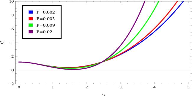
Figure 3. Plot of G versus r+ of 5D Schwarzschild AdS GB BH for fixed β = 0.5 and different P. |
Figure 4 represents the contour graph of G with the contour range [-1,1]. The GFE is positive in both the indigo and the eggshell white color regions. The contour plot of the GFE help us to illustrate the stable and unstable regions for a BH. A BH is stable if it corresponds to a local minimum of GFE at a fixed entropy and other relevant parameters. If the BH is in a region of the contour plot where the GFE is decreasing, it implies stability, whereas an increase in GFE indicates instability.
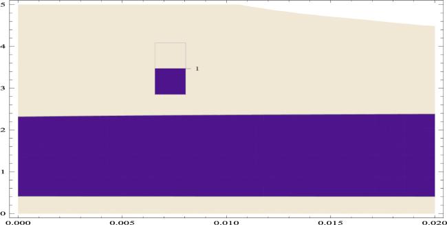
Figure 4. Contour plot of G versus r+ of 5D Schwarzschild AdS GB BH for fixed β = 0.5. |
In the canonical ensemble, the free energy is referred to as the Helmholtz free energy (HFE) when the charge is fixed. The following relation can be used to obtain its expression which is given as 3.8 ) in (3.10 ) leads to the following result 3.9 ) in (3.10 ), the HFE for 5D Schwarzschild AdS GB BH can be obtained as
$\begin{eqnarray}F=G-PV.\end{eqnarray}$
Using ( $\begin{eqnarray}F=M-TS.\end{eqnarray}$
By using ( $\begin{eqnarray}\begin{array}{rcl}F & = & \frac{{\varpi }_{3}}{16\pi }\left(3{r}_{+}^{2}+6\beta +4\pi P{r}_{+}^{4}\right)\\ & & -\left[\left[3{r}_{+}+8\pi P{r}_{+}^{3}\right)\left(\frac{{\varpi }_{3}{r}_{+}}{4}\right.({r}_{+}^{2}+12\beta )\right.\\ & & \left.+{{\rm{e}}}^{-\frac{{\varpi }_{3}{r}_{+}}{4}({r}_{+}^{2}+12\beta )}\right]\\ & & \times \left[6\pi ({r}_{+}^{2}+4\beta )\left(1-{{\rm{e}}}^{-\frac{{\varpi }_{3}{r}_{+}}{4}({r}_{+}^{2}+12\beta )}\right)\right]{}^{-1}.\end{array}\end{eqnarray}$
Figure 5 represents the behavior of HFE against the horizon radius. The Helmholtz free energy provides a thermodynamic potential which determines the stability of a BH in an ensemble with a fixed temperature and entropy. The plot of HFE as a function of the BH horizon radius illustrates the stability conditions for BHs in the context of BH thermodynamics. For P = 0.02, the HFE is positive for r+ < 1.2 and negative for r+ > 1.2. For P = 0.009, the HFE is positive for r+ < 1.4 and negative for r+ > 1.4. For P = 0.003, the HFE is positive for r+ < 7.5 and negative for r+ > 7.5. For P = 0.002, the HFE is positive for r+ < 9.8 and negative for r+ > 9.8. It can be seen that for much smaller values of the horizon radius, the HFE is positive and indicates stability, while it becomes negative for increasing values of r+. It is observed that, the HFE decreases monotonically with P but becomes negative for a larger horizon radius which leads to instability.
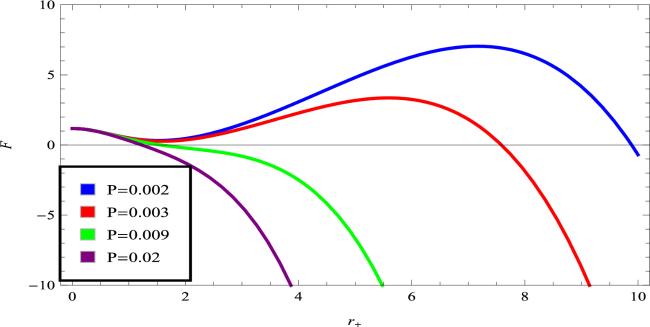
Figure 5. Plot of F versus r+ of 5D Schwarzschild AdS GB BH for fixed β = 0.5 and different P. |
Figure 6 represents the contour graph of F with the contour range [−1,1]. The HFE is negative in the indigo color region for F = −1 and positive in the eggshell white color region for F = 1. The value of F lies between −1 and 0 in the slate blue color region. Similarly, F lies between 0 and 1 in the sky blue color region.
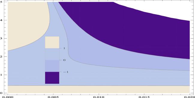
Figure 6. Contour plot of F versus r+ of 5D Schwarzschild AdS GB BH for fixed β = 0.5. |
3.1. Non-extensive LQG exponential entropy
In this case, by considering the second entropy given in (3.5 ), the thermodynamic properties of 5D Schwarzschild AdS GB BH are studied. The results for Φ and V are the same as the previous case, because the change in entropy does not affect volume and chemical potential of the BH.
While the temperature of the BH can be found by using (2.9 ), (3.5 ) and (2.3 ) i.e.,
$\begin{eqnarray}T=\frac{3{r}_{+}+8\pi P{r}_{+}^{3}}{6\pi \eta ({\vartheta }_{o})({r}_{+}^{2}+4\beta ){{\rm{e}}}^{w}}.\end{eqnarray}$
Where $\begin{eqnarray}w=(1-n)\eta ({\vartheta }_{o})\left(\frac{{\varpi }_{3}{r}_{+}}{4}[{r}_{+}^{2}+12\beta ]\right)(Say).\end{eqnarray}$
With the exponential entropy, the heat capacity CP reads
$\begin{eqnarray}\begin{array}{rcl}{C}_{P} & = & \left[3{\varpi }_{3}\eta ({\vartheta }_{o})(3{r}_{+}+8\pi P{r}_{+}^{3}){({r}_{+}^{2}+4\beta )}^{2}{{\rm{e}}}^{2w}\right]\\ & & \times \left[4\left(3(1+8\pi P{r}_{+}^{2})\right.\right.\\ & & \,({r}_{+}^{2}+4\beta ){{\rm{e}}}^{w}-(3{r}_{+}+8\pi P{r}_{+}^{3})\\ & & {\left.\left.\times [2{r}_{+}{{\rm{e}}}^{w}+\mathop{w}\limits^{\unicode{x00301}}({r}_{+}^{2}+4\beta ){{\rm{e}}}^{w}]\right)\right]}^{-1},\end{array}\end{eqnarray}$
where $\begin{eqnarray}\mathop{w}\limits^{\unicode{x00301}}=(1-n)\eta ({\vartheta }_{o})\left(\frac{3{\varpi }_{3}}{4}[{r}_{+}^{2}+4\beta ]\right)(Say).\end{eqnarray}$
In figure 7, we illustrate the influence of non-extensive LQG exponential entropy on the heat capacity of 5D Schwarzschild AdS GB BHs, while maintaining constant values for the coupling constant β, entropic index n, and η. Various values of P are chosen to assess the local stability of the considered BH. For $P=\frac{3}{100\pi }$ and $P=\frac{1}{48\pi }$ , the heat capacity CP remains consistently positive within the range (0 ≤r+ ≤ 10), indicating local stability without any phase transitions. However, for $P=\frac{3}{400\pi }$ , two points of divergence emerge at r+ ≈ 1.5 and r+ ≈ 6.4. Within the range where the horizon radius falls between 1.5 and 6.4, the BH exhibits instability. Conversely, when r+ < 1.5 or r+ > 6.4, the BH achieves thermodynamic stability. Notably, the phase transitions occur between small, intermediate, and large black holes. The graph reveals that the heat capacity is positive for larger horizons and higher values of P, indicating local stability.
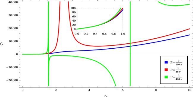
Figure 7. Plot of CP versus r+ of 5D Schwarzschild AdS GB BH for fixed β = 0.5, n = 1.00001, η(ϑo) = 1 and different P. |
Figure 8 represents the heat capacity depicted using a contour plot with a range of values from −1 to 1. The contour regions are color-coded to represent different intervals of CP. This region in the indigo color corresponds to points where the heat capacity takes on the specific value of −1. The indigo color highlights areas where the heat capacity is at its lowest value within the considered range. The slate blue color region represents the interval between −1 and 1 (exclusive). Within this range, the heat capacity varies between −1 and 1. This color coding allows for the identification of points where the heat capacity is moderate and falls within this specified range. The eggshell white color is used to designate points where the heat capacity attains the value of 1. This region stands out as areas where the heat capacity is at its maximum within the considered range. With this entropy, the GFE becomes
$\begin{eqnarray}\begin{array}{rcl}G & = & \displaystyle \frac{{\varpi }_{3}}{16\pi }\left(\right.3{r}_{+}^{2}+6\beta +4\pi P{r}_{+}^{4}\left)\right.\\ & & -\displaystyle \frac{(3{r}_{+}+8\pi P{r}_{+}^{3})({e}^{w}-1)}{6\pi (1-n)\eta ({\vartheta }_{o})({r}_{+}^{2}+4\beta ){{\rm{e}}}^{w}}+\displaystyle \frac{{\pi }^{2}P{r}_{+}^{4}}{2}.\end{array}\end{eqnarray}$
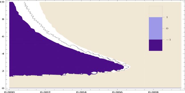
Figure 8. Contour plot of CP versus r+ of 5D Schwarzschild AdS GB BH for fixed β = 0.5, n = 1.00001, η(ϑo) = 1. |
In figure 9, the graph illustrates the correlation between the GFE and the horizon radius, while maintaining constant values for the coupling constant β, entropic index n, and η. A comparison of various values of P, such as 0.02, 0.009, 0.003, and 0.002, reveals that the GFE is notably higher when P = 0.02 in comparison to the other P values. Throughout the entire displayed region on the graph, the GFE consistently maintains a positive value. The GFE serves as an indicator of the overall stability of the BH in the grand canonical ensemble. The positive trajectories observed along the horizon radius for all the specified values of P signify stable regions. This implies that, regardless of the particular P value chosen, the BH remains in a stable state, as indicated by the positive GFE. The graph provides valuable insights into the stability characteristics of the BH under different parameter conditions.
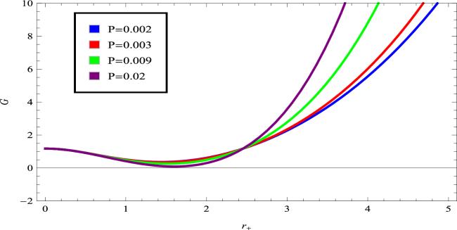
Figure 9. Plot of G versus r+ of 5D Schwarzschild AdS GB BH for fixed β = 0.5, n = 1.00001, η(ϑo) = 1 and different P. |
By inserting (3.5 ) and (3.13 ) into (3.11 ), the HFE F is obtained
$\begin{eqnarray}\begin{array}{rcl}F & = & \displaystyle \frac{{\varpi }_{3}}{16\pi }\left(\right.3{r}_{+}^{2}+6\beta +4\pi P{r}_{+}^{4}\left)\right.\\ & & -\displaystyle \frac{(3{r}_{+}+8\pi P{r}_{+}^{3})({{\rm{e}}}^{w}-1)}{6\pi (1-n)\eta ({\vartheta }_{o})({r}_{+}^{2}+4\beta ){{\rm{e}}}^{w}}.\end{array}\end{eqnarray}$
In figure 10, the behavior of the HFE is depicted in relation to the horizon radius. The purpose is to examine the influence of the second entropy on 5D Schwarzschild AdS GB BHs, assuming a constant coupling constant β and entropic index n. For a value of P = 0.02, the HFE is positive when the horizon radius is r+ < 1.2 and negative when the horizon radius is r+ > 1.3. Similarly, for P = 0.009, the HFE is positive when r+ is below the value 1.4 and negative when r+ > 1.4. This pattern continues for P = 0.003, where the HFE is positive for r+ < 7.2 and negative for r+ > 7.2. Finally, for P = 0.002, the HFE is positive when r+ < 9.1 and negative when r+ > 9.1. It can be observed that for very small values of r+, the HFE is positive, indicating stability. However, as the horizon radius increases, the HFE becomes negative, suggesting instability. Additionally, it is noted that the HFE is higher for P = 0.002 when compared to P = 0.003, P = 0.009, and P = 0.02. Nevertheless, this higher value of HFE for P = 0.002 becomes negative for larger horizon radii, leading to instability. Consequently, in the region between local stability and instability, a second order phase transition occurs.
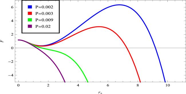
Figure 10. Plot of F versus r+ of 5D Schwarzschild AdS GB BH for fixed β = 0.5, n = 1.00001, η(ϑo) = 1 and different P. |
Figure 11 represents the contour graph of F with the contour range [−1,1]. The HFE is negative in the indigo color region for F = −1 and positive in the eggshell white color region for F = 1. In the slate blue color region, the value of F lies between −1 and 0. Similarly, in the sky blue color region, F lies between 0 and 1.
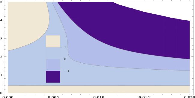
Figure 11. Contour plot of F versus r+ of 5D Schwarzschild AdS GB BH for fixed β = 0.5, n = 1.00001, η(ϑo) = 1. |
4. Exponential entropy in 5D charged AdS GB BH with Maxwell electrodynamics (k → 0)
In (2.4 ), taking the limit k → 0, the metric function reduces to 2.6 ) and (4.3 ) as 3.2 ). The temperature of the BH from (3.4 ) and (4.3 ) is 3.4 ) and (4.5 ) and the relation for the heat capacity given in (3.7 ), we can find CP
$\begin{eqnarray}f(r)=1+\frac{{r}^{2}}{4\beta }\left(1-\sqrt{1-\frac{8\beta }{{\ell }^{2}}+\frac{8\beta m}{{r}^{4}}-\frac{8\beta {q}^{2}}{3{r}^{6}}}\right),\end{eqnarray}$
which describes the EGB gravity charged AdS BH solution. The reduced mass for this BH becomes $\begin{eqnarray}{m}_{2}={r}_{+}^{2}+2\beta +\frac{{r}_{+}^{4}}{{\ell }^{2}}+\frac{{q}^{2}}{3{r}_{+}^{2}}.\end{eqnarray}$
Consequently the ADM mass of the BH reads $\begin{eqnarray}{M}_{2}=\frac{3{\varpi }_{3}}{16\pi }\left({r}_{+}^{2}+2\beta +\frac{{r}_{+}^{4}}{{\ell }^{2}}+\frac{{q}^{2}}{3{r}_{+}^{2}}\right).\end{eqnarray}$
The chemical potential Φ is obtained from ( $\begin{eqnarray}{\rm{\Phi }}={\left(\frac{\partial M}{\partial Q}\right)}_{S,P}=\frac{9Q}{16\pi {r}_{+}^{2}}.\end{eqnarray}$
The thermodynamic volume V of the BH is same as for the 5D Schwarzschild AdS GB BH which is given in ( $\begin{eqnarray}T=\frac{3{r}_{+}+8\pi P{r}_{+}^{3}-\frac{{q}^{2}}{{r}_{+}^{3}}}{6\pi ({r}_{+}^{2}+4\beta )\left(\right.1-{{\rm{e}}}^{-\frac{{\varpi }_{3}{r}_{+}}{4}({r}_{+}^{2}+12\beta )}\left)\right.}\end{eqnarray}$
From ( $\begin{eqnarray}\begin{array}{rcl}{C}_{P} & = & \left[3{\varpi }_{3}(3{r}_{+}+8\pi P{r}_{+}^{3}-\frac{{q}^{2}}{{r}_{+}^{3}}){({r}_{+}^{2}+4\beta )}^{2}\right.\\ & & \left.\times \left(\right.1-{{\rm{e}}}^{-\frac{{\varpi }_{3}{r}_{+}}{4}({r}_{+}^{2}+12\beta )}{\left)\right.}^{2}\right]\\ & & \times \left[4\left(3(1+8\pi P{r}_{+}^{2}+\frac{{q}^{2}}{{r}_{+}^{4}})({r}_{+}^{2}+4\beta )\right.\right.\\ & & \times (1-{{\rm{e}}}^{-\frac{{\varpi }_{3}{r}_{+}}{4}({r}_{+}^{2}+12\beta )})-(3{r}_{+}\\ & & +8\pi P{r}_{+}^{3}-\frac{{q}^{2}}{{r}_{+}^{3}})\left[2{r}_{+}(1-{{\rm{e}}}^{-\frac{{\varpi }_{3}{r}_{+}}{4}({r}_{+}^{2}+12\beta )})\right.\\ & & +\frac{3{\varpi }_{3}}{4}{({r}_{+}^{2}+4\beta )}^{2}\\ & & {\left.\left.\left.\times {{\rm{e}}}^{-\frac{{\varpi }_{3}{r}_{+}}{4}({r}_{+}^{2}+12\beta )}\right]\right)\right]}^{-1}.\end{array}\end{eqnarray}$
The graphical analysis of the heat capacity for the 5D charged AdS BH under Bekenstein–Hawking exponentially corrected entropy at different values of P is represented in figure 12. When $P=\frac{3}{100\pi }$ , the BH is locally stable as CP remains positive in the region along the horizon radius r+ > 0.7 and unstable in the region where r+ > 0.7. So, the second order phase transition takes place. For $P=\frac{1}{48\pi }$ , the small radius region for which r+ < 0.7 has negative capacity and for larger horizon radius r+ > 0.7, the positive trajectory for CP shows that the BH is locally stable. These stable and unstable regions of the BH show the phase transition of the second order. When $P=\frac{3}{400\pi }$ , the BH is unstable in the region of the smaller horizon radius r+ < 0.7 because the capacity is negative in the region and also the curve has two divergent points that occur at r+ ≈ 1.7 and r+ ≈ 6.4. Thus, for the small radius region at which r+ > 0.7 and r+ < 1.7 has a positive heat capacity, therefore the BH is stable in this region. For the intermediate radius which lies between r+ ≈ 1.7 and r+ ≈ 6.4, there is negative heat capacity, therefore the BH is unstable in this region. While the large radius region has positive heat capacity, therefore it is stable and the phase transition takes place between these stable and unstable regions which can be seen in figure 12.
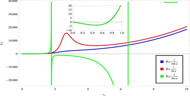
Figure 12. Plot of CP versus r+ of 5D charged AdS GB BH for fixed β = 0.5, q = 0.9 and different p. |
Figure 13 represents the heat capacity with the contour range [ −1,1]. CP is negative in the indigo color region, −1 < CP < 1 in the slate blue color region and positive in the eggshell white color region. One can observe that the stable and unstable regions of contour plot are consistent with the trajectories in the figure 12. The GFE is obtained from (3.4 ), (3.2 ), (4.3 ) and (4.5 ), and put into (3.8 ) as
$\begin{eqnarray}\begin{array}{rcl}G & = & \frac{{\varpi }_{3}}{16\pi }\left(3{r}_{+}^{2}+6\beta +4\pi P{r}^{4}+\frac{{q}^{2}}{{r}_{+}^{2}}\right)\\ & & -\left[(3{r}_{+}+8\pi P{r}_{+}^{3}-\frac{{q}^{2}}{{r}_{+}^{3}})\left(\frac{{\varpi }_{3}{r}_{+}}{4}({r}_{+}^{2}\right.\right.\\ & & \left.\left.+12\beta )+{{\rm{e}}}^{-\frac{{\varpi }_{3}{r}_{+}}{4}({r}_{+}^{2}+12\beta )}\right)\right]\\ & & \times \left[\right.6\pi ({r}_{+}^{2}+4\beta )\left(\right.1-{{\rm{e}}}^{-\frac{{\varpi }_{3}{r}_{+}}{4}({r}_{+}^{2}+12\beta )}\left)\right.{\left]\right.}^{-1}\\ & & +\frac{{\pi }^{2}P{r}_{+}^{4}}{2}.\end{array}\end{eqnarray}$
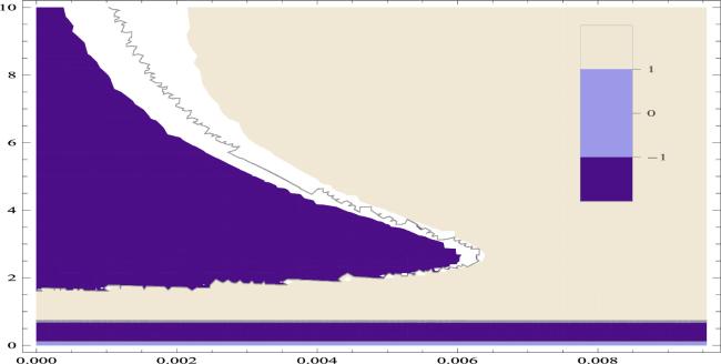
Figure 13. Contour plot of CP versus r+ 5D charged AdS GB BH for fixed β = 0.5, q = 0.9. |
In figure 14, it can be observed that the graph illustrating the relationship between the GFE and the horizon radius for a fixed value of the coupling constant and charge but different values of pressure. The GFE is higher when P = 0.02, compared to the values P = 0.009, P = 0.003, and P = 0.002. It is evident that the GFE remains positive throughout the entire region. Since the GFE provides information about global stability of the BH in the grand canonical ensemble, the positive trajectories along the horizon radius for all these values of P indicate a stable region.

Figure 14. Plot of G versus r+ of 5D charged AdS GB BH for fixed β = 0.5, q = 0.9 and different p. |
The contour graph depicted in figure 15 illustrates the behavior of the function G over a specified domain, with contour lines corresponding to different values of G. The contour range is set between −1 and 1. In the visualization, two distinct regions are highlighted by colors: indigo and eggshell white. The contours within these regions represent specific values of the function G. Notably, the GFE associated with the system is observed to be positive throughout both the indigo and eggshell white regions. This positivity of the GFE in these color-defined areas implies that, within the given parameter space or domain of interest, the system is energetically favorable or has a favorable thermodynamic state. The contour graph serves as a visual representation, aiding in the interpretation of the behavior and trends of the function G in relation to the specified contour range. Equations (3.10 ) and (4.7 ) give the value of the HFE as
$\begin{eqnarray}\begin{array}{rcl}F & = & \frac{{\varpi }_{3}}{16\pi }\left(3{r}_{+}^{2}+6\beta +4\pi P{r}^{4}+\frac{{q}^{2}}{{r}_{+}^{2}}\right)\\ & & -\left[(3{r}_{+}+8\pi P{r}_{+}^{3}-\frac{{q}^{2}}{{r}_{+}^{3}})\left(\frac{{\varpi }_{3}{r}_{+}}{4}({r}_{+}^{2}+12\beta )\right.\right.\\ & & \left.\left.+{{\rm{e}}}^{-\frac{{\varpi }_{3}{r}_{+}}{4}({r}_{+}^{2}+12\beta )}\right)\right]\\ & & \times \left[\right.6\pi ({r}_{+}^{2}+4\beta )\left(\right.1-{{\rm{e}}}^{-\frac{{\varpi }_{3}{r}_{+}}{4}({r}_{+}^{2}+12\beta )}\left)\right.{\left]\right.}^{-1}.\end{array}\end{eqnarray}$
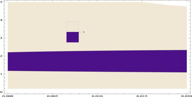
Figure 15. Contour plot of G versus r+ of 5D charged AdS GB BH for fixed β = 0.5, q = 0.9. |
Figure 16 illustrates the variation of the HFE with respect to the horizon radius. For a pressure value of P = 0.02, the HFE is positive when the horizon radius r+ is less than 1.4 and becomes negative for r+ > 1.4. Similarly, at P = 0.009, the HFE is positive for r+ < 1.9 and negative for r+ > 1.9. As the pressure decreases to P = 0.003, the HFE is positive for r+ < 7.5 and negative for r+ > 7.5. Finally, for P = 0.002, the HFE is positive for r+ < 9.8 and negative for r+ > 9.8. An interesting observation is that when the horizon radius is small, the HFE is positive, indicating the stability of the BH. However, as the horizon radius increases, the HFE becomes negative, signaling the instability of the BH. Notably, the HFE is comparatively higher for P = 0.002, than for P = 0.003, P = 0.009, and P = 0.02. Nevertheless, it also undergoes a transition to negativity for the larger horizon radii, indicating instability. This shift in BH trajectories from stability to instability represents a second-order phase transition.
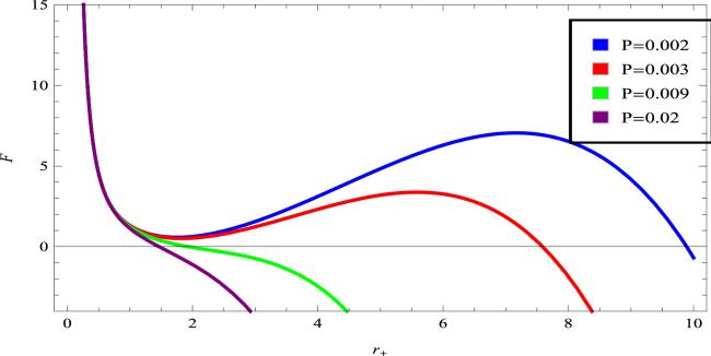
Figure 16. Plot of F versus r+ of 5D charged AdS GB BH for fixed β = 0.5, q = 0.9 and different p. |
When both the charge and entropy are treated as variables, it comes to the grand canonical ensemble. In addition to specific heat and Hawking temperature, the local thermodynamic stability can be guaranteed from the positivity through another criteria which is called the trace of Hessian matrix. The matrix is defined as
$\begin{eqnarray}H=\left[\begin{array}{cc}{H}_{11} & {H}_{12}\\ {H}_{21} & {H}_{22}\\ \end{array}\right],\end{eqnarray}$
where ${H}_{11}=\left(\frac{{\partial }^{2}F}{\partial {T}^{2}}\right),\,{H}_{12}=\left(\frac{{\partial }^{2}F}{\partial T\partial {\rm{\Phi }}}\right),\,{H}_{21}=\left(\frac{{\partial }^{2}F}{\partial {\rm{\Phi }}\partial T}\right),\,{H}_{22}=\left(\frac{{\partial }^{2}F}{\partial {{\rm{\Phi }}}^{2}}\right)$ . It should be noted that some of the eigenvalues of this system are zero (H12H21 = H21H12), so in order to check the stability of the system, the trace of Hessian matrix is used, which is given as $\begin{eqnarray}{\tau }_{H}\equiv {T}_{r}(H)={H}_{11}+{H}_{22}.\end{eqnarray}$
When τH ≥0, the system is locally stable. For such a BH, the trace of Hessian matrix becomes $\begin{eqnarray}{\tau }_{H}=\frac{1}{{X}_{1}}\left(\frac{\mathop{{Y}_{1}}\limits^{\unicode{x00301}}}{{X}_{1}}-\frac{{Y}_{1}\mathop{{X}_{1}}\limits^{\unicode{x00301}}}{{X}_{1}^{2}}\right)+\frac{1}{{Z}_{1}}\left(\frac{\mathop{{Y}_{1}}\limits^{\unicode{x00301}}}{{Z}_{1}}-\frac{{Y}_{1}\mathop{{Z}_{1}}\limits^{\unicode{x00301}}}{{Z}_{1}^{2}}\right),\end{eqnarray}$
where
$\begin{eqnarray*}\begin{array}{rcl}{X}_{1} & = & \frac{\partial T}{\partial {r}_{+}}=-\frac{{r}_{+}\left(3{r}_{+}+8\pi P{r}_{+}^{3}-\frac{{q}^{2}}{{r}_{+}^{3}}\right)}{3\pi \left(1-{{\rm{e}}}^{-{S}_{o}}\right){\left({r}_{+}^{2}+4\beta \right)}^{2}}\\ & & +\frac{\left(1+8\pi P{r}_{+}^{2}+\frac{{q}^{2}}{{r}_{+}^{4}}\right)}{2\pi \left(\right.1-{{\rm{e}}}^{-{S}_{o}}\left)\right.\left(\right.{r}_{+}^{2}+4\beta \left)\right.}-\frac{\mathop{{S}_{o}}\limits^{\unicode{x00301}}\left(3{r}_{+}+8\pi P{r}_{+}^{3}-\frac{{q}^{2}}{{r}_{+}^{3}}\right){{\rm{e}}}^{-{S}_{o}}}{6\pi \left(\right.1-{{\rm{e}}}^{-{S}_{o}}{\left)\right.}^{2}\left(\right.{r}_{+}^{2}+4\beta \left)\right.},\\ \mathop{{X}_{1}}\limits^{\unicode{x00301}} & = & \frac{\partial {X}_{1}}{\partial {r}_{+}},\\ {Y}_{1} & = & \frac{\partial F}{\partial {r}_{+}}=\frac{{\varpi }_{3}(3{r}_{+}+8\pi P{r}_{+}^{3}-\frac{{q}^{2}}{{r}_{+}^{3}})}{8\pi }\\ & & +\frac{{r}_{+}\left(3{r}_{+}+8\pi P{r}_{+}^{3}-\frac{{q}^{2}}{{r}_{+}^{3}}\right)({S}_{o}+{{\rm{e}}}^{-{S}_{o}})}{3\pi \left(\right.1-{{\rm{e}}}^{-{S}_{o}}\left)\right.\left(\right.{r}_{+}^{2}+4\beta {\left)\right.}^{2}}\\ & & -\frac{\left(1+8\pi P{r}_{+}^{2}+\frac{{q}^{2}}{{r}_{+}^{4}}\right)({S}_{o}+{{\rm{e}}}^{-{S}_{o}})}{2\pi \left(\right.1-{{\rm{e}}}^{-{S}_{o}}\left)\right.\left(\right.{r}_{+}^{2}+4\beta \left)\right.}\\ & & +\frac{\mathop{{S}_{o}}\limits^{\unicode{x00301}}\left(3{r}_{+}+8\pi P{r}_{+}^{3}-\frac{{q}^{2}}{{r}_{+}^{3}}\right)({S}_{o}+{{\rm{e}}}^{-{S}_{o}}){e}^{-{S}_{o}}}{6\pi \left(\right.1-{{\rm{e}}}^{-{S}_{o}}{\left)\right.}^{2}\left(\right.{r}_{+}^{2}+4\beta \left)\right.}\\ & & -\frac{\mathop{{S}_{o}}\limits^{\unicode{x00301}}\left(3{r}_{+}+8\pi P{r}_{+}^{3}-\frac{{q}^{2}}{{r}_{+}^{3}}\right)(1-{{\rm{e}}}^{-{S}_{o}})}{6\pi \left(\right.1-{{\rm{e}}}^{-{S}_{o}}\left)\right.\left(\right.{r}_{+}^{2}+4\beta \left)\right.},\\ \mathop{{Y}_{1}}\limits^{\unicode{x00301}} & = & \frac{\partial {Y}_{1}}{\partial {r}_{+}},\\ {Z}_{1} & = & \frac{\partial {\rm{\Phi }}}{\partial {r}_{+}}=-\frac{9Q}{8\pi {r}_{+}^{3}},\\ \mathop{{Z}_{1}}\limits^{\unicode{x00301}} & = & \frac{\partial {X}_{1}}{\partial {r}_{+}}.\end{array}\end{eqnarray*}$
The graph presented in figure 17 depicts the relationship between the trace of the Hessian matrix (τH) and the horizon radius (r+) for a BH under various values of the pressure parameter P. This plot serves as an indicator of the thermodynamic stability of the BH in the grand canonical ensemble. The key observation from the graph is that as the horizon radius (r+) increases, the trace of the Hessian matrix (τH) becomes negative. This negative value of τH is indicative of thermodynamic instability for the BH across the entire region under consideration. In the context of the grand canonical ensemble, the negative values of τH as r+ increases suggest that the BH undergoes an unstable behavior. The trace of the Hessian matrix is often utilized in the study of critical points in thermodynamics, and a negative value implies that small fluctuations or perturbations in the system could lead to further unfavorable changes, indicating instability. Therefore, the overall interpretation of the graph is that, under different values of the pressure parameter P, the BH is thermodynamically unstable in the grand canonical ensemble, and this instability persists as the horizon radius increases throughout the specified region.
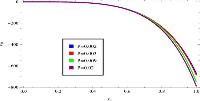
Figure 17. Plot of τH versus r+ of 5D charged AdS GB BH for fixed β = 0.5, q = 0.9 and different p. |
The graph depicted in figure 18 illustrates the trace of the Hessian matrix over a specified range with contours between -1 and 1. The color-coded regions on the graph provide information about the behavior of the trace of the Hessian matrix (τH). In the indigo color region, the contours correspond to negative values of τH. This indicates that within this region, the trace of the Hessian matrix is negative. In the sky blue and eggshell white color regions, the contours correspond to non-negative values of τH. This implies that the trace of the Hessian matrix is either zero or positive within these color regions. The color-coded representation aids in visually identifying the regions where the trace of the Hessian matrix is negative and where it is non-negative. This information is valuable for understanding the thermodynamic characteristics or stability of the system, as the sign of the trace of the Hessian matrix is often associated with the stability properties of a physical system.
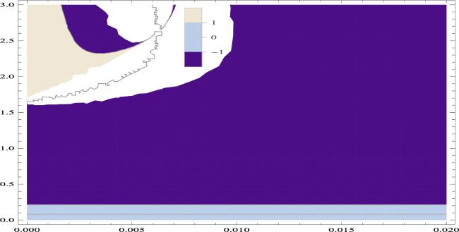
Figure 18. Contour plot of τH versus r+ of 5D charged AdS GB BH for fixed β = 0.5, q = 0.9. |
4.1. Non-extensive LQG exponential entropy
Since the change in entropy does not effect Φ and V by the first law of thermodynamics for higher-dimensional BHs given in (2.14 ). So the values for the BH temperature and heat capacity are given as
$\begin{eqnarray}T=\frac{3{r}_{+}+8\pi P{r}_{+}^{3}-\frac{{q}^{2}}{{r}_{+}^{3}}}{6\pi \eta ({\vartheta }_{o})({r}_{+}^{2}+4\beta ){{\rm{e}}}^{w}},\end{eqnarray}$
$\begin{eqnarray}\begin{array}{rcl}{C}_{P} & = & \left[3{\varpi }_{3}\eta ({\vartheta }_{o})\left(3{r}_{+}+8\pi P{r}_{+}^{3}-\frac{{q}^{2}}{{r}_{+}^{3}}\right)\right.\\ & & \left.\times {({r}_{+}^{2}+4\beta )}^{2}{{\rm{e}}}^{2w}\right]\\ & & \times \left[4\left(3(1+8\pi P{r}_{+}^{2}+\frac{{q}^{2}}{{r}_{+}^{4}})({r}_{+}^{2}+4\beta )\right.\right.\\ & & \times {{\rm{e}}}^{w}-(3{r}_{+}+8\pi P{r}_{+}^{3}\\ & & {\left.\left.-\frac{{q}^{2}}{{r}_{+}^{3}})[2{r}_{+}{e}^{w}+\mathop{w}\limits^{\unicode{x00301}}({r}_{+}^{2}+4\beta ){{\rm{e}}}^{w}]\right)\right]}^{-1},\end{array}\end{eqnarray}$
respectively.The graph in figure 19 illustrates the analysis of heat capacity for a 5D charged AdS BH under fixed values of the coupling constant β, entropic index n, and η, while varying the parameter P. When $P=\frac{3}{100\pi }$ , the BH is locally stable, as the heat capacity CP remains positive in the region where the horizon radius r+ > 0.7. Conversely, in the region where r+ < 0.7, the BH is unstable, indicating a second-order phase transition. For $P=\frac{1}{48\pi }$ , the BH exhibits negative capacity in the region with a small radii (r+ < 0.7). However, it becomes locally stable for larger horizon radii (r+ > 0.7), where the trajectory of CP is positive. The stable and unstable regions imply a second-order phase transition. When $P=\frac{3}{400\pi }$ , the BH is unstable in the region of smaller horizon radii (r+ < 0.7) due to negative capacity. The graph also reveals two divergent points at r+ ≈ 1.7 and r+ ≈ 6.4. In the region with a smaller radii (0.7 < r+ < 1.7), positive heat capacity indicates stability. However, between r+ ≈ 1.7 and r+ ≈ 6.4, negative heat capacity suggests instability. The figure demonstrates that the region of the BH with a very small horizon radius has negative heat capacity, while for a very large horizon radii, it has positive heat capacity, signifying instability and stability, respectively. The phase transition occurs between these stable and unstable regions, as depicted in the figure.
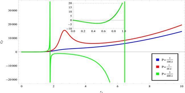
Figure 19. Plot of CP versus r+ of 5D charged AdS GB BH for fixed β = 0.5, q = 0.8, n = 1.00001, η(ϑo) = 1 and different p. |
The graph presented in figure 20 illustrates the behavior of CP with contours within a specified range of [−1,1]. The color-coded regions on the graph provide information about the sign and magnitude of the heat capacity. In the indigo color region, the contours correspond to negative values of CP. This indicates that within this region, the heat capacity is negative. In the slate blue color region, the contours correspond to values of CP between -1 and 1. This suggests that the heat capacity lies within this range in the slate blue region. In the eggshell white color region, the contours correspond to positive values of CP. This indicates that within this region, the heat capacity is positive. The color-coded representation aids in visually identifying the regions where the heat capacity is negative, where it lies between -1 and 1, and where it is positive. Such information is crucial for understanding the thermodynamic properties of the system, as the sign of the heat capacity is often associated with the stability or instability of the system.
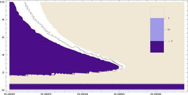
Figure 20. Contour plot of Cp versus r+ of 5D charged AdS GB BH for fixed β = 0.5, q = 0.8, n = 1.00001 and η(ϑo) = 1. |
The GFE is given as
$\begin{eqnarray}\begin{array}{rcl}G & = & \displaystyle \frac{{\varpi }_{3}}{16\pi }\left(3{r}_{+}^{2}+6\beta +4\pi P{r}^{4}+\displaystyle \frac{{q}^{2}}{{r}_{+}^{2}}\right)\\ & & -\displaystyle \frac{\left(3{r}_{+}+8\pi P{r}_{+}^{3}-\displaystyle \frac{{q}^{2}}{{r}_{+}^{3}}\right)\left({{\rm{e}}}^{w}-1\right)}{6\pi (1-n)\eta ({\vartheta }_{o})({r}_{+}^{2}+4\beta ){{\rm{e}}}^{w}}\\ & & +\displaystyle \frac{{\pi }^{2}P{r}_{+}^{4}}{2}.\end{array}\end{eqnarray}$
The graph in figure 21 illustrates the relationship between the GFE and the horizon radius for a specific configuration of the coupling constant β, parameter η, and charge q, with varying values of the pressure parameter P. Upon comparison of different pressure values, it becomes evident that the GFE is higher when P = 0.02 in comparison to the values P = 0.009, P = 0.003, and P = 0.002. This implies that as the pressure increases, the GFE also increases, indicating a higher energy state of the BH system. Notably, throughout the entire region depicted in the graph, the GFE maintains a positive value. This positive value of the GFE signifies a stable region for the BH in this ensemble under all considered values of P. In other words, the BH remains thermodynamically stable across the entire range of horizon radii for the specified parameter values and varying pressures. In conclusion, the graph indicates that, for the given set of parameters, the BH is stable in this ensemble for all values of P, with a higher GFE associated with higher pressure values.
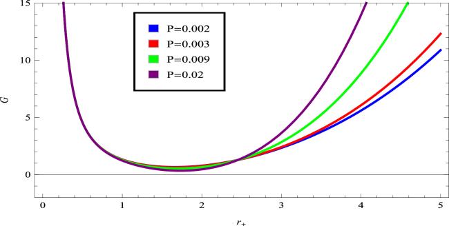
Figure 21. Plot of G versus r+ of 5D charged AdS GB BH for fixed β = 0.5, q = 0.8, n = 1.00001, η(ϑo) = 1 and different p. |
The graph depicted in figure 22 is a contour graph illustrating the behavior of GFE denoted as G, within a specified contour range of [−1,1]. In the graph, two distinct regions are highlighted by different colors: indigo and eggshell white. The contours within these regions represent specific values of the GFE. The key observation is that the GFE is positive throughout both the indigo and the eggshell white color regions. This positivity of the GFE in these color-defined areas indicates that, within the specified parameter space or domain of interest, the system is energetically favorable. In the context of BH thermodynamics, a positive GFE suggests stability. The color-coded representation with contour lines aids in visually identifying the regions where the GFE is positive. This information is valuable for understanding the stability and thermodynamic behavior of the black hole system under consideration. The HFE is given as
$\begin{eqnarray}\begin{array}{rcl}F & = & \frac{{\varpi }_{3}}{16\pi }\left(3{r}_{+}^{2}+6\beta +4\pi P{r}^{4}+\frac{{q}^{2}}{{r}_{+}^{2}}\right)\\ & & -\left[\left(3{r}_{+}+8\pi P{r}_{+}^{3}-\frac{{q}^{2}}{{r}_{+}^{3}}\right)({{\rm{e}}}^{w}-1)\right]\\ & & \times \left[\right.6\pi (1-n)\eta ({\vartheta }_{o})({r}_{+}^{2}+4\beta ){{\rm{e}}}^{w}{\left]\right.}^{-1}.\end{array}\end{eqnarray}$
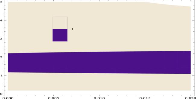
Figure 22. Contour plot of G versus r+ of 5D charged AdS GB BH for fixed β = 0.5, q = 0.8, n = 1.00001 and η(ϑo) = 1. |
Figure 23 illustrates the correlation between the HFE denoted as F and the horizon radius r+ for various values of the pressure parameter P. Specifically, when P = 0.02, the HFE is positive for r+ < 1.4 and negative for r+ > 1.4. For P = 0.009, the HFE is positive for r+ < 1.8 and negative for r+ > 1.8. When P = 0.003, the HFE is positive for r+ < 7.2 and negative for r+ > 7.2. For P = 0.002, the HFE is positive for r+ < 9.1 and negative for r+ > 9.1. In summary, for very small values of the horizon radius, the HFE is positive, indicating the stability of the BH in this region. However, as the horizon radius increases, the HFE becomes negative, signaling the instability of the BH. The graphical representation suggests that the HFE is higher for P = 0.002 compared to P = 0.003, P = 0.009, and P = 0.02, but it becomes negative for larger horizon radii. The observed transitions between the positive and negative values of the HFE for different horizon radii indicate the existence of a second-order phase transition in the regions of local stability and instability.
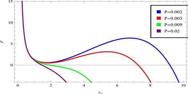
Figure 23. Plot of F versus r+ of 5D charged AdS GB BH for fixed β = 0.5, q = 0.8, n = 1.00001, η(ϑo) = 1 and different p. |
Figure 24 displays a contour graph illustrating the behavior of the HFE denoted as F, with contours within the specified range of [−1,1]. In the graph, different regions are distinguished by varying colors, in the indigo color region, the contours correspond to negative values of F, specifically F = −1. This signifies that within this region, the HFE is negative. In the eggshell white color region, the contours correspond to positive values of F, specifically F = 1. This indicates that within this region, the HFE is positive. In the dark slate blue color region, the contours represent values of F between −1 and 0. In the light slate blue color region, the contours represent values of F between 0 and 1. This color-coded representation helps visually identify the regions where the HFE is negative, where it lies between −1 and 0, where it is between 0 and 1, and where it is positive. Such information is crucial for understanding the stability or instability of the system, as the sign of the HFE is often associated with the thermodynamic behavior of BHs. The results for the trace of the Hessian matrix is given as
$\begin{eqnarray}{\tau }_{H}=\frac{1}{{X}_{2}}\left(\frac{\mathop{{Y}_{2}}\limits^{\unicode{x00301}}}{{X}_{2}}-\frac{{Y}_{2}\mathop{{X}_{2}}\limits^{\unicode{x00301}}}{{X}_{2}^{2}}\right)+\frac{1}{{Z}_{1}}\left(\frac{\mathop{{Y}_{2}}\limits^{\unicode{x00301}}}{{Z}_{1}}-\frac{{Y}_{2}\mathop{{Z}_{1}}\limits^{\unicode{x00301}}}{{Z}_{1}^{2}}\right),\end{eqnarray}$
where $\begin{eqnarray*}\begin{array}{rcl}\mathop{{X}_{2}}\limits^{\unicode{x00301}} & = & \displaystyle \frac{\partial {X}_{2}}{\partial {r}_{+}},\\ {X}_{2} & = & -\displaystyle \frac{{r}_{+}\left(3{r}_{+}+8\pi P{r}_{+}^{3}-\displaystyle \frac{{q}^{2}}{{r}_{+}^{3}}\right){{\rm{e}}}^{-w}}{3\pi \eta ({\vartheta }_{o})\left(\right.{r}_{+}^{2}+4\beta {\left)\right.}^{2}}+\displaystyle \frac{\left(1+8\pi P{r}_{+}^{2}+\displaystyle \frac{{q}^{2}}{{r}_{+}^{4}}\right){{\rm{e}}}^{-w}}{2\pi \eta ({\vartheta }_{o})\left(\right.{r}_{+}^{2}+4\beta \left)\right.}\\ & & -\displaystyle \frac{\mathop{w}\limits^{\unicode{x00301}}\left(3{r}_{+}+8\pi P{r}_{+}^{3}-\displaystyle \frac{{q}^{2}}{{r}_{+}^{3}}\right){{\rm{e}}}^{-w}}{6\pi \eta ({\vartheta }_{o})\left(\right.{r}_{+}^{2}+4\beta \left)\right.},\\ \mathop{{Y}_{2}}\limits^{\unicode{x00301}} & = & \displaystyle \frac{\partial {Y}_{2}}{\partial {r}_{+}},\\ {Y}_{2} & = & \displaystyle \frac{{\varpi }_{3}(3{r}_{+}+8\pi P{r}_{+}^{3}-\displaystyle \frac{{q}^{2}}{{r}_{+}^{3}})}{8\pi }+\displaystyle \frac{{r}_{+}\left(3{r}_{+}+8\pi P{r}_{+}^{3}-\displaystyle \frac{{q}^{2}}{{r}_{+}^{3}}\right)({{\rm{e}}}^{w}-1){{\rm{e}}}^{-w}}{3\pi \eta ({\vartheta }_{o})(1-n)\left(\right.{r}_{+}^{2}+4\beta {\left)\right.}^{2}}\\ & & -\displaystyle \frac{\left(1+8\pi P{r}_{+}^{2}+\displaystyle \frac{{q}^{2}}{{r}_{+}^{4}}\right)({{\rm{e}}}^{w}-1){{\rm{e}}}^{-w}}{2\pi \eta ({\vartheta }_{o})(1-n)\left(\right.{r}_{+}^{2}+4\beta \left)\right.}-\displaystyle \frac{\mathop{w}\limits^{\unicode{x00301}}\left(3{r}_{+}+8\pi P{r}_{+}^{3}-\displaystyle \frac{{q}^{2}}{{r}_{+}^{3}}\right)}{6\pi \eta ({\vartheta }_{o})(1-n)\left(\right.{r}_{+}^{2}+4\beta \left)\right.}\\ & & +\displaystyle \frac{\mathop{w}\limits^{\unicode{x00301}}\left(3{r}_{+}+8\pi P{r}_{+}^{3}-\displaystyle \frac{{q}^{2}}{{r}_{+}^{3}}\right)({{\rm{e}}}^{w}-1){{\rm{e}}}^{-w}}{6\pi \eta ({\vartheta }_{o})(1-n)\left(\right.{r}_{+}^{2}+4\beta \left)\right.}.\end{array}\end{eqnarray*}$
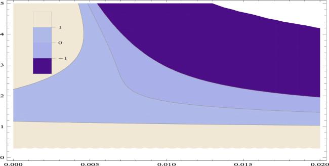
Figure 24. Contour plot of F versus r+ of 5D charged AdS GB BH for fixed β = 0.5, q = 0.8, n = 1.00001 and η(ϑo) = 1. |
Figure 25 illustrates the connection between the trace of the Hessian matrix, denoted as τH (as given in above relation), and the horizon radius for a BH under different values of the pressure parameter P. The plot offers valuable insights into the thermodynamic stability of the BH in the grand canonical ensemble. The key observation from the graph is that the BH is thermodynamically unstable as the horizon radius increases. This inference is drawn from the fact that the trace of the Hessian matrix, τH, is negative (τH < 0) in the plotted region. In the context of thermodynamics, a negative value of τH typically indicates instability. Therefore, as the horizon radius of the BH increases, the system exhibits unstable thermodynamic behavior. The trace of the Hessian matrix is commonly used in the study of critical points and stability properties in thermodynamics. The negative values of τH as the horizon radius increases suggest that the BH undergoes instability in the grand canonical ensemble.
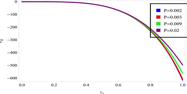
Figure 25. Plot of τH versus r+ of 5D charged AdS GB BH for fixed β = 0.5, q = 0.8, n = 1.00001, η(ϑo) = 1 and different p. |
Figure 26 displays a contour graph representing the trace of the Hessian matrix (τH) with contours within the specified range of [–1,1]. The graph is color-coded to distinguish different ranges of τH. In the indigo color region, the contours correspond to negative values of τH. Specifically, τH is negative in this region. In the sky blue color region, the contours represent values of τH between −1 and 1. The range from −1 < τH < 1 falls within this region. In the eggshell white color region, the contour lines correspond to a specific value of τH = 1. This color-coded representation helps visually identify the regions where the trace of the Hessian matrix is negative, where it lies between −1 and 1, and where it is equal to 1. Such information is crucial for understanding the thermodynamic stability or instability of the BH system, as the sign and magnitude of the trace of the Hessian matrix are often associated with the stability properties in thermodynamics.
Figure 26. Contour plot of τH versus r+ of 5D charged AdS GB BH for fixed β = 0.5, q = 0.8, n = 1.00001 and η(ϑo) = 1. |
5. Concluding remarks
We have discussed a well known category of 5D charged AdS black hole solutions within the framework of Einstein–Gauss–Bonnet gravity coupled to an NED field. The investigation encompasses an exploration of the thermodynamics and phase transitions of these BHs in the extended phase space, employing both exponential entropy and non-extensive LQG exponential entropy. Throughout our analysis, we have meticulously scrutinized various facets of these BHs, examining relationships among parameters such as ADM mass, temperature, volume, chemical potential, heat capacity at constant pressure, GFE, HFE, and the trace of the Hessian matrix. Additionally, we have explored the thermodynamic stability of these BHs within both canonical and grand canonical ensembles, shedding light on their phase transitions. The investigation has allowed us to elucidate how the behavior of BHs aligns with the concept of exponentially corrected entropies, particularly when specific parameters are held constant.
To comprehend the stability and phase transitions of the BH, we generated contour graphs representing specific heat, GFE, HFE and the trace of the Hessian matrix with a range of values from −1 to 1. The color coding allowed the identification of points where the mentioned thermodynamic quantities moderate and fall within a specified range. The eggshell white color is used to designate points where the heat capacity attains the value of 1. This region stands out as areas where the heat capacity is at its maximum within the considered range. We analyzed the phase transition boundaries where contours change, providing information about the critical conditions for transitions between different BH phases. Our analytical and graphical methods have been rigorously combined to provide a robust foundation for comprehending the intricacies of thermodynamics in higher-dimensional BHs within the framework of exponentially corrected entropies. This contribution enriches the ongoing discourse in the field of BH thermodynamics and paves the way for further exploration and research in this captivating area of physics. The potential discovery that different thermodynamic properties of BHs exhibit similar behavior under two distinct exponentially corrected entropies would be a noteworthy and intriguing finding. Such a revelation would necessitate further investigation, holding the promise of advancing our understanding of BH physics, the nature of spacetime, and fundamental principles in physics.
Acknowledgments
The authors extend their appreciation to the Deanship of Research and Graduate Studies at King Khalid University for funding this work through Large Research Project under Grant No. RGP2/539/45.