


1. Introduction
Fluids on curved surfaces exhibit abundant phenomena that are absent in planar systems. Significant studies have been conducted to explore the interplay between geometry, topology, and fluid dynamics in various systems, including active matter [1–3], quantum Hall liquids [4–9], and classical fluids [10–13].
Due to the presence of couplings to curvature, quantum vortices have a fundamental role in determining the properties of superfluids on curved surfaces [14, 15]. In gravity environments, superfluids on curved surfaces tend to settle at the bottom of the surface. However, recent advances in experiments with Bose–Einstein condensates on the International Space Station [16] have given rise to a promising possibility to investigate bubble-trapped superfluids in ultracold atomic bubbles [17]. Intrigued by this experimental progress, the research interest in few-body vortex dynamics on curved surfaces has been revitalized [18–20].
To investigate the dynamics of systems comprised of numerous quantum vortices, a vortex fluid [21, 22] is a suitable model. Prior studies have uncovered novel properties of vortex fluids on planar surfaces. For instance, binary vortex fluids are compressible [22] while chiral vortex fluids are incompressible [21]; Additionally, there exists an odd viscous tensor, and the circulation quantum acts as a non-dissipative coefficient for this odd viscosity; Vortex fluids are closely linked to quantum Hall liquids [23] and fractons [24, 25].
Recently, researchers have begun to explore the effects of curvature and topology on the collective dynamics of quantum vortices. Xiong and Yu have obtained a steady-state solution of a rigid rotation of vortex fluids on a spherical surface [26]. In this paper, we will mainly focus on the perturbation properties of this steady-state solution. We consider the problem in the dynamical regime where the number of point vortices is sufficiently large, and the evolution time is not too long such that non-equilibrium processes induced by stochasticity can be neglected. Our theoretical results demonstrate that despite the background being a steady-state flow of rigid rotation, perturbations imposed on it have their own propagation velocities. Moreover, the propagation velocities of the vortex number density wave and the vortex charge density wave differ. This phenomenon cannot be described by continuous vorticity models [27], as such models only have the vorticity ω that corresponds to the vortex charge density and lack a corresponding quantity for the vortex number density. Additionally, our numerical simulation results match well with the theory in a quantitative manner.
2. Vortex fluids on S2 and rigid rotating steady solutions
2.1. Vortex fluids on a sphere
2.1.1. Point vortex model
Generally, Bose–Einstein condensates (BECs) with interaction are a type of superfluid characterized by a macroscopic wave function $\Psi$ that satisfies the Gross-Pitaevski (G-P) equation [28]. The single valuedness of $\Psi$ requires that vortex excitations in BECs have quantized circulations:
$\begin{eqnarray}\begin{array}{rcl}\psi & = & | \psi | {{\rm{e}}}^{{\rm{i}}\theta },\\ \oint {\rm{d}}\vec{r}\cdot \vec{u} & = & \oint {\rm{d}}\vec{r}\cdot \displaystyle \frac{{\hslash }}{m}{\rm{\nabla }}\theta =\displaystyle \frac{{nh}}{m}.\end{array}\end{eqnarray}$
Here, m is the mass of the atoms, $\vec{u}$ is the velocity field inside the superfluid, n is an integer called winding number (in this article, only ±1 are considered), and h is the Planck constant.In many cases, the distance between vortices in a superfluid is much larger than their core size (the healing length [29]). In these cases, the vortex system can be treated as a system of point vortices, whose vorticity is given by a sum of delta functions
$\begin{eqnarray}\omega \left(\vec{r}\right)={\rm{\nabla }}\times \vec{u}=\displaystyle \sum _{i}\displaystyle \frac{{n}_{i}h}{m}\delta \left(\vec{r}-{\vec{r}}_{i}\right)\equiv \displaystyle \sum _{i}{{\rm{\Gamma }}}_{i}\delta \left(\vec{r}-{\vec{r}}_{i}\right),\end{eqnarray}$
where ni, ${\vec{r}}_{i}$ and Γi are the winding number, location and circulation of the ith point vortex, respectively.In the unit spherical case, according to Kimura [30], the above definition of the vorticity should be modified as follows
$\begin{eqnarray}\begin{array}{rcl}\omega (\theta ,\phi ) & = & \displaystyle \sum _{i}{{\rm{\Gamma }}}_{i}\delta \left(\theta ,\phi ;{\theta }_{i},{\phi }_{i}\right)-\displaystyle \frac{{{\rm{\Gamma }}}_{i}}{4\pi }\\ & = & \displaystyle \sum _{i}\displaystyle \frac{{{\rm{\Gamma }}}_{i}}{\sin \theta }\delta \left(\theta -{\theta }_{i}\right)\delta \left(\phi -{\phi }_{i}\right)-\displaystyle \frac{{{\rm{\Gamma }}}_{i}}{4\pi },\end{array}\end{eqnarray}$
where θ and φ are the polar and azimuthal angles, respectively. However, the counter terms proportional to $-\tfrac{1}{4\pi }$ in the definition of vorticity are unphysical in real superfluids since there is no continuous vorticity in superfluids. The only way out is to ask the total circulation to be equal to 0, i.e. ∑iΓi = 0. In that case, all the counter terms cancel neatly among themselves.2.1.2. Vortex fluids on a sphere
In this article, we only consider two types of point vortices, for which the winding number n = ± 1, namely the positive vortex and negative vortex, or vortex and anti-vortex for short. After coarse graining [22], the system is characterized by the vortex number density and vortex charge density
$\begin{eqnarray}\rho (\theta ,\phi )=\displaystyle \sum _{i}\displaystyle \frac{1}{\sin \theta }\delta (\theta -{\theta }_{i})\delta (\phi -{\phi }_{i}),\end{eqnarray}$
$\begin{eqnarray}\sigma (\theta ,\phi )=\displaystyle \sum _{i}\displaystyle \frac{{n}_{i}}{\sin \theta }\delta (\theta -{\theta }_{i})\delta (\phi -{\phi }_{i}),\end{eqnarray}$
or the positive vortex number density and negative vortex number density $\begin{eqnarray}{\rho }^{+}(\theta ,\phi )=\displaystyle \sum _{i=1}^{{N}_{+}}\displaystyle \frac{1}{\sin \theta }\delta (\theta -{\theta }_{i}^{+})\delta (\phi -{\phi }_{i}^{+}),\end{eqnarray}$
$\begin{eqnarray}{\rho }^{-}(\theta ,\phi )=\displaystyle \sum _{i=1}^{{N}_{-}}\displaystyle \frac{1}{\sin \theta }\delta (\theta -{\theta }_{i}^{-})\delta (\phi -{\phi }_{i}^{-}),\end{eqnarray}$
where $({\theta }_{i}^{+},{\phi }_{i}^{+})$ is the coordinate of the ith positive vortex and $({\theta }_{i}^{-},{\phi }_{i}^{-})$ is the coordinate of the ith negative vortex. Meanwhile, the number of positive vortices N+ must be equal to that of negative vortices N−, to ensure the cancelation of total vorticity. By continuity relation the vortex number current and vortex charge current are induced: $\begin{eqnarray}{J}_{n}^{\mu }=\displaystyle \sum _{i}\displaystyle \frac{1}{\sin \theta }\delta (\theta -{\theta }_{i})\delta (\phi -{\phi }_{i}){v}_{i}^{\mu }\equiv \rho {v}^{\mu },\end{eqnarray}$
$\begin{eqnarray}{J}_{c}^{\mu }=\displaystyle \sum _{i}\displaystyle \frac{{n}_{i}}{\sin \theta }\delta (\theta -{\theta }_{i})\delta (\phi -{\phi }_{i}){v}_{i}^{\mu }\equiv \rho {w}^{\mu },\end{eqnarray}$
where ${v}_{i}^{\mu }$ is the velocity of the ith point vortex and its expression is given by Kimura [30], and the coarse-grained vortex number velocity field vμ and vortex charge velocity field wμ for vortex fluids are defined. The continuity equations read $\begin{eqnarray}{\partial }_{t}\rho +{{\rm{\nabla }}}_{\mu }{J}_{n}^{\mu }=0,\end{eqnarray}$
$\begin{eqnarray}{\partial }_{t}\sigma +{{\rm{\nabla }}}_{\mu }{J}_{c}^{\mu }=0,\end{eqnarray}$
where ∇μ is the covariant derivative on the unit sphere. The Helmholtz equation also holds in this case [26] $\begin{eqnarray}{\partial }_{t}\sigma +{v}^{\mu }{{\rm{\nabla }}}_{\mu }\sigma =0.\end{eqnarray}$
2.2. Rigid rotating steady solution
Xiong and Yu [26] obtained a rigid rotating steady solution for vortex fluids on the unit sphere. We cite it here for later use
$\begin{eqnarray}{\rho }_{0}=N/4\pi ,\end{eqnarray}$
$\begin{eqnarray}{\sigma }_{0}={\rho }_{0}\cos \theta ,\end{eqnarray}$
$\begin{eqnarray}{v}_{0}^{\theta }=0,\end{eqnarray}$
$\begin{eqnarray}{v}_{0}^{\phi }=\pi \gamma {\rho }_{0}-\displaystyle \frac{1}{4}\gamma ,\end{eqnarray}$
where $\gamma =\tfrac{{\hslash }}{m}$ and N is the total number of vortices. Obviously, the system is rotating about the axis like a rigid body.3. Density waves on the sphere
3.1. Theory
In this section, we will add perturbations to the rigid rotating background introduced at the end of the last section. To this purpose we write every physical quantity as a sum of two parts, namely the unperturbed part and the perturbation part10 ), (12 ) also in spherical coordinates17 ), (18 ), (19 ), (20 ) into (21 ) (22 ), (23 ), (24 ), we obtain the linearized relations between the perturbation quantitiesappendix ) leads to the following result
$\begin{eqnarray}u={u}_{0}+\delta u,\end{eqnarray}$
$\begin{eqnarray}v={v}_{0}+\delta v,\end{eqnarray}$
$\begin{eqnarray}\rho ={\rho }_{0}+\delta \rho ,\end{eqnarray}$
$\begin{eqnarray}\sigma ={\sigma }_{0}+\delta \sigma .\end{eqnarray}$
At this point, we invoke the following relation between the velocity field of the vortex fluid and of the superfluid from Xiong and Yu [26] $\begin{eqnarray}{v}^{\theta }={u}^{\theta }-\displaystyle \frac{1}{\sin \theta }\displaystyle \frac{\gamma }{4}\displaystyle \frac{1}{\rho }\displaystyle \frac{\partial \sigma }{\partial \phi },\end{eqnarray}$
$\begin{eqnarray}{v}^{\phi }={u}^{\phi }+\displaystyle \frac{1}{\sin \theta }\displaystyle \frac{\gamma }{4}\displaystyle \frac{1}{\rho }\displaystyle \frac{\partial \sigma }{\partial \theta }.\end{eqnarray}$
For later convenience, we rewrite equations ( $\begin{eqnarray}{\partial }_{t}\rho +\displaystyle \frac{1}{\sin \theta }\displaystyle \frac{\partial }{\partial \theta }[\sin \theta \left(\rho {v}^{\theta }\right)]+\displaystyle \frac{\partial }{\partial \phi }\left(\rho {v}^{\phi }\right)=0,\end{eqnarray}$
$\begin{eqnarray}{\partial }_{t}\sigma +{v}^{\theta }\displaystyle \frac{\partial }{\partial \theta }\sigma +{v}^{\phi }\displaystyle \frac{\partial }{\partial \phi }\sigma =0.\end{eqnarray}$
After substituting equations ( $\begin{eqnarray}\delta {v}^{\phi }=\delta {u}^{\phi }+\displaystyle \frac{1}{\sin \theta }\displaystyle \frac{\gamma }{4}\left(\displaystyle \frac{1}{{\rho }_{0}}\displaystyle \frac{\partial \delta \sigma }{\partial \theta }-\displaystyle \frac{\delta \rho }{{\rho }_{0}^{2}}\displaystyle \frac{\partial {\sigma }_{0}}{\partial \theta }\right),\end{eqnarray}$
$\begin{eqnarray}\delta {v}^{\theta }=\delta {u}^{\theta }-\displaystyle \frac{1}{\sin \theta }\displaystyle \frac{\gamma }{4}\left(\displaystyle \frac{1}{{\rho }_{0}}\displaystyle \frac{\partial \delta \sigma }{\partial \phi }-\displaystyle \frac{\delta \rho }{{\rho }_{0}^{2}}\displaystyle \frac{\partial {\sigma }_{0}}{\partial \phi }\right),\end{eqnarray}$
$\begin{eqnarray}{\partial }_{t}\delta \rho +\displaystyle \frac{1}{\sin \theta }\displaystyle \frac{\partial }{\partial \theta }\left[\sin \theta \left({\rho }_{0}\delta {v}^{\theta }+{v}_{0}^{\theta }\delta \rho \right)\right]+\displaystyle \frac{\partial }{\partial \phi }\left({\rho }_{0}\delta {v}^{\phi }\right.\end{eqnarray}$
$\begin{eqnarray}\left.+\,{v}_{0}^{\phi }\delta \rho \right)=0,\end{eqnarray}$
$\begin{eqnarray}{\partial }_{t}\sigma +{v}_{0}^{\theta }\displaystyle \frac{\partial }{\partial \theta }\delta \sigma +{v}_{0}^{\phi }\displaystyle \frac{\partial }{\partial \phi }\delta \sigma +\delta {v}^{\theta }\displaystyle \frac{\partial }{\partial \theta }{\sigma }_{0}+\delta {v}^{\phi }\displaystyle \frac{\partial }{\partial \phi }{\sigma }_{0}=0.\end{eqnarray}$
Since the spherical harmonics are orthonormal and complete on the sphere, we decompose the perturbation quantities into sums of spherical harmonics $\begin{eqnarray}\delta \rho \left(\theta ,\phi ,t\right)=\displaystyle \sum _{{lm}}{R}_{{lm}}\left(t\right){Y}_{{lm}}\left(\theta ,\phi \right),\end{eqnarray}$
$\begin{eqnarray}\delta \sigma \left(\theta ,\phi ,t\right)=\displaystyle \sum _{l\ne 0,m}{S}_{{lm}}\left(t\right){Y}_{{lm}}\left(\theta ,\phi \right).\end{eqnarray}$
Besides, using spherical harmonics as the expansion basis for the perturbation part has the following advantages: The single-mode spherical harmonic perturbation above the rigid rotating background evolves in time as a traveling wave, while other types of perturbation generally do not have such a simple temporal behavior because of dispersion, which we will shortly see. It is worth mentioning that Shankar et al [2] also used the method of linear perturbation about the steady-state solution to explore the dynamic mode in an article on active matters on curved surfaces, although their work did not involve spherical harmonics. The absence of the Y00 component for δσ is the direct result of the requirement that the total vorticity must be equal to 0. A lengthy calculation (see $\begin{eqnarray}{R}_{{lm}}\left(t\right)={R}_{{lm}}\left(0\right)\exp \left(-\displaystyle \frac{{\rm{i}}{mN}\gamma }{4}t\right),\end{eqnarray}$
$\begin{eqnarray}{S}_{{lm}}\left(t\right)={S}_{{lm}}\left(0\right)\exp \left\{-\displaystyle \frac{{\rm{i}}{mN}\gamma }{4}\left[1-\displaystyle \frac{2}{l\left(l+1\right)}\right]t\right\},\end{eqnarray}$
where N is the total number of point vortices constituting the background. Thus for the single-mode initial distribution $\begin{eqnarray}\delta {\rho }_{{lm}}\left(\theta ,\phi ,t=0\right)={P}_{l}^{m}\left(\cos \theta \right)\left(A\cos m\phi +B\sin m\phi \right),\end{eqnarray}$
$\begin{eqnarray}\delta {\sigma }_{{lm}}\left(\theta ,\phi ,t=0\right)={P}_{l}^{m}\left(\cos \theta \right)\left(C\cos m\phi +D\sin m\phi \right),\end{eqnarray}$
the solution is $\begin{eqnarray}\begin{array}{rcl}\delta {\rho }_{{lm}}\left(\theta ,\phi ,t\right) & = & {P}_{l}^{m}\left(\cos \theta \right)\left[A\cos m\left(\phi -\displaystyle \frac{N\gamma }{4}t\right)\right.\\ & & \left.+B\sin m\left(\phi -\displaystyle \frac{N\gamma }{4}t\right)\right],\end{array}\end{eqnarray}$
$\begin{eqnarray}\begin{array}{l}\delta {\sigma }_{{lm}}\left(\theta ,\phi ,t\right)={P}_{l}^{m}\left(\cos \theta \right)\left\{C\cos m\left\{\phi -\displaystyle \frac{N\gamma }{4}\right.\right.\\ \quad \left.\left.\times \left[1-\displaystyle \frac{2}{l\left(l+1\right)}\right]t\right\}+D\sin m\left\{\phi -\displaystyle \frac{N\gamma }{4}\left[1-\displaystyle \frac{2}{l\left(l+1\right)}\right]t\right\}\right\}.\end{array}\end{eqnarray}$
Obviously, this is a wave solution, and the waves are propagating along the equator of the unit sphere. What’s more, the wave velocities for δρlm and δσlm are different and the latter depends on l generally. In the large N limit, the wave velocity for δρlm agrees with the rotating velocity of the rigid background, while the wave velocity for δσlm does not. Therefore, we have found that there exists dispersion for propagating vortex charge density waves even in dynamical regimes.There is another important result, namely the beat phenomenon. If we start from the following initial condition
$\begin{eqnarray}\delta {\rho }^{+}(\theta ,\phi ,0)={A}_{0}{P}_{l}^{m}(\cos \theta )\cos m\phi ,\end{eqnarray}$
$\begin{eqnarray}\delta {\rho }^{-}(\theta ,\phi ,0)=0,\end{eqnarray}$
where A0 is a small number compared to N/4π, then $\begin{eqnarray}\delta \rho (\theta ,\phi ,0)={A}_{0}{P}_{l}^{m}(\cos \theta )\cos m\phi ,\end{eqnarray}$
$\begin{eqnarray}\delta \sigma (\theta ,\phi ,0)={A}_{0}{P}_{l}^{m}(\cos \theta )\cos m\phi .\end{eqnarray}$
Thus we end up with the following traveling wave solution for δρ and δσ $\begin{eqnarray}\delta \rho (\theta ,\phi ,t)={A}_{0}{P}_{l}^{m}(\cos \theta )\cos m\left(\phi -\displaystyle \frac{N\gamma }{4}t\right),\end{eqnarray}$
$\begin{eqnarray}\begin{array}{rcl}\delta \sigma (\theta ,\phi ,t) & = & {A}_{0}{P}_{l}^{m}(\cos \theta )\cos m\\ & & \times \left\{\phi -\displaystyle \frac{N\gamma }{4}\left[1-\displaystyle \frac{2}{l\left(l+1\right)}\right]t\right\}.\end{array}\end{eqnarray}$
Therefore we find $\begin{eqnarray}\begin{array}{rcl}\delta {\rho }^{+} & = & \displaystyle \frac{1}{2}(\delta \rho +\delta \sigma )={A}_{0}{P}_{l}^{m}(\cos \theta )\\ & & \times \,\cos \left[\displaystyle \frac{{mN}\gamma }{4l(l+1)}t\right]\cos m\left\{\phi -\displaystyle \frac{N\gamma }{4}\left[1-\displaystyle \frac{1}{l(l+1)}\right]t\right\},\end{array}\end{eqnarray}$
$\begin{eqnarray}\begin{array}{rcl}\delta {\rho }^{-} & = & \displaystyle \frac{1}{2}(\delta \rho -\delta \sigma )={A}_{0}{P}_{l}^{m}(\cos \theta )\sin \left[\displaystyle \frac{{mN}\gamma }{4l(l+1)}t\right]\\ & & \times \,\sin m\left\{\phi -\displaystyle \frac{N\gamma }{4}\left[1-\displaystyle \frac{1}{l(l+1)}\right]t\right\}.\end{array}\end{eqnarray}$
The above equations clearly show that the amplitudes of the density waves of vortex and anti-vortex themselves oscillate with a frequency of $\tfrac{{mN}\gamma }{4l(l+1)}$ separately, and they differ from each other by a phase difference of π/2. This is indeed a beat phenomenon.3.2. Numerical results
To check our theory, we use numerical methods to simulate the dynamical evolution of point vortex systems on the unit sphere based on the canonical equations [30]. Specifically, the fourth-order Runge-Kutta method is employed to solve the following equations for N vortices
$\begin{eqnarray}\displaystyle \frac{{\rm{d}}{\theta }_{m}}{{\rm{d}}t}=-\displaystyle \frac{1}{4\pi }\displaystyle \sum _{j=1(j\ne m)}^{N}{{\rm{\Gamma }}}_{j}\displaystyle \frac{\sin {\theta }_{j}\sin ({\phi }_{m}-{\phi }_{j})}{1-\cos {\rho }_{{jm}}},\end{eqnarray}$
$\begin{eqnarray}\begin{array}{l}\sin {\theta }_{m}\displaystyle \frac{{\rm{d}}{\phi }_{m}}{{\rm{d}}t}=-\displaystyle \frac{1}{4\pi }\displaystyle \sum _{j=1(j\ne m)}^{N}{{\rm{\Gamma }}}_{j}\\ \quad \times \displaystyle \frac{\cos {\theta }_{j}\sin {\theta }_{j}\cos ({\phi }_{m}-{\phi }_{j})-\sin {\theta }_{m}\cos {\theta }_{j}}{1-\cos {\rho }_{{jm}}},\end{array}\end{eqnarray}$
where Γj = h/m for positive vortices and Γj = − h/m for negative ones and ρjm is the spherical distance between the jth and mth vortices $\begin{eqnarray}\cos {\rho }_{{jm}}=\cos {\theta }_{j}\cos {\theta }_{m}+\sin {\theta }_{j}\sin {\theta }_{m}\cos ({\phi }_{j}-{\phi }_{m}).\end{eqnarray}$
Figure 1 shows the propagation of the vortex number density waves and vortex charge density waves. To obtain a satisfying collective behavior, the total number of vortices should not be too small, since our theory works best in the dynamical regime. When N is relatively small, the stochasticity will play an important role and we should develop a kinetic theory [31]. Meanwhile, to the rigid rotating background, we have to add perturbations, whose stochastic fluctuations also should not be too significant. Through several trials, we found that N = 80000 is a decent choice. We have chosen $\delta \rho =\delta \sigma \propto {\sin }^{2}\theta \cos 2\phi $ (proportional to Y22 + Y2,−2) and $\delta \rho =\delta \sigma \propto {\sin }^{3}\theta \cos 3\phi $ (proportional to Y33 + Y3,−3) instead of $\delta \rho =\delta \sigma \propto \sin \theta \cos \phi $ (proportional to Y11 + Y1,−1) as our examples for the following reasons. When θ → π, $\sin \theta \cos \phi \sim (\pi -\theta )$ . If we have chosen $\delta \rho =\delta \sigma \propto \sin \theta \cos \phi $ , then $\delta {\rho }_{+}\equiv \tfrac{1}{2}(\delta \rho +\delta \sigma )\,\propto \sin \theta \cos \phi \sim (\pi -\theta )$ . Remembering that for our background ${\sigma }_{0}={\rho }_{0}\cos \theta $ , therefore the unperturbed density of positive vortices ${\rho }_{0}^{+}=\tfrac{1}{2}{\rho }_{0}(1+\cos \theta )\sim {\left(\pi -\theta \right)}^{2}$ , which can be much smaller than (π − θ). Thus in some areas δρ+ is even greater than ${\rho }_{0}^{+}$ , which will make the perturbation theory invalid. What is even worse is that ρ0 + δρ < 0 in certain areas, which is absolutely not allowed. Figures 1(a) (b) show the propagation of the vortex number density wave and vortex charge density wave, respectively, with the initial perturbation (at t = t0) sampled according to the distribution $\delta \rho =\delta \sigma \propto {\sin }^{2}\theta \cos 2\phi $ which is the real part of Y22(θ, φ) up to a coefficient. Similarly, figures 1(c) (d) are according to the distribution $\delta \rho =\delta \sigma \propto {\sin }^{3}\theta \cos 3\phi $ which is the real part of Y33(θ, φ) up to a coefficient. t0 through t5 are six evenly-spaced time points. The φ axis is evenly partitioned into 40 intervals and the vortex number and vortex charge within each interval are counted at t = t0, resulting in the blue-colored histograms. The coordinates of positive and negative vortices at t1, t2, t3, t4 and t5 are calculated according to the canonical equations for point vortex systems on the unit sphere given the aforementioned initial perturbations. After the above procedure, sinusoidal curve fittings are used, resulting in the six colored curves in each subfigure. The theory and numerical results match very well. Through the root-finding algorithm, the displacements Δφs from t0 to t5 are found to be 0.398, 0.269, 0.405 and 0.318 for figures 1(a), (b), (c) and (d), respectively. The theoretical predictions are 2/5, 4/15, 2/5 and 1/3, respectively.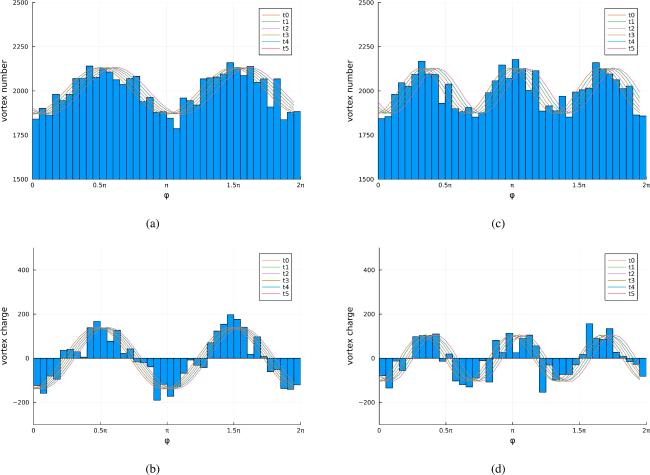
Figure 1. Propagating vortex density waves. |
Figures 2(a)–(e) show the propagation of the density wave of positive vortices with the initial perturbation(at t = t0) sampled according to the distribution $\delta {\rho }^{+}\propto {\sin }^{2}\theta \cos 2\phi $ and δρ− = 0. Similarly, figures 2(f)–(j) show the propagation of the density wave of negative vortices in the same process. The total number of vortices N = 30000, with the numbers of positive and negative vortices being equal. t0 through t4 are five evenly-spaced time points. The φ axis is evenly partitioned into 40 intervals and the positive and negative vortex numbers within each interval are counted at t = t0 s. The coordinates of positive vortices and negative vortices at t1, t2, t3 and t4 are calculated according to the canonical equations for point vortex systems on the unit sphere given the aforementioned initial perturbations. Through the above procedure, 10 histograms are produced and then sinusoidal curve fittings are used, resulting in 10 colored curves. We have carefully chosen t1 such that t1 − t0 is one-eighth of the oscillation period of the amplitudes obtained from equations (44 ), (45 ) so that we expect the amplitude of the positive vortex density wave to reduce to 0 at t2. The theory and numerical results match very well. δρ+ and δρ− go to 0 at t2 and t4, respectively.

Figure 2. Propagating vortex density waves with beat phenomenon. |
4. Conclusions
In this paper, we have investigated the behavior of the perturbations above the axisymmetric rigid rotating state. It is found that the perturbations propagate generally. The propagation velocities for single-mode vortex number density waves are constantly Nγ/4. However, the propagation velocities for single-mode vortex charge density waves depend on the degree of the spherical harmonics l. Thus a general wavelet of perturbation will disperse while propagating. This is a bit counterintuitive since one may naively anticipate that the rigid rotating background will drive everything attached to it to move with the same constant speed as itself.
It is worth noting that we have obtained the velocities for vortex number density waves. If we consider the continuous vortex rather than the point vortex system on S2, then it’s nonsense to talk about the vortex number density waves, since in that case we only have one density, namely the vortex charge density σ or vorticity ω to describe our system. Therefore, the motion of a vortex fluid is different from the motion of the classical vortex of an ideal fluid. The former is a collective description of a large number of point vortices based on the binary point vortex model. It is an emergent phenomenon after taking the positive and negative point vortices as elementary constituents, so it contains more physics than the classical vortex. Our study also provides an example of the interaction between topological defects and curvature, which can be seen when we insert the radius R of the sphere in equations (36 ), (37 ) according to dimensional requirement, and is expected to be useful for investigating rich phenomena involving a large number of quantum vortices [32–34] in bubble-trapped Bose–Einstein condensates [35, 36].
Meanwhile, we find that the amplitudes of the positive and negative vortex density waves oscillate themselves. This phenomenon is a mathematical consequence of the fact that the propagation velocity of the vortex number density wave is different from that of the vortex charge density wave.
Acknowledgments
This work was supported by the Scientific research projects of Hunan Provincial Department of Education (Grant Nos. 22A0477 and 20B273). We also acknowledge L Dai for useful discussions.
Author contributions
YX: Conceptualization, Methodology, Formal Analysis, Writing-Original Draft ZZ: Funding Acquisition, Validation LL: Software, Writing-Review and Editing.
Appendix
We used equations (32 ) and (33 ) in the main text without proving them. Here we provide the derivation. From [30] we know that
$\begin{eqnarray}{u}^{\phi }=-\displaystyle \frac{1}{\sin \theta }\displaystyle \frac{\partial \psi }{\partial \theta },\end{eqnarray}$
$\begin{eqnarray}{u}^{\theta }=\displaystyle \frac{1}{\sin \theta }\displaystyle \frac{\partial \psi }{\partial \phi },\end{eqnarray}$
$\begin{eqnarray}{\rm{\Delta }}\psi =-\omega ,\end{eqnarray}$
where $\Psi$ is the stream function and Δ is the Laplace-Beltrami operator on unit spheres $\begin{eqnarray}{\rm{\Delta }}=\displaystyle \frac{1}{\sin \theta }{\partial }_{\theta }(\sin \theta {\partial }_{\theta })+\displaystyle \frac{1}{{\sin }^{2}\theta }{\partial }_{\phi }^{2}.\end{eqnarray}$
Thus once we know the vorticity ω or charge density σ, by solving the Poisson equation we can obtain the stream function $\Psi$ and the superfluid velocity field u. First, we need to find the Green function for S2 which satisfies the following equation [30],A5 ) Therefore25 ) and (26 ) and we obtain28 ) and (29 ) and obtain32 ) and (33 ).
$\begin{eqnarray}-{\rm{\Delta }}G\left(\theta ,\phi ,\theta ^{\prime} ,\phi ^{\prime} \right)=\displaystyle \frac{1}{\sin \theta }\delta \left(\theta -\theta ^{\prime} \right)\delta \left(\phi -\phi ^{\prime} \right)-\displaystyle \frac{1}{4\pi }.\end{eqnarray}$
Without loss of generality, we assume $\begin{eqnarray}G\left(\theta ,\phi ,\theta ^{\prime} ,\phi ^{\prime} \right)=\displaystyle \sum _{{lm}}{C}_{{lm}}\left(\theta ^{\prime} ,\phi ^{\prime} \right){Y}_{{lm}}\left(\theta ,\phi \right),\end{eqnarray}$
and substitute it into equation ( $\begin{eqnarray}\begin{array}{rcl} & & \displaystyle \sum _{{lm}}l\left(l+1\right){C}_{{lm}}\left(\theta ^{\prime} ,\phi ^{\prime} \right){Y}_{{lm}}\left(\theta ,\phi \right)\\ & = & \displaystyle \frac{1}{\sin \theta }\delta \left(\theta -\theta ^{\prime} \right)\delta \left(\phi -\phi ^{\prime} \right)-\displaystyle \frac{1}{4\pi }\\ & & \times \,k\left(k+1\right){C}_{{kn}}\left(\theta ^{\prime} ,\phi ^{\prime} \right)={Y}_{{kn}}^{* }\left(\theta ^{\prime} ,\phi ^{\prime} \right)\\ & & -\displaystyle \frac{1}{4\pi }{\displaystyle \int }_{0}^{2\pi }{\rm{d}}\phi {\displaystyle \int }_{0}^{\pi }{\rm{d}}\theta \sin \theta {Y}_{{kn}}^{* }\left(\theta ,\phi \right)\\ & & \times \,k\left(k+1\right){C}_{{kn}}\left(\theta ^{\prime} ,\phi ^{\prime} \right)={Y}_{{kn}}^{* }\left(\theta ^{\prime} ,\phi ^{\prime} \right)\\ & & \,-\displaystyle \frac{1}{\sqrt{4\pi }}{\delta }_{k0}{\delta }_{n0}.\end{array}\end{eqnarray}$
• When k ≠ 0,
$\begin{eqnarray}\begin{array}{rcl}k\left(k+1\right){C}_{{kn}}\left(\theta ^{\prime} ,\phi ^{\prime} \right) & = & {Y}_{{kn}}^{* }\left(\theta ^{\prime} ,\phi ^{\prime} \right)\\ {C}_{{kn}}\left(\theta ^{\prime} ,\phi ^{\prime} \right) & = & \displaystyle \frac{1}{k\left(k+1\right)}{Y}_{{kn}}^{* }\left(\theta ^{\prime} ,\phi ^{\prime} \right).\end{array}\end{eqnarray}$
• When k = 0,
$\begin{eqnarray}0=\displaystyle \frac{1}{\sqrt{4\pi }}-\displaystyle \frac{1}{\sqrt{4\pi }}.\end{eqnarray}$
Thus C00 can be any constant and we can set it to be 0. $\begin{eqnarray}G\left(\theta ,\phi ,\theta ^{\prime} ,\phi ^{\prime} \right)=\displaystyle \sum _{l\ne 0,m}\displaystyle \frac{1}{l\left(l+1\right)}{Y}_{{lm}}^{* }\left(\theta ^{\prime} ,\phi ^{\prime} \right){Y}_{{lm}}\left(\theta ,\phi \right).\end{eqnarray}$
With the above Green function, we immediately have $\begin{eqnarray}\begin{array}{rcl}\delta \psi & = & 2\pi \gamma \displaystyle \int {\rm{d}}\theta ^{\prime} {\rm{d}}\phi ^{\prime} \sin \theta ^{\prime} \delta \sigma \left(\theta ^{\prime} ,\phi ^{\prime} \right)\displaystyle \sum _{l\ne 0,m}\displaystyle \frac{1}{l\left(l+1\right)}\\ & & \times {Y}_{{lm}}^{* }\left(\theta ^{\prime} ,\phi ^{\prime} \right){Y}_{{lm}}\left(\theta ,\phi \right)\\ & = & \displaystyle \sum _{l\ne 0,m}\displaystyle \frac{2\pi \gamma }{l\left(l+1\right)}{S}_{{lm}}{Y}_{{lm}}.\end{array}\end{eqnarray}$
Substitute the above solution for δ$\Psi$ into equations ( $\begin{eqnarray}\begin{array}{rcl}\delta {v}^{\phi } & = & -\displaystyle \frac{1}{\sin \theta }\displaystyle \frac{\partial \delta \psi }{\partial \theta }+\displaystyle \frac{1}{\sin \theta }\displaystyle \frac{\gamma }{4}\left(\displaystyle \frac{1}{{\rho }_{0}}\displaystyle \frac{\partial \delta \sigma }{\partial \theta }-\displaystyle \frac{\delta \rho }{{\rho }_{0}^{2}}\displaystyle \frac{\partial {\sigma }_{0}}{\partial \theta }\right)\\ & = & -\displaystyle \sum _{l\ne 0,m}\displaystyle \frac{2\pi \gamma }{l\left(l+1\right)\sin \theta }{S}_{{lm}}\displaystyle \frac{\partial }{\partial \theta }{Y}_{{lm}}+\displaystyle \frac{\gamma }{4{\rho }_{0}\sin \theta }\\ & & \times \displaystyle \sum _{l\ne 0,m}{S}_{{lm}}\displaystyle \frac{\partial }{\partial \theta }{Y}_{{lm}}+\displaystyle \frac{\gamma }{4{\rho }_{0}}\displaystyle \sum _{{lm}}{R}_{{lm}}{Y}_{{lm}}\\ & = & \displaystyle \sum _{l\ne 0,m}\displaystyle \frac{-\tfrac{2}{l\left(l+1\right)}N+1}{4{\rho }_{0}\sin \theta }\gamma {S}_{{lm}}\displaystyle \frac{\partial }{\partial \theta }{Y}_{{lm}}+\displaystyle \frac{\gamma }{4{\rho }_{0}}\displaystyle \sum _{{lm}}{R}_{{lm}}{Y}_{{lm}}\end{array}\end{eqnarray}$
and $\begin{eqnarray}\begin{array}{rcl}\delta {v}^{\theta } & = & \displaystyle \frac{1}{\sin \theta }\displaystyle \frac{\partial \delta \psi }{\partial \phi }-\displaystyle \frac{1}{\sin \theta }\displaystyle \frac{\gamma }{4}\left(\displaystyle \frac{1}{{\rho }_{0}}\displaystyle \frac{\partial \delta \sigma }{\partial \phi }-\displaystyle \frac{\delta \rho }{{\rho }_{0}^{2}}\displaystyle \frac{\partial {\sigma }_{0}}{\partial \phi }\right)\\ & = & \displaystyle \sum _{l\ne 0,m}\displaystyle \frac{\tfrac{2}{l\left(l+1\right)}N-1}{4{\rho }_{0}\sin \theta }\gamma {S}_{{lm}}\displaystyle \frac{\partial }{\partial \phi }{Y}_{{lm}}.\end{array}\end{eqnarray}$
Finally, we substitute the above two formulas into equations ( $\begin{eqnarray}\begin{array}{l}\displaystyle \sum _{{lm}}{\dot{R}}_{{lm}}\left(t\right){Y}_{{lm}}+\displaystyle \frac{1}{\sin \theta }\displaystyle \frac{\partial }{\partial \theta }\displaystyle \sum _{l\ne 0,m}\sin \theta {\rho }_{0}\\ \quad \times \,\displaystyle \frac{\tfrac{2}{l\left(l+1\right)}N-1}{4{\rho }_{0}\sin \theta }\gamma {S}_{{lm}}\displaystyle \frac{\partial }{\partial \phi }{Y}_{{lm}}\\ \quad -\,\displaystyle \sum _{l\ne 0,m}\displaystyle \frac{\tfrac{2}{l\left(l+1\right)}N-1}{4\sin \theta }\gamma {S}_{{lm}}\displaystyle \frac{{\partial }^{2}}{\partial \phi \partial \theta }{Y}_{{lm}}\\ \quad +\,\displaystyle \frac{\gamma }{4}\displaystyle \sum _{{lm}}{R}_{{lm}}\displaystyle \frac{\partial }{\partial \phi }{Y}_{{lm}}+\displaystyle \sum _{{lm}}\displaystyle \frac{N-1}{4}\gamma {R}_{{lm}}\displaystyle \frac{\partial }{\partial \phi }{Y}_{{lm}}=0\end{array}\end{eqnarray}$
and $\begin{eqnarray}\begin{array}{l}\displaystyle \sum _{l\ne 0,m}{\dot{S}}_{{lm}}{Y}_{{lm}}+\displaystyle \sum _{l\ne 0,m}\displaystyle \frac{N-1}{4}\gamma {S}_{{lm}}\displaystyle \frac{\partial }{\partial \phi }{Y}_{{lm}}\\ \quad +\,\displaystyle \sum _{{lm}}\displaystyle \frac{\tfrac{2}{l\left(l+1\right)}N-1}{4{\rho }_{0}\sin \theta }\gamma {S}_{{lm}}\displaystyle \frac{\partial }{\partial \phi }{Y}_{{lm}}\times \left(-{\rho }_{0}\sin \theta \right)=0,\end{array}\end{eqnarray}$
which becomes $\begin{eqnarray}{\dot{R}}_{{lm}}{Y}_{{lm}}+\displaystyle \frac{N}{4}\gamma {R}_{{lm}}\displaystyle \frac{\partial }{\partial \phi }{Y}_{{lm}}=0,\end{eqnarray}$
$\begin{eqnarray}{\dot{S}}_{{lm}}{Y}_{{lm}}+\displaystyle \frac{N}{4}\left[1-\displaystyle \frac{2}{l(l+1)}\right]\gamma {S}_{{lm}}\displaystyle \frac{\partial }{\partial \phi }{Y}_{{lm}}=0,\end{eqnarray}$
after some algebraic operation. The solutions of the above two differential equations are exactly equations (