


1. Introduction
One of the remaining challenges in particle and nuclear physics at low x in future colliders is understanding the structure of hadrons in terms of gluons. These novel opportunities will be opened at new-generation facilities, such as the large hadron electron collider (LHeC) [1], the Future Circular hadron-electron Colliders (FCC-he) [2] and the Electron-Ion Collider (EIC) [3]. The electron–proton center-of-mass energies in the LHeC and FCC-he are proposed to be $\sqrt{s}=1.3\,\mathrm{TeV}$ and $\sqrt{s}=3.5\,\mathrm{TeV}$ respectively. The kinematics of the LHeC in the (x, Q2) plane in neutral currents reaches ≃1 TeV2 and ≃10−6 for Q2 and x respectively [1, 4]. The center-of-mass energies in electron-ion colliders (i.e., EIC and EIcC) are 15–20 GeV for EIcC and 30–140 GeV for EIC [3].
Gluons, which mediate the strong interaction, contain essential information about the hadron and play a crucial role in the properties of those. The gluon distribution in deep inelastic scattering (DIS) has been studied by authors in [5–10]. The gluon density is dominant at low x (where $x\cong \tfrac{{Q}^{2}}{{W}^{2}}\ll 1$ and W denotes the virtual-photon-proton center-of-mass energy) and this determination could be a test of perturbative QCD (pQCD) or a probe of new effects. One of the interesting models is the color-dipole model (CDM), which was first proposed by the authors in [11, 12, 13] and then extended in [14–22]. This model is represented by the hadronic fluctuations (in terms of the $q\overline{q}$) that interact in a gauge-invariant manner as color-dipole states with the proton via two-gluon exchange. In CDM, the gluon saturation effects are important at low scales. Indeed, the growth of the gluon density is tamed, which is related to unitarity. This result from gluon recombination was defined in terms of the nonlinear evolution equations [23, 24, 25]. A further refinement of the saturation was proposed by the Balitsky–Kovchegov (BK) [26, 27, 28] equation. In this model, the dipole scattering amplitude was proposed in terms of the Wilson operators.
The dipole cross-section is directly connected via a Fourier transform to the unintegrated gluon distribution (UGD) at small x, whose evolution in x is regulated by the Balitsky–Fadin–Kuraev–Lipatov (BFKL) equation [29–31]. The BFKL equation governs the evolution of the UGD, where the kt-factorization is used in the high-energy limit in which the QCD interaction is described in terms of the quantity which depends on the transverse momentum of the gluon (i.e., k2t) [32]. Interpretation of the high-energy interactions predicts that the small x gluons in a hadron wave function should form a Color Glass Condensate [33–35] which describes the over-populated gluonic state.
Dipole representation provides a convenient description of DIS at small x, where the dipole cross-section of the scattering between the virtual photon γ* and the proton is related to the imaginary part of the $(q\overline{q})p$ forward scattering amplitude. The dipole cross-section in the Golec-Biernat and W $\ddot{{\rm{u}}}$ sthoff (GBW) [12, 13, 36] model is a good description of the DIS data with only three fitted parameters (i.e.,σ0, x0 and λ), and takes the following form
$\begin{eqnarray}{\sigma }_{\mathrm{dip}}(x,{\boldsymbol{r}})={\sigma }_{0}\left\{1-\exp \left(-{r}^{2}{Q}_{{\rm{s}}}^{2}(x)/4\right)\right\},\end{eqnarray}$
where Qs(x) plays the role of the saturation momentum, parametrized as ${Q}_{{\rm{s}}}^{2}(x)={Q}_{0}^{2}{\left({x}_{0}/x\right)}^{\lambda }$ (with ${Q}_{0}^{2}=1\,{{\rm{GeV}}}^{2}$) and r is the transverse dipole size of the $q\overline{q}$ pair. The dipole cross-section saturates to a constant value at large r, σdip ≃ σ0, and vanishes for small r which makes the color transparency, σdip ∼ r2, which is a purely pQCD phenomenon. As is well known, this model is reasonable only at small transverse momenta kt (after the Fourier transform), as its exponential decay contradicts the expected perturbative behavior at large kt. The Bartels–Golec-Biernat–Kowalski (BGK) model [37, 38], is another phenomenological approach to dipole cross-section and reads $\begin{eqnarray}{\sigma }_{\mathrm{dip}}(x,{\boldsymbol{r}})={\sigma }_{0}\left\{1-\exp \left(\displaystyle \frac{-{\pi }^{2}{r}^{2}{\alpha }_{s}({\mu }_{r}^{2}){xg}(x,{\mu }_{r}^{2})}{3{\sigma }_{0}}\right)\right\}.\end{eqnarray}$
The evolution scale ${\mu }_{r}^{2}$ is connected to the size of the dipole by ${\mu }_{r}^{2}=\tfrac{C}{{r}^{2}}+{\mu }_{0}^{2}$ and ${xg}(x,{\mu }_{r}^{2})(\equiv G(x,{\mu }_{r}^{2}))$ is the gluon distribution function. The parameters C and μ0 are determined [36] from the fits to the HERA data and obtained owing to the dipole quark mass. The Bjorken variable x is also modified, since the photon wave function depends on the mass of the quark in the $q\overline{q}$ dipole, by the following form $\begin{eqnarray}x\to {\overline{x}}_{f}=x\left(1+\displaystyle \frac{4{m}_{f}^{2}}{{\mu }_{r}^{2}}\right)=\displaystyle \frac{{\mu }_{r}^{2}+4{m}_{f}^{2}}{{\mu }_{r}^{2}+{W}^{2}},\end{eqnarray}$
Therefore the coefficients are defined [36] according to the quark masses mf = 0.14, 1.4 and 4.6 GeV (for light, charm and bottom respectively) in table 1.Table 1. The coefficients are summarized with respect to Fits 0–2 in [36]. |
| Fit | ml | mc | mb | σ0[mb] | λ | x0/10−4 | C | ${\mu }_{0}^{2}[{\mathrm{GeV}}^{2}]$ | Ag | λg |
|---|---|---|---|---|---|---|---|---|---|---|
| 0 | 0.14 | — | — | 23.58 ± 0.28 | 0.270 ± 0.003 | 2.24 ± 0.16 | — | — | — | — |
| 1 | 0.14 | 1.4 | — | 27.32 ± 0.35 | 0.248 ± 0.002 | 0.42 ± 0.04 | — | — | — | — |
| 2 | 0.14 | 1.4 | 4.6 | 27.43 ± 0.35 | 0.248 ± 0.002 | 0.40 ± 0.04 | — | — | — | — |
| 1 | 0 | 1.3 | — | 22.60 ± 0.26 | — | — | 0.29 ± 0.05 | 1.85 ± 0.20 | 1.18 ± 0.15 | 0.11 ± 0.03 |
| 2 | 0 | 1.3 | 4.6 | 22.93 ± 0.27 | — | — | 0.27 ± 0.04 | 1.74 ± 0.16 | 1.07 ± 0.13 | 0.11 ± 0.03 |
In small dipole size, σdip(x, r) (i.e., equation (2 )) is proportional to the gluon distribution from the DGLAP evolution as2 ) in the limit ${\mu }_{r}^{2}\simeq {\mu }_{0}^{2}$ reads
$\begin{eqnarray}{\sigma }_{\mathrm{dip}}(x,{\boldsymbol{r}})\simeq \displaystyle \frac{{\pi }^{2}{r}^{2}}{3}{\alpha }_{s}(C{/r}^{2}){xg}(x,C{/r}^{2}),\end{eqnarray}$
and has the property of color transparency. For large dipole size, equation ( $\begin{eqnarray}{\sigma }_{\mathrm{dip}}(x,{\boldsymbol{r}})\simeq {\sigma }_{0}\left\{1-\exp \left(\displaystyle \frac{-{\pi }^{2}{r}^{2}{\alpha }_{s}({\mu }_{0}^{2}){xg}(x,{\mu }_{0}^{2})}{3{\sigma }_{0}}\right)\right\},\end{eqnarray}$
where in this limit, the saturation scale1 of the GBW model is proportional to the gluon distribution at the scale ${\mu }_{0}^{2}$ by the following form $\begin{eqnarray}{Q}_{s}^{2}(x)=\displaystyle \frac{4{\pi }^{2}}{3{\sigma }_{0}}{\alpha }_{s}({\mu }_{0}^{2}){xg}(x,{\mu }_{0}^{2}),\end{eqnarray}$
where the gluon distribution at the initial condition is defined by ${xg}{(x,{\mu }_{0}^{2})={A}_{g}{x}^{-{\lambda }_{g}}(1-x)}^{5.6}$. The gluon distribution in the BGK model is usually [36–39] evolved with the DGLAP equations truncated to the gluonic sector and parametrized at the initial scale of ${\mu }_{0}^{2}$. In section II we present the gluon distribution from the color-dipole picture (CDP). In section III we present the comparison of the model results with the GBW model. Finally, we summarize our findings in Conclusions.2. The gluon distribution from the color-dipole picture
In QCD, structure functions are defined as convolution of universal parton momentum distributions inside the proton and coefficient functions, which contain information about the boson-parton interaction. The longitudinal structure function is directly related to the singlet and gluon distributions in the proton [40], and defined as a convolution integral over F2(x, Q2) and the gluon distribution xg(x, Q2) by an effect of order αs(Q2) as
$\begin{eqnarray}\begin{array}{rcl}{F}_{L}(x,{Q}^{2}) & = & {C}_{{\rm{L}},\mathrm{ns}+{\rm{s}}}({\alpha }_{s}({Q}^{2}),x)\otimes {F}_{2}(x,{Q}^{2})\\ & & +\,\langle {e}^{2}\rangle {C}_{{\rm{L}},{\rm{g}}}({\alpha }_{s}({Q}^{2}),x)\otimes {xg}(x,{Q}^{2}),\end{array}\end{eqnarray}$
where $\langle {e}^{2}\rangle ={n}_{f}^{-1}{\sum }_{i=1}^{{n}_{f}}{e}_{i}^{2}$ and the symbol ⨂denotes convolution according to the usual prescription. The standard collinear factorization formula for the longitudinal structure function at low x reads $\begin{eqnarray}{F}_{L}(x,{Q}^{2})=\langle {e}^{2}\rangle {C}_{{\rm{L}},{\rm{g}}}({\alpha }_{s}({Q}^{2}),x)\otimes {xg}(x,{Q}^{2}),\end{eqnarray}$
where the gluonic coefficient function CL,g can be written in a perturbative expansion as follows [41] $\begin{eqnarray}{C}_{{\rm{L}},{\rm{g}}}({\alpha }_{s}({Q}^{2}),x)=\displaystyle \sum _{n=0}{\left(\displaystyle \frac{{\alpha }_{s}}{4\pi }\right)}^{n+1}{c}_{L,g}^{\left(n\right)}(x),\end{eqnarray}$
where n denotes the order in running coupling.Using the expansion method [42] for the gluon distribution function at an arbitrary point z = a as12 ) the kernels A and B read12 ) can be rewritten as20 ), is evaluated from the photoproduction cross-section as [19, 20]
$\begin{eqnarray}\begin{array}{rcl}G\Space{0ex}{2.5ex}{0ex}(\displaystyle \frac{x}{1-z}\Space{0ex}{2.5ex}{0ex}){| }_{z=a} & = & G\Space{0ex}{2.5ex}{0ex}(\displaystyle \frac{x}{1-a}\Space{0ex}{2.5ex}{0ex})+\displaystyle \frac{x}{1-a}(z-a)\\ & & \times \,\displaystyle \frac{\partial G(\tfrac{x}{1-a})}{\partial x}+O{\left(z-a\right)}^{2},\end{array}\end{eqnarray}$
where the series $\begin{eqnarray}\displaystyle \frac{x}{1-z}{\Space{0ex}{2.5ex}{0ex}| }_{z=a}=\displaystyle \frac{x}{1-a}\displaystyle \sum _{k=1}^{\infty }\left[1+\displaystyle \frac{{\left(z-a\right)}^{k}}{{\left(1-a\right)}^{k}}\right]\end{eqnarray}$
is convergent for ∣z − a∣ < 1. After doing the integration and retaining terms only up to the first derivative in the expansion, we have $\begin{eqnarray}\begin{array}{rcl}{F}_{L}(x,{Q}^{2}) & = & \langle {e}^{2}\rangle A(x,{Q}^{2})G\left(\displaystyle \frac{x}{1-a}\left(1-a+\displaystyle \frac{B(x,{Q}^{2})}{A(x,{Q}^{2})}\right)\right)\\ & = & \langle {e}^{2}\rangle A(x,{Q}^{2})G({x}_{g},{Q}^{2}),\end{array}\end{eqnarray}$
where xg = kx, $k=\tfrac{1}{1-a}(1-a+\tfrac{B}{A})$ and ‘a' has an arbitrary value 0 ≤ a < 1 [43–46]. In equation ( $\begin{eqnarray}A(x,{Q}^{2})={\int }_{0}^{1-x}\displaystyle \frac{1}{1-z}{C}_{{\rm{L}},{\rm{g}}}({\alpha }_{s},1-z){\rm{d}}z,\end{eqnarray}$
and $\begin{eqnarray}B(x,{Q}^{2})={\int }_{0}^{1-x}\displaystyle \frac{z-a}{1-z}{C}_{{\rm{L}},{\rm{g}}}({\alpha }_{s},1-z){\rm{d}}z.\end{eqnarray}$
At the leading-order (LO) approximation, equation ( $\begin{eqnarray}{F}_{L}(x,{Q}^{2})=\displaystyle \frac{10{\alpha }_{s}}{27\pi }G\left(\displaystyle \frac{x}{1-a}\left(\displaystyle \frac{3}{2}-a\right)\right).\end{eqnarray}$
This result reproduced the longitudinal structure function determined by the authors in [47, 48] if we expand the gluon distribution around the point a = 0.666 as $\begin{eqnarray}{F}_{L}(x,{Q}^{2})=\displaystyle \frac{10{\alpha }_{s}}{27\pi }G(2.5x,{Q}^{2})(=\mathrm{Ref}.[32]).\end{eqnarray}$
For a wide range of different expanding points, the gluon distribution is defined into the longitudinal structure function by the following form2 $\begin{eqnarray}G(x,{Q}^{2})=\displaystyle \frac{3\pi }{{\alpha }_{s}({Q}^{2})\displaystyle {\sum }_{i}{e}_{i}^{2}}{F}_{L}({k}_{L}x,{Q}^{2}),\end{eqnarray}$
where $\begin{eqnarray}{k}_{L}=\displaystyle \frac{2(1-a)}{3-2a}.\end{eqnarray}$
In terms of the photoabsorption cross-section, ${\sigma }_{{\gamma }_{L}^{* }p}$, the longitudinal structure function is given by $\begin{eqnarray}{F}_{L}\left({W}^{2}\left(=\displaystyle \frac{{Q}^{2}}{x}\right),{Q}^{2}\right)=\displaystyle \frac{{Q}^{2}}{4{\pi }^{2}\alpha }{\sigma }_{{\gamma }_{L}^{* }p}\left({W}^{2}\left(=\displaystyle \frac{{Q}^{2}}{x}\right),{Q}^{2}\right),\end{eqnarray}$
where ${\sigma }_{{\gamma }_{L}^{* }p}({W}^{2},{Q}^{2})$ is derived from an ansatz [11, 14, 15, 16, 18, 19, 20] for the W-dependent dipole cross-section by the following form3 $\begin{eqnarray}\begin{array}{rcl}{\sigma }_{{\gamma }_{L}^{* }p}({W}^{2},{Q}^{2}) & = & \displaystyle \frac{\alpha {R}_{{e}^{+}{e}^{-}}}{3\pi }{\sigma }^{\left(\infty \right)}({W}^{2}){I}_{L}(\eta ,\mu ){G}_{L}(u)\\ & = & \displaystyle \frac{{\sigma }_{\gamma p}({W}^{2})}{\mathop{\mathrm{lim}}\limits_{\eta \to \mu ({W}^{2})}{I}_{T}\left(\tfrac{\eta }{\rho },\tfrac{\mu ({W}^{2})}{\rho }\right){G}_{T}(u)}{I}_{L}(\eta ,\mu ){G}_{L}(u),\end{array}\end{eqnarray}$
where ${R}_{{e}^{+}{e}^{-}}=3{\sum }_{i}{e}_{i}^{2}$ and ${\sigma }^{\left(\infty \right)}({W}^{2})$, which stems from the normalization of the $q\bar{q}$-dipole proton cross-section, is replaced owing to the smooth transition to Q2 = 0 photoproduction [21]. The quantity IL(η, μ) is given by $\begin{eqnarray}\begin{array}{rcl}{I}_{L}(\eta ,\mu ) & = & \displaystyle \frac{\eta -\mu }{\eta }\times \left(1-\displaystyle \frac{\eta }{\sqrt{1+4(\eta -\mu )}}\right.\\ & & \left.\times \mathrm{ln}\displaystyle \frac{\eta (1+\sqrt{1+4(\eta -\mu )})}{4\mu -1-3\eta +\sqrt{(1+4(\eta -\mu ))({\left(1+\eta \right)}^{2}-4\mu )}}\right),\end{array}\end{eqnarray}$
where $\begin{eqnarray}\eta \equiv \eta ({W}^{2},{Q}^{2})=\displaystyle \frac{{Q}^{2}+{m}_{0}^{2}}{{{\rm{\Lambda }}}_{\mathrm{sat}}^{2}({W}^{2})},\end{eqnarray}$
and $\begin{eqnarray}\mu \equiv \mu ({W}^{2})=\eta ({W}^{2},{Q}^{2}=0)=\displaystyle \frac{{m}_{0}^{2}}{{{\rm{\Lambda }}}_{\mathrm{sat}}^{2}({W}^{2})},\end{eqnarray}$
with the saturation scale ${{\rm{\Lambda }}}_{\mathrm{sat}}^{2}({W}^{2})$, $\begin{eqnarray}{{\rm{\Lambda }}}_{\mathrm{sat}}^{2}({W}^{2})={C}_{1}{\left(\displaystyle \frac{{W}^{2}}{1{\mathrm{GeV}}^{2}}\right)}^{{C}_{2}},\end{eqnarray}$
and constant parameters, based on [21], read $\begin{eqnarray}{m}_{0}^{2}=0.15\,{\mathrm{GeV}}^{2},{C}_{1}=0.31\,{\mathrm{GeV}}^{2};\,\,\,{C}_{2}=0.29.\end{eqnarray}$
The dipole cross-section ${\sigma }^{\left(\infty \right)}({W}^{2})$, in equation ( $\begin{eqnarray}{\sigma }^{\left(\infty \right)}({W}^{2})=\displaystyle \frac{3\pi }{\alpha {R}_{{e}^{+}{e}^{-}}}\displaystyle \frac{\sigma ({W}^{2})}{\mathrm{ln}\tfrac{\rho }{\mu }},\end{eqnarray}$
where $\begin{eqnarray}\begin{array}{rcl}\sigma ({W}^{2}) & = & 0.003056\left(34.71+\displaystyle \frac{0.3894\pi }{{M}^{2}}{\mathrm{ln}}^{2}\displaystyle \frac{{W}^{2}}{{\left({M}_{p}+M\right)}^{2}}\right)\\ & & +\,0.0128{\left(\displaystyle \frac{{\left({M}_{p}+M\right)}^{2}}{{W}^{2}}\right)}^{0.462}\end{array}\end{eqnarray}$
with σ(W2) is given in unit of mb, and M = 2.15 GeV, MP is proton mass in unit of GeV. The parameter ρ is related to the longitudinal-to-transverse ratio of the photoabsorption cross-sections by the constant value $\tfrac{4}{3}$ owing to [19, 20–22]. In the photoproduction limit (i.e., Q2 = 0), where η → μ(W2), ${G}_{T}(u\equiv \tfrac{\xi }{\eta })\simeq 1$. The parameter ξ4 is fixed at ξ = ξ0 = 130 and therefore $\begin{eqnarray}\mathop{\mathrm{lim}}\limits_{\eta \to \mu ({W}^{2})}{I}_{T}^{\left(1\right)}\left(\displaystyle \frac{\eta }{\rho },\displaystyle \frac{\mu ({W}^{2})}{\rho }\right)=\mathrm{ln}\displaystyle \frac{\rho }{\mu ({W}^{2})}.\end{eqnarray}$
The function GL(u) is given by $\begin{eqnarray}{G}_{L}(u)=\displaystyle \frac{2{u}^{3}+6{u}^{2}}{2{\left(1+u\right)}^{3}}\simeq \left\{\begin{array}{ll}3{\left(\tfrac{\xi }{\eta }\right)}^{2} & (\eta \gg \xi ),\\ 1-3{\left(\tfrac{\eta }{\xi }\right)}^{2} & (\eta \ll \xi ),\end{array}\right.\end{eqnarray}$
In conclusion, in the scale ${\mu }_{r}^{2}$, the gluon distribution in the color-dipole picture is defined by the following form $\begin{eqnarray}G(x,{\mu }_{r}^{2})=\displaystyle \frac{9{\mu }_{r}^{2}}{4\pi \alpha {\alpha }_{s}({\mu }_{r}^{2}){R}_{{e}^{+}{e}^{-}}}\displaystyle \frac{\sigma ({W}^{2* })}{\mathrm{ln}\tfrac{\rho }{{\mu }^{* }}}{I}_{L}({\eta }^{* },{\mu }^{* }){G}_{L}({u}^{* }),\end{eqnarray}$
where ${W}^{2* }={k}_{L}^{-1}$ ${W}_{r}^{2}={k}_{L}^{-1}$ $({\mu }_{r}^{2}/x)$, ${\eta }^{* }=({\mu }_{r}^{2}+{m}_{0}^{2})/{{\rm{\Lambda }}}_{\mathrm{sat}}^{2}({W}^{2* })$ and ${\mu }^{* }={m}_{0}^{2}/{{\rm{\Lambda }}}_{\mathrm{sat}}^{2}({W}^{2* })$. The effective dipole cross-section is evaluated according to the following form $\begin{eqnarray}\begin{array}{rcl}{\sigma }_{\mathrm{dip}}(x,{\boldsymbol{r}}) & = & {\sigma }_{0}\left\{1-\exp \left(-\displaystyle \frac{3\pi (C+{\mu }_{0}^{2}{r}^{2})}{4{\sigma }_{0}\alpha {R}_{{e}^{+}{e}^{-}}}\displaystyle \frac{\sigma ({W}^{2* })}{\mathrm{ln}\tfrac{\rho }{{\mu }^{* }}}\right.\right.\\ & & \left.\left.\times \,{I}_{L}({\eta }^{* },{\mu }^{* }){G}_{L}({u}^{* })\right)\Space{0ex}{2.5ex}{0ex}\right\}\end{array}\end{eqnarray}$
as a function of r and the expansion point a in different values of x, which also depends on the quark effective mass. The relation of the CDP gluon density in a proton to the dipole cross-section in the BGK model will be calculated in the next section.3. Numerical results
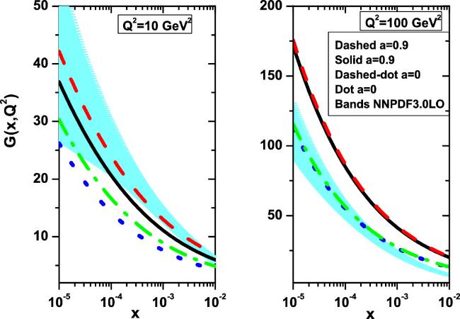
The results for the gluon distribution function (i.e., equation (30 )) in the CDM are presented based on the expansion point z = a over a wide range of x and μ2 = Q2 in Figures 1–2. The gluon distribution functions, with and without the rescaling variable (i.e., equation (3 ), $x\to x(1+4{m}_{c}^{2}/{\mu }^{2}))$ including the charm quark mass, are defined at Q2 = 10 and 100 GeV2. In figure 1, for Q2 = 10 and 100 GeV2, the gluon distribution with the rescaling variable at the expanding points a = 0.9 (solid curve, black) and a = 0 (dot curve, blue) and without the rescaling variable at the expanding points a = 0.9 (dashed curve, red) and a = 0 (dashed-dot curve, green) are compared with the CJ15LO [49] along with total errors (bands, cyan). In this figure, we observe that the gluon distribution at the expansion point a = 0.9 (with and without the rescaling variable) is comparable with the CJ15LO at Q2 = 10 GeV2 and at the expansion point a = 0 (with and without the rescaling variable) is comparable with the CJ15LO at Q2 = 100 GeV2 within the uncertainties errors across a wide range of x. In figure 2, the same results as in figure 1 are presented for the gluon distribution compared with the NNPDF3.0LO [50] along with total errors across a wide range of x. We observe that the results at low Q2 values are comparable with parametrization groups as the expansion point increases, and at large Q2 values, they are comparable at lower expansion points.
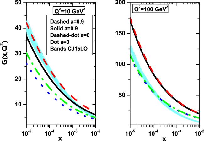
Figure 1. The gluon distribution function G(x, Q2) with the rescaling variable at the expanding points a = 0.9 (solid curve, black) and a = 0 (dot curve, blue) and without the rescaling variable at the expanding points a = 0.9 (dashed curve, red) and a = 0 (dashed-dot curve, green) compared with the CJ15LO [49] as accompanied with total errors (bands, cyan). |
According to the results5 at low and high Q2 values in figures 1 and 2, the longitudinal structure functions are obtained at fixed Q2 values (i.e., Q2 = 8.5 and 120 GeV2) and compared with the results of the H1 Collaboration [51] as a function of x. The longitudinal structure function extracted with and without the rescaling variable at Q2 values are in good agreement with experimental data compared to those in [51], with total errors shown in figure 3.
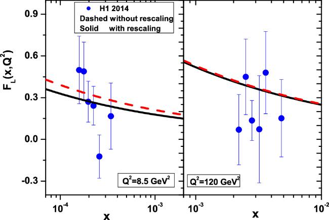
Figure 3. The longitudinal structure function FL(x, Q2) with (solid curves) and without (dashed curves) the rescaling variable plotted at fixed Q2 (left: Q2 = 8.5 GeV2, right: Q2 = 120 GeV2) as a function of x variable, compared with the H1 Collaboration data [51]. Experimental data (circles, H1 2014) are from the H1 Collaboration [51] as accompanied with total errors. |
The saturation scale with the x and a dependencies from the color-dipole models at the scale ${\mu }_{0}^{2}$ is given by
$\begin{eqnarray}{Q}_{s}^{2}(x,a)=\displaystyle \frac{3\pi {\mu }_{0}^{2}}{\alpha {\sigma }_{0}{R}_{{e}^{+}{e}^{-}}}\displaystyle \frac{\sigma ({W}_{0}^{2* })}{\mathrm{ln}\tfrac{\rho }{{\mu }_{0}^{* }}}{I}_{L}({\eta }_{0}^{* },{\mu }_{0}^{* }){G}_{L}({u}_{0}^{* }),\end{eqnarray}$
where this saturation scale connects the GBW form of the dipole cross-section with the CDP. In figure 4, we compare the saturation scales from the expansion points with the GBW model with charm from the Fits in table 1, as the coefficients σ0, λ and x0 are read from the first three rows of table 1 and the coefficients C and ${\mu }_{0}^{2}$ are read in the next two rows.6 We observe that the results with increases in the expansion point are close to the GBW model from Fits 0,1 in table 1. As a result, at x = 10−6 the saturation scale is order by $\mathrm{GBW}{| }_{{Q}_{s}^{2}\approx \,2-3\,{\mathrm{GeV}}^{2}}\gt \mathrm{Fit}\,0,1\ {| }_{{Q}_{s}^{2}\approx \,1-2\,{\mathrm{GeV}}^{2}}$ and at 10−4 < x < 10−2 the results are equal.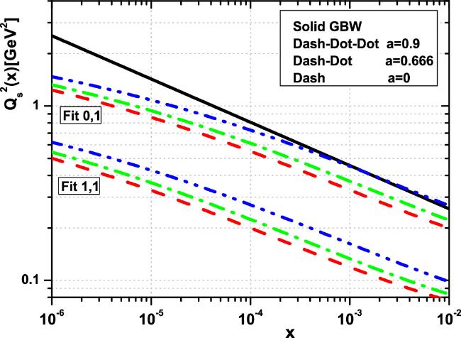
Figure 4. The saturation scale at the scale ${\mu }_{0}^{2}$ in the CDP model with the expansion points (a = 0, 0.666 and 0.9) with the parameters from the fits in table 1 compared with the GBW model (solid line) with the charm contribution. |
In figure 5, we show the ratio of dipole cross-sections (σdip/σ0) in accordance with the active flavor numbers and the quark mass effects. Quark mass effects are taken as zero for a massive quark i when ${\mu }^{2}\lt {m}_{i}^{2}$ and the quark treated as fully active when ${\mu }^{2}\gt {m}_{i}^{2}$. The ratio of dipole cross-sections is obtained, in figure 4, by solving equation (31 ) using the CDP ${xg}(x,{\mu }_{r}^{2})$ at the expansion points and compared with the GBW model with the heavy quark contributions. The results are shown for the selected dipole transverse size owing to the Fits 0–2. We observe that our results are sensitive to the expansion point when we compared with the GBW model with the heavy quarks contributions. The indicated values of r in figure 5 are in accordance with the heavy flavors of fit results in table 1. It is clear that for large values of r the two functions are very close, and they differ in the small r region where the running of the gluon distribution and its expansion starts to play a significant role. As a result, the DGLAP improved model with the gluon distribution in the CDP model can be extending to large values of Q2 (small dipole sizes).
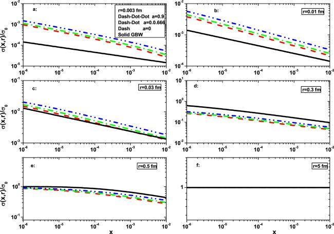
Figure 5. Comparison of the σdip(x, r)/σ0 obtained by solving equation ( |
In figure 6, we have calculated the r dependence, at low x (x = 10−3 and x = 10−6), of the ratio σdip(x, r)/σ0 (i.e., equation (31 )) owing to the expansion method. Results of calculations with Fits 1, 1 and 2, 2 (in table 1) and comparison with the GBW model with the charm and bottom contributions are presented in figure 6. We see in the left and right plots of figure 6 that for large values of r (r ≳ 1 fm) the two model results overlap while the CDP results lie below the GBW curves for the interval 0.04 fm ≲ r ≲ 1 fm. The deviation of the CDP results from the GBW model in the left and right plots of figure 6 are visible for r ≳ 0.04 fm, which is due to the running of the gluon distribution, is very visible (especially at very low x). Expanding of the gluon distribution around high and low values of z = a is close to the GBW results in the regions 0.04 fm ≲ r ≲ 1 fm and r ≲ 0.04 fm respectively. The uncertainties, in the left and right plots of figure 6, are due to the statistical errors in table 1 in the expansion point a = 0.666.
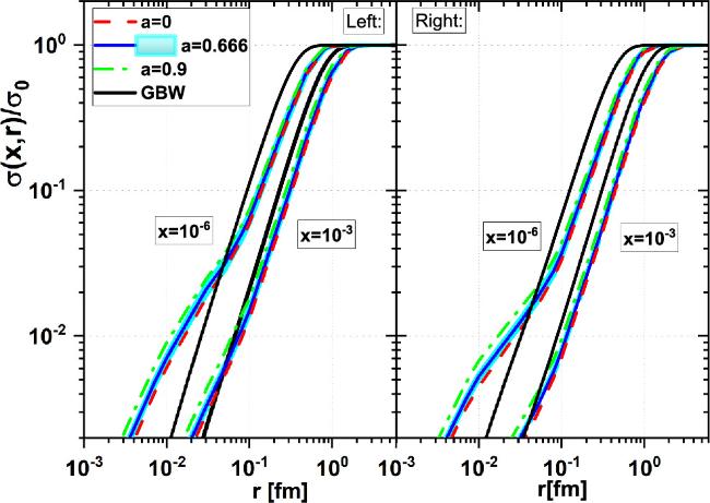
Figure 6. The ratio σdip(x, r)/σ0 according to the expansion points for x = 10−6 and 10−3 with the parameters compared with the GBW model: Left: Fit 1,1. Right: Fit 2,2. The uncertainties in the expansion point a = 0.666 are due to the statistical errors in table 1. |
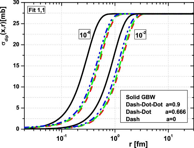
The form of the CDP results for the dipole cross-section σdip(x, r) (i.e., equation (31 )) at the expansion points (a = 0, 0.666 and 0.9) is shown in figure 7 for x = 10−6 and 10−2 with the parameters Fit 1, 1 in table 1. In figure 7, a comparison with the GBW model (with charm contribution) is done in a wide range of the dipole size r. The CDP results also show that the dipole cross-section features color transparency (i.e., σdip ∼ r2) at small r which is perturbative QCD phenomenon and for large r, saturation occurs (i.e., σdip ≃ σ0) [52, 53]. We see that the transition between two regimes occurs by decreasing transverse sizes with a decrease of x and this is visible in the large expansion points.
Figure 7. The dipole cross-section σdip(x, r) as a function of transverse dipole size r according to the expansion points for x = 10−6 and 10−2 with the parameters Fit 1, 1 compared with the GBW model with charm contribution. |
4. Conclusions
In summary, we have used an expansion method of the gluon density in the color-dipole formalism with heavy quark contributions and obtain the dipole cross-section in a wide range of the transverse dipole size r. The gluon density is obtained at an arbitrary point of expansion of $G(\tfrac{x}{1-z}){| }_{z\,=\,a}$, where it is dependent on the photoabsorption cross-section in the CDP. The associated CDP gluon density is valid for large as well as small r. The saturation line in the CDP model is dependent on the running of the gluon density on the (x, Q2)-plane and changed than the GBW model at very low x.
The dipole cross-sections in the improved saturation model are compared with the GBW model owing to the gluon density of the CDP model. The dipole cross-section is modified at small r than the GBW model by the gluon density with the Altarelli-Martinelli equation which is due to the pQCD phenomenon. The transition between the saturation and color transparency regions is dependent on the r, x and the expansion point in our model. We can see that this transition moves towards lower r as x decreases and the expansion point increases.
In conclusion, the color-dipole cross-section from unifying the color-dipole picture and improved saturation models gives a behavior in accordance to the pQCD result with respect to the expansion method.