


1. Introduction
2. Direct scattering
2.1. Direct scattering for λ
2.1.1. Lax pair, integral equations and analyticity of modified Jost solutions
(Time evolution) The Jost solutions ${{\rm{\Phi }}}_{\pm }\left(x,t;\lambda \right)$ satisfy Lax pair (3).
Because ${\rm{tr}}\left(L\right)=0$, Abel's identity tells us that ${\rm{\det }}{{\rm{\Phi }}}_{\pm }\left(x,t;\lambda \right)=1$, which means that ${{\rm{\Phi }}}_{\pm }\left(x,t;\lambda \right)$ are the fundamental matrix solutions. With the zero curvature equation ${L}_{t}-{A}_{x}+\left[L,A\right]=0$, we can find that $\frac{{\rm{d}}}{{\rm{d}}t}{{\rm{\Phi }}}_{\pm }\left(x,t;\lambda \right)-A{{\rm{\Phi }}}_{\pm }\left(x,t;\lambda \right)$ also satisfies Lax pair (
The behaviour of μ± as λ → 0 and $\left|\lambda \right|\to \infty $ has been studied in [23] via two matrix transformations which transform the modified spectral problem (9) denoted by $\left\{{\mu }_{\pm ,1},{\mu }_{\pm ,2}\right\}$ to two equivalent forms about the new normalized Jost functions $\left\{{m}_{\pm },{n}_{\pm }\right\}$ for small λ and $\left\{{\hat{m}}_{\pm },{\hat{n}}_{\pm }\right\}$ for large λ. They have proved rigorously that such two sets of new Jost functions about z := λ2 are analytic in ${{\mathbb{C}}}^{\pm }$ and continuous in ${{\mathbb{C}}}^{\pm }\cup {\mathbb{R}}$, given by lemma 5 in [23], where ${{\mathbb{C}}}^{\pm }$, respectively, corresponds to the upper and lower half-planes of the complex plane.
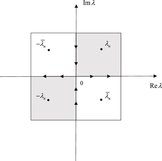
Figure 1. Complex λ-plane. The analytical regions D+ (grey) and D− (white) of the modified Jost solutions, discrete spectrum of the scattering problem and orientation of the contours for the RH problem. |
Suppose that $u\left(x,t\right),v\left(x,t\right)\in {L}^{1}\left({\mathbb{R}}\right)\cap {L}^{\infty }\left({\mathbb{R}}\right)$ and ${u}_{x}\left(x,t\right),{v}_{x}\left(x,t\right)\in {L}^{1}\left({\mathbb{R}}\right)$, the modified Jost solutions ${\mu }_{\pm }\left(x,t;\lambda \right)$ have the following properties:
(i) ${\mu }_{\pm }\left(x,t;\lambda \right)$ are unique for the modified Lax pair (9) satisfying ${\mu }_{\pm }\left(x,t;\lambda \right)\unicode{x0007E}I$ as x → ± ∞;
(ii) ${\mu }_{-,2}\left(x,t;\lambda \right)$, ${\mu }_{+,1}\left(x,t;\lambda \right)$ can be analytically extended to D+ and continuously extended to D+ ∪ Σ;
(iii) ${\mu }_{-,1}\left(x,t;\lambda \right)$, ${\mu }_{+,2}\left(x,t;\lambda \right)$ can be analytically extended to D− and continuously extended to D− ∪ Σ.
2.1.2. Scattering matrix and reflection coefficients
Suppose that $u\left(x,t\right),v\left(x,t\right)\in {L}^{1}\left({\mathbb{R}}\right)\cap {L}^{\infty }\left({\mathbb{R}}\right)$ and ${u}_{x}\left(x,t\right),{v}_{x}\left(x,t\right)\in {L}^{1}\left({\mathbb{R}}\right)$, ${s}_{11}\left(\lambda \right)$ can be analytically extended to D+ and continuously extended to D+ ∪ Σ, ${s}_{22}\left(\lambda \right)$ can be analytically extended to D−and continuously extended to D− ∪ Σ, while both ${s}_{12}\left(\lambda \right)$ and ${s}_{21}\left(\lambda \right)$ are only continuous in Σ.
2.1.3. Symmetries
There exist two kinds of symmetries for $L\left(x,t;\lambda \right)$, $A\left(x,t;\lambda \right)$, ${\mu }_{\pm }\left(x,t;\lambda \right)$, ${{\rm{\Phi }}}_{\pm }\left(x,t;\lambda \right)$, $S\left(\lambda \right)$ and $\rho \left(\lambda \right)$:
(i) The first symmetry $\left(\lambda \mapsto \overline{\lambda }\right)$
(ii) The second symmetry $\left(\lambda \mapsto -\overline{\lambda }\right)$
2.1.4. Asymptotic behaviors as λ → ∞
The asymptotic behaviors of the modified Jost solutions and $S\left(\lambda \right)$ are given, respectively, as
This proposition is consistent with equations (2.22) and (3.15) in [23].
2.2. Direct scattering for ω
2.2.1. Lax pair, integral equations and analyticity of modified Jost solutions
Suppose that $u\left(x,t\right),v\left(x,t\right)\in {L}^{1}\left({\mathbb{R}}\right)\cap {L}^{\infty }\left({\mathbb{R}}\right)$, ${u}_{x}\left(x,t\right),{v}_{x}\left(x,t\right)\in {L}^{1}\left({\mathbb{R}}\right)$ and ${\widetilde{\mu }}_{\pm ,j}\left(x,t;\omega \right)$ is the j-th column of the matrix functions ${\widetilde{\mu }}_{\pm }\left(x,t;\omega \right)$ $\left(j=1,2\right)$. Then, the modified Jost solutions ${\widetilde{\mu }}_{\pm }\left(x,t;\omega \right)$ have the following properties:
(i) ${\widetilde{\mu }}_{\pm }\left(x,t;\omega \right)$ are unique for the modified Lax pair (29) satisfying ${\widetilde{\mu }}_{\pm }\left(x,t;\omega \right)\unicode{x0007E}I$ as x → ± ∞;
(ii) ${\widetilde{\mu }}_{-,2}\left(x,t;\omega \right)$, ${\widetilde{\mu }}_{+,1}\left(x,t;\omega \right)$ can be analytically extended to D− and continuously extended to D− ∪ Σ;
(iii) ${\widetilde{\mu }}_{-,1}\left(x,t;\omega \right)$, ${\widetilde{\mu }}_{+,2}\left(x,t;\omega \right)$ can be analytically extended to D+ and continuously extended to D+ ∪ Σ.
2.2.2. Scattering matrix and reflection coefficients
Suppose that $u\left(x,t\right),v\left(x,t\right)\in {L}^{1}\left({\mathbb{R}}\right)\cap {L}^{\infty }\left({\mathbb{R}}\right)$ and ${u}_{x}\left(x,t\right),{v}_{x}\left(x,t\right)\in {L}^{1}\left({\mathbb{R}}\right)$, ${\widetilde{s}}_{11}\left(\omega \right)$ can be analytically extended to D−and continuously extended to D− ∪ Σ, ${\widetilde{s}}_{22}\left(\omega \right)$ can be analytically extended to D+ and continuously extended to D+ ∪ Σ, while both ${\widetilde{s}}_{12}\left(\omega \right)$ and ${\widetilde{s}}_{21}\left(\omega \right)$ are only continuous in Σ.
2.2.3. Symmetries
There exist two kinds of symmetries for $\widetilde{L}(x,t;\omega )$, $\widetilde{A}(x,t;\omega )$, ${\widetilde{\mu }}_{\pm }(x,t;\omega )$, ${\widetilde{{\rm{\Phi }}}}_{\pm }(x,t;\omega )$, $\widetilde{S}(\omega )$ and $\widetilde{\rho }(\omega )$:
(i) The first symmetry $\left(\omega \mapsto \overline{\omega }\right)$
(ii) The second symmetry $\left(\omega \mapsto -\overline{\omega }\right)$
2.2.4. Asymptotic behaviors as ω → ∞
3. Inverse scattering
3.1. Inverse scattering for λ
3.1.1. Matrix RH problem
3.1.2. Residue conditions and reconstruction formula
3.1.3. Trace formulas
3.1.4. Solution v for the reflectionless case
3.2. Inverse scattering for ω
3.2.1. Matrix RH problem
3.2.2. Residue conditions and reconstruction formula
3.2.3. Trace formulas
3.2.4. Solution u for the reflectionless case
4. Soliton solutions and asymptotic analysis
4.1. One-soliton solutions
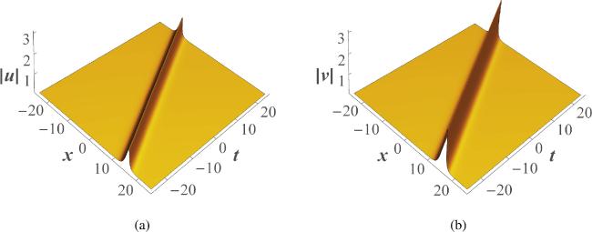
Figure 2. 3D plots of the one-soliton solutions ( |
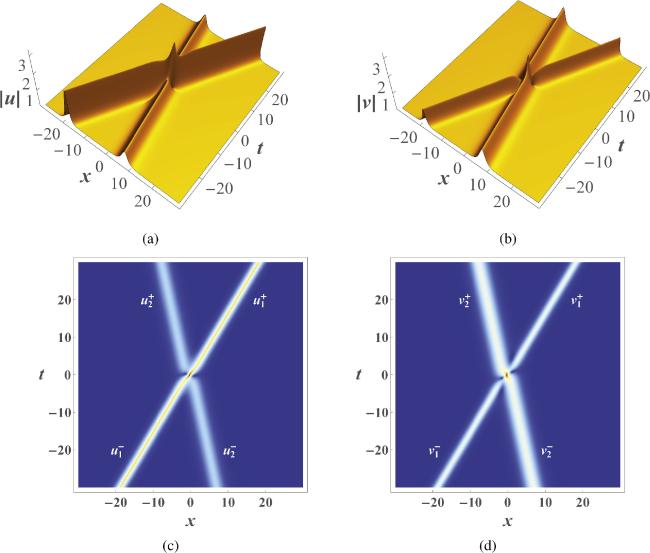
Figure 3. (a) and (b): 3D plots of the two-soliton solutions in the components u and v with ${\xi }_{1}=\frac{1}{2}+\frac{1}{2}{\rm{i}}$, ${\xi }_{2}=1+\frac{1}{2}{\rm{i}}$, b1 = 1 + i and b2 = 1 + i; (c) and (d): Density plots of (a) and (b). |
4.2. Two-soliton solutions
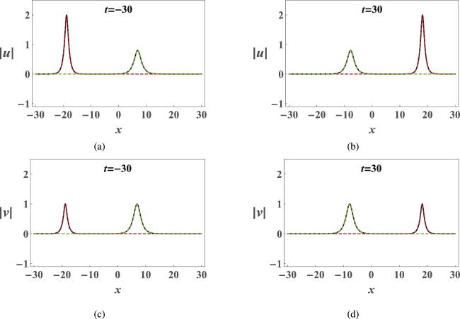
Figure 4. Comparison of the asymptotic solitons ${u}_{j}^{\pm }$ and ${v}_{j}^{\pm }$ ( red and green dashed for j = 1 and j = 2, respectively) with the exact solutions (black solid) at different t with ${\xi }_{1}=\frac{1}{2}+\frac{1}{2}{\rm{i}}$, ${\xi }_{2}=1+\frac{1}{2}{\rm{i}}$, b1 = 1 + i and b2 = 1 + i. |
4.3. Bound-state solutions
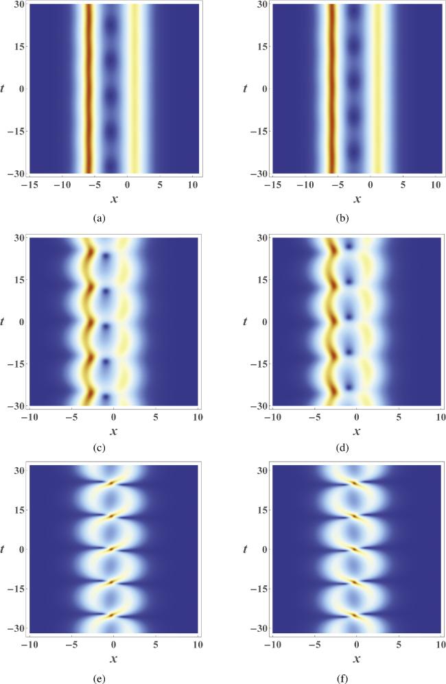
(i) If $\left|\left|{b}_{1}\right|-\left|{b}_{2}\right|\right|\gg 0$, the two solitons are well separated and their relative distance changes very little as the time evolves, so that the interaction force is quite weak (see figures 5(a) and 5(b)).
(ii) If $\left|\left|{b}_{1}\right|-\left|{b}_{2}\right|\right|\gt 0$, the relative distance between two solitons changes periodically but it will not decrease to 0, which means that they never collide at one point (see figures 5(c) and 5(d)).
(iii) If $\left|{b}_{1}\right|=\left|{b}_{2}\right|$, the two solitons collide periodically and form a series of transient waves with large amplitudes at interaction points, so that the strength of soliton interaction is strong, as shown in figures 5(e) and 5(f).
Figure 5. Density plots for three different two-soliton bound states in the components u (left figures) and v (right figures), where the parameters are selected as: ${\xi }_{1}=\frac{\sqrt{2}}{2}+\frac{\sqrt{2}}{2}{\rm{i}}$, ${\xi }_{2}=\frac{\sqrt{3}}{2}+\frac{1}{2}{\rm{i}}$, and b1 = 70 + 70i and b2 = 1 + i for (a) and (b); b1 = 4 + 4i and b2 = 1 + i for (c) and (d); b1 = 1 + i and b2 = 1 + i for (e) and (f). |