


1. Introducing
Quantum entanglement [1–3] is one of the most fascinating phenomena in quantum mechanics. Entangled states are useful for exploring non-locality, bolstering quantum mechanics against theories of local hidden variables. Morerover, entangled states are also a key resource for quantum information processing tasks [4–6]. It is widely used in quantum teleportation [7–9], quantum key distribution [10–12], quantum cryptography [2, 13–15], quantum computing [16, 17] and so on. So far, many theoretical and experimental schemes have been proposed for preparing and converting entangled states [18–28]. As we know, each type of entangled state has its own characteristics, therefore, exploring the conversion between different types of entangled states has become a fascinating research direction in quantum mechanics.
On the other hand, neutral atoms are regarded as ideal candidates for quantum information processing due to stabilized atomic hyperfine energy states and extremely large dipole moments, which are particularly suitable for encoding logic quantum bits [29–33]. When an atom is excited to the high Rydberg state, the strong dipole–dipole interaction or van der Waals interaction will significantly shift its surrounding atomic energy levels of Rydberg states, this leads to the emergent energy level shift term in the Hamiltonian. Mathematically, it is because of this energy level shift term that a series of interesting physical phenomena arise, such as the Rydberg blocking effect [34–37] and the Rydberg anti-blocking effect [38–42]. In addition, it can be a very interesting tool to simplify the dynamics of systems, as well as, providing researchers with brand new ideas. There are a lot of excellent studies to realize conversions between different entangled states using neutral atoms [18–20, 43–45]. It is worth noting that Zheng et al [18] proposed a protocol for the one-step interconversion between the Greenberger–Horne–Zeilinger (GHZ) state and the W state with deterministic success probabilities by utilizing a Rydberg mechanism to structure nonlocal operation. It has been demonstrated that the two types of entangled states cannot be interconverted only by local operations and classical communication. We consider that since a deterministic interconversion between the GHZ and W states can be realized in one step by utilizing a Rydberg mechanism to structure nonlocal operation [18], it might also be possible to realize the deterministic conversion between other entangled states in one step.
We focus on another type of Knill–Laflamme–Milburn (KLM) entangled state [46]. The KLM state was introduced mainly in the linear optical quantum computing scheme proposed by Knill, Laflamme and Milburn. It can effectively reduce the operation error rate and improve the implementation efficiency of quantum algorithms. Subsequently, not limited to optical systems, Popescu et al [47] demonstrated that the atomic KLM can also be used for computation. Since then, considerable efforts have been invested in preparing KLM-type quantum entanglement using various physical platforms [48–54], such as linear optics, atom-cavity quantum electrodynamics, nonlinear cross-Kerr media, and artificial atoms. The n-qubit KLM state is expressed as
$\begin{eqnarray}| \mathrm{KLM}\rangle =\displaystyle \sum _{k=0}^{n}{\alpha }_{n}| 1{\rangle }^{k}| 0{\rangle }^{n-k},\end{eqnarray}$
where ${\alpha }_{n}=1/\sqrt{n+1}$, is the normalization coefficient for maximal entanglement.After extensive literature review, although many schemes have been proposed for directly preparing the GHZ state or KLM state in an atomic system [25, 53–57] and a scheme for converting the GHZ state and KLM state in optical systems [28], we found that research on the conversion between the GHZ state and KLM state in neutral atomic systems has not been reported. In the present work, inspired by the previous schemes, we propose a scheme to deterministic implement interconversion between the GHZ state and KLM state with one-step. The scheme's physical model features three neutral atoms with Rydberg capabilities, positioned in a triangular configuration, the original Hamiltonian is simplified to an effective four-energy system through meticulously crafted detunings and approximation technique. Then, we combine the effective Hamiltonian and Lie-transform-based pulse design [58, 59] to realize the interconversion of the GHZ state and KLM state.
The paper is organized as follows. In section 2 , we introduce the physical model and simplify the system to an effective four-energy level system. In section 3 , we briefly review the methods for Lie-transform-based pulse design, subsequently, we combine the effective Hamiltonian and Lie-transform-based pulse design to structure control pulses to realize the interconversion between the GHZ state and KLM state. Next, in section 4 , we give numerical simulations and analyses for the scheme, and further discuss the robustness about a number of imperfections. Lastly, a summary is given in section 5 .
2. Physical model
We consider three same neutral atoms confined within three distinct microscopic dipole traps, and arranged in a triangular configuration as show in figure 1(a), V represents the van der Waals or dipole–dipole interaction between different atoms that are in Rydberg states. The energy levels of the three neutral atoms with Rydberg states as shown in figure 1(b), each atomic level includes a ground state ∣0⟩ and a Rydberg state ∣r⟩. The transition ∣0⟩k ↔ ∣r⟩k is driven by classical laser fields with Rabi frequencies Ωk, whose detunings are δk, where k denotes the kth atom in the physical model. In the interaction picture, the Hamiltonian of the physical model takes the form(ℏ = 1)
$\begin{eqnarray}\begin{array}{rcl}H(t) & = & \displaystyle \sum _{k=1}^{3}{{\rm{\Omega }}}_{k}{{\rm{e}}}^{-{\rm{i}}{\delta }_{k}t}| r{\rangle }_{k}\langle 0| \\ & & +{\rm{H.c.}}+V\displaystyle \sum _{k=2}^{3}\displaystyle \sum _{k^{\prime} =1}^{k-1}| rr{\rangle }_{k^{\prime} k}\langle rr| .\end{array}\end{eqnarray}$
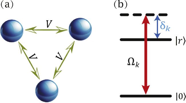
Figure 1. (a) Schematic illustration of system. Three identical neutral atoms confined within three separate microscopic dipole traps, arranged in a triangular configuration. (b) The energy levels configuration for the single atom. |
To improve the understanding and facilitate discussion of the physical model, we rewrite the Hamiltonian in triatomic basis vectors
$\begin{eqnarray}\begin{array}{rcl}H & = & {{\rm{\Omega }}}_{1}{{\rm{e}}}^{-{\rm{i}}{\delta }_{1}t}| r00\rangle \langle 000| +{{\rm{\Omega }}}_{2}{{\rm{e}}}^{-{\rm{i}}{\delta }_{2}t}| 0r0\rangle \langle 000| \\ & & +{{\rm{\Omega }}}_{3}{{\rm{e}}}^{-{\rm{i}}{\delta }_{3}t}| 00r\rangle \langle 000| +{{\rm{\Omega }}}_{2}{{\rm{e}}}^{-{\rm{i}}{\delta }_{2}t}| rr0\rangle \langle r00| \\ & & +{{\rm{\Omega }}}_{3}{{\rm{e}}}^{-{\rm{i}}{\delta }_{3}t}| r0r\rangle \langle r00| +{{\rm{\Omega }}}_{1}{{\rm{e}}}^{-{\rm{i}}{\delta }_{1}t}| rr0\rangle \langle 0r0| \\ & & +{{\rm{\Omega }}}_{3}{{\rm{e}}}^{-{\rm{i}}{\delta }_{3}t}| 0rr\rangle \langle 0r0| +{{\rm{\Omega }}}_{1}{{\rm{e}}}^{-{\rm{i}}{\delta }_{1}t}| r0r\rangle \langle 00r| \\ & & +{{\rm{\Omega }}}_{2}{{\rm{e}}}^{-{\rm{i}}{\delta }_{2}t}| 0rr\rangle \langle 00r| +{{\rm{\Omega }}}_{3}{{\rm{e}}}^{-{\rm{i}}{\delta }_{3}t}| rrr\rangle \langle rr0| \\ & & +{{\rm{\Omega }}}_{2}{{\rm{e}}}^{-{\rm{i}}{\delta }_{2}t}| rrr\rangle \langle r0r| +{{\rm{\Omega }}}_{1}{{\rm{e}}}^{-{\rm{i}}{\delta }_{1}t}| rrr\rangle \langle 0rr| +{\rm{H.c.}}\\ & & +V| rr0\rangle \langle rr0| +V| r0r\rangle \langle r0r| \\ & & +V| 0rr\rangle \langle 0rr| +3V| rrr\rangle \langle rrr| .\end{array}\end{eqnarray}$
From equation (3 ), we can easily observe the energy level shifts caused by Rydberg states, this energy level shift is 3 ) in new picture becomes
$\begin{eqnarray}\begin{array}{rcl}{H}_{V} & = & V| rr0\rangle \langle rr0| +V| r0r\rangle \langle r0r| \\ & & +V| 0rr\rangle \langle 0rr| +3V| rrr\rangle \langle rrr| .\end{array}\end{eqnarray}$
Next, we define a rotating frame with a unitary operator ${ \mathcal R }=\exp (-{\rm{i}}{H}_{V}t)$, and move into the new picture through $\begin{eqnarray}H^{\prime} ={{ \mathcal R }}^{\dagger }H{ \mathcal R }-{\rm{i}}{{ \mathcal R }}^{\dagger }\dot{{ \mathcal R }}.\end{eqnarray}$
So, the Hamiltonian ( $\begin{eqnarray}\begin{array}{rcl}H^{\prime} & = & {{\rm{\Omega }}}_{1}{{\rm{e}}}^{-{\rm{i}}{\delta }_{1}t}| r00\rangle \langle 000| +{{\rm{\Omega }}}_{2}{{\rm{e}}}^{-{\rm{i}}{\delta }_{2}t}| 0r0\rangle \langle 000| \\ & & +{{\rm{\Omega }}}_{3}{{\rm{e}}}^{-{\rm{i}}{\delta }_{3}t}| 00r\rangle \langle 000| +{{\rm{\Omega }}}_{2}{{\rm{e}}}^{-{\rm{i}}({\delta }_{2}-V)t}| rr0\rangle \langle r00| \\ & & +{{\rm{\Omega }}}_{3}{{\rm{e}}}^{-{\rm{i}}({\delta }_{3}-V)t}| r0r\rangle \langle r00| +{{\rm{\Omega }}}_{1}{{\rm{e}}}^{-{\rm{i}}({\delta }_{1}-V)t}| rr0\rangle \\ & & \times \langle 0r0| +{{\rm{\Omega }}}_{3}{{\rm{e}}}^{-{\rm{i}}({\delta }_{3}-V)t}| 0rr\rangle \langle 0r0| \\ & & +{{\rm{\Omega }}}_{1}{{\rm{e}}}^{-{\rm{i}}({\delta }_{1}-V)t}| r0r\rangle \langle 00r| +{{\rm{\Omega }}}_{2}{{\rm{e}}}^{-{\rm{i}}({\delta }_{2}-V)t}| 0rr\rangle \\ & & \times \langle 00r| +{{\rm{\Omega }}}_{3}{{\rm{e}}}^{-{\rm{i}}({\delta }_{3}-2V)t}| rrr\rangle \langle rr0| \\ & & +{{\rm{\Omega }}}_{2}{{\rm{e}}}^{-{\rm{i}}({\delta }_{2}-2V)t}| rrr\rangle \langle r0r| +{{\rm{\Omega }}}_{1}{{\rm{e}}}^{-{\rm{i}}({\delta }_{1}-2V)t}| rrr\rangle \\ & & \times \langle 0rr| +{\rm{H.c.}}\end{array}\end{eqnarray}$
If we encode the logical '0' with ground state ∣0⟩ and use the Rydberg state ∣r⟩ to encode logical '1', the three-particle KLM state and GHZ state has the following form 6 ), it may accomplish the preparation of the GHZ state and KLM state, as well as enable their interconversion. Based on this consideration, we set the detuning of the Rabi frequencies are δ1 = 0, δ2 = V, δ3 = 2V, respectively, then the Hamiltonian (6 ) becomes
$\begin{eqnarray}| {\rm{KLM}}\rangle =\frac{1}{2}(| 000\rangle +| r00\rangle +| rr0\rangle +| rrr\rangle ),\end{eqnarray}$
and $\begin{eqnarray}| {\rm{GHZ}}\rangle =\frac{1}{\sqrt{2}}(| 000\rangle +| rrr\rangle ).\end{eqnarray}$
We considered that if constructing an evolutionary space within {∣000⟩, ∣r00⟩, ∣rr0⟩, ∣rrr⟩} from equation ( $\begin{eqnarray}\begin{array}{rcl}H^{\prime} & = & {{\rm{\Omega }}}_{1}| r00\rangle \langle 000| +{{\rm{\Omega }}}_{2}{{\rm{e}}}^{-{\rm{i}}Vt}| 0r0\rangle \langle 000| \\ & & +{{\rm{\Omega }}}_{3}{{\rm{e}}}^{-{\rm{i}}2Vt}| 00r\rangle \langle 000| +{{\rm{\Omega }}}_{2}| rr0\rangle \langle r00| \\ & & +{{\rm{\Omega }}}_{3}{{\rm{e}}}^{-{\rm{i}}Vt}| r0r\rangle \langle r00| +{{\rm{\Omega }}}_{1}{{\rm{e}}}^{{\rm{i}}Vt}| rr0\rangle \langle 0r0| \\ & & +{{\rm{\Omega }}}_{3}{{\rm{e}}}^{-{\rm{i}}Vt}| 0rr\rangle \langle 0r0| \\ & & +{{\rm{\Omega }}}_{1}{{\rm{e}}}^{{\rm{i}}Vt}| r0r\rangle \langle 00r| \\ & & +{{\rm{\Omega }}}_{2}| 0rr\rangle \langle 00r| +{{\rm{\Omega }}}_{3}| rrr\rangle \langle rr0| +{{\rm{\Omega }}}_{2}{{\rm{e}}}^{{\rm{i}}Vt}| rrr\rangle \\ & & \times \langle r0r| +{{\rm{\Omega }}}_{1}{{\rm{e}}}^{{\rm{i}}2Vt}| rrr\rangle \langle 0rr| +{\rm{H.c.}}\end{array}\end{eqnarray}$
Through neglecting highly frequent oscillations under the condition $V\gg {\rm{Max}}\{{{\rm{\Omega }}}_{1},{{\rm{\Omega }}}_{2},{{\rm{\Omega }}}_{3}\}$, the effective Hamiltonian is simplified as 10 ), we can find that if the initial state belongs to the evolutionary subspace {∣000⟩, ∣r00⟩, ∣rr0⟩, ∣rrr⟩}, the evolution of the system will remain within this evolutionary subspace. That is to say, in this case, the term Ω2∣0rr⟩⟨00r∣ and its Hermitian conjugate are decoupled in the effective Hamiltonian (10 ), so the effective Hamiltonian becomes
$\begin{eqnarray}\begin{array}{rcl}H{{\prime} }_{{\rm{eff}}} & = & {{\rm{\Omega }}}_{1}| r00\rangle \langle 000| +{{\rm{\Omega }}}_{2}| rr0\rangle \langle r00| +{{\rm{\Omega }}}_{2}| 0rr\rangle \\ & & \times \langle 00r| +{{\rm{\Omega }}}_{3}| rrr\rangle \langle rr0| +{\rm{H.c.}}\end{array}\end{eqnarray}$
From equation ( $\begin{eqnarray}\begin{array}{rcl}{H}_{{\rm{eff}}} & = & {{\rm{\Omega }}}_{1}| r00\rangle \langle 000| +{{\rm{\Omega }}}_{2}| rr0\rangle \langle r00| \\ & & +{{\rm{\Omega }}}_{3}| rrr\rangle \langle rr0| +{\rm{H.c.}}\end{array}\end{eqnarray}$
3. Control field design through inverse Hamiltonian engineering based on Lie transforms
3.1. Lie transforms-based pulse design
First of all, we briefly describe the Lie-transform-based pulse design [59], for a quantum system with time-dependent interaction, assuming the Hamiltonian is expressed as follows 15 ), there are N parameters {θ1, θ2, ⋯ θn}, corresponding to N control parameters {λ1, λ2, ⋯ λn}, it opens up the possibility for designing control parameters.
$\begin{eqnarray}{ \mathcal H }(t)=\displaystyle \sum _{j=1}^{N}{\lambda }_{j}(t){A}_{j},\end{eqnarray}$
where the parameters λj(t) are time-dependent. Additionally, {Aj} is a set of Hermitian generators spanning a Lie algebra and {Aj} as the basis of an N-dimensional Hilbert space ${ \mathcal A }$. A set of Lie transforms $\{{{\mathscr{L}}}_{j}\}$ is defined and each function ${{\mathscr{L}}}_{j}$ acting on any vector $A\in { \mathcal A }$ is $\begin{eqnarray}{{\mathscr{L}}}_{j}(A)={{\rm{e}}}^{{\rm{i}}{\theta }_{j}(t){A}_{j}}A{{\rm{e}}}^{-{\rm{i}}{\theta }_{j}(t){A}_{j}},\end{eqnarray}$
where parameter θj is time-dependent and designed. Since the rotation ${{\rm{e}}}^{{\rm{i}}{\theta }_{j}(t){A}_{j}}$ can transform the Hamiltonian from a picture to another picture, it define picture transform ${{\mathscr{P}}}_{j}$ acting on ${ \mathcal H }(t)$ as $\begin{eqnarray}\begin{array}{l}{{\mathscr{P}}}_{j}({ \mathcal H })\,=\,{{\rm{e}}}^{{\rm{i}}{\theta }_{j}(t){A}_{j}}{ \mathcal H }(t){{\rm{e}}}^{-{\rm{i}}{\theta }_{j}(t){A}_{j}}\\ \,-\,{\rm{i}}{{\rm{e}}}^{{\rm{i}}{\theta }_{j}(t){A}_{j}}\frac{{\rm{d}}}{{\rm{d}}t}\left({{\rm{e}}}^{-{\rm{i}}{\theta }_{j}(t){A}_{j}}\right)\,=\,{{\mathscr{L}}}_{j}({ \mathcal H })-{\dot{\theta }}_{j}(t){A}_{j},\end{array}\end{eqnarray}$
hence, when considering the compound picture transform ${{\mathscr{P}}}_{N}\circ \cdots \circ {{\mathscr{P}}}_{2}\circ {{\mathscr{P}}}_{1}$ on Hamiltonian ${ \mathcal H }$, we can obtain the equation $\begin{eqnarray}\begin{array}{rcl}{{\mathscr{P}}}_{N}\circ \cdots \circ {{\mathscr{P}}}_{2}\circ {{\mathscr{P}}}_{1}({ \mathcal H }) & = & {{\mathscr{L}}}_{N}\circ \cdots \circ {{\mathscr{L}}}_{2}\circ {{\mathscr{L}}}_{1}({ \mathcal H })\\ & & -{\dot{\theta }}_{1}{{\mathscr{L}}}_{N}\circ \cdots \circ {{\mathscr{L}}}_{3}\circ {{\mathscr{L}}}_{2}({A}_{1})\\ & & -{\dot{\theta }}_{2}{{\mathscr{L}}}_{N}\circ \cdots \circ {{\mathscr{L}}}_{4}\circ {{\mathscr{L}}}_{3}({A}_{2})\\ & & -\cdots \\ & & -{\dot{\theta }}_{N-2}(t){{\mathscr{L}}}_{N}\circ {{\mathscr{L}}}_{N-1}({A}_{N-2})\\ & & -{\dot{\theta }}_{N-1}(t){{\mathscr{L}}}_{N}({A}_{N-1})\\ & & -{\dot{\theta }}_{N}(t){A}_{N}.\end{array}\end{eqnarray}$
It can be observed that equation (On the other hand, the quantum state evolving from the initial state ψ(t0) is controlled by the evolution operator U and satisfies the Schrödinger equation 15 ) and equation (18 ), when considering ${{\mathscr{P}}}_{N}\circ \cdots \circ {{\mathscr{P}}}_{2}\circ {{\mathscr{P}}}_{1}({ \mathcal H })=0$, we can find the relationship between the evolution operator U and the compound picture view transformation. Thus, if the initial time is t0, the evolution operator of the system is 18 )
$\begin{eqnarray}{\rm{i}}\frac{\partial }{\partial t}(U\psi ({t}_{0}))={ \mathcal H }U\psi ({t}_{0}).\end{eqnarray}$
Through the arbitrariness of ψ(t0), we can obtain $\begin{eqnarray}{\rm{i}}\dot{U}={ \mathcal H }U.\end{eqnarray}$
It is equivalent to $\begin{eqnarray}0={U}^{\dagger }{ \mathcal H }U-{\rm{i}}{U}^{\dagger }\dot{U},\end{eqnarray}$
comparison of equation ( $\begin{eqnarray}\begin{array}{rcl}U(t) & = & {{\rm{e}}}^{-{\rm{i}}{\theta }_{1}(t){A}_{1}}{{\rm{e}}}^{-{\rm{i}}{\theta }_{2}(t){A}_{2}}\cdots {{\rm{e}}}^{-{\rm{i}}{\theta }_{N}(t){A}_{N}}\\ & & \times {{\rm{e}}}^{{\rm{i}}{\theta }_{N}({t}_{0}){A}_{N}}{{\rm{e}}}^{{\rm{i}}{\theta }_{N-1}({t}_{0}){A}_{N-1}}\cdots {{\rm{e}}}^{{\rm{i}}{\theta }_{1}({t}_{0}){A}_{1}}.\end{array}\end{eqnarray}$
We can derive the following equation from equation ( $\begin{eqnarray}\begin{array}{rcl}{{\mathscr{L}}}_{N}\circ \cdots \circ {{\mathscr{L}}}_{2}\circ {{\mathscr{L}}}_{1}({ \mathcal H }) & = & {\dot{\theta }}_{1}(t){{\mathscr{L}}}_{N}\circ \cdots \circ {{\mathscr{L}}}_{3}\circ {{\mathscr{L}}}_{2}({A}_{1})\\ & & +{\dot{\theta }}_{2}(t){{\mathscr{L}}}_{N}\circ \cdots \circ {{\mathscr{L}}}_{4}\circ {{\mathscr{L}}}_{3}\\ & & +\cdots \\ & & +{\dot{\theta }}_{N-2}(t){{\mathscr{L}}}_{N}\circ {{\mathscr{L}}}_{N-1}({A}_{N-2})\\ & & +{\dot{\theta }}_{N-1}(t){{\mathscr{L}}}_{N}({A}_{N-1})\\ & & +{\dot{\theta }}_{N}(t){A}_{N}.\end{array}\end{eqnarray}$
In general, by designing the parameter θ1, θ2 ⋯ θN within the evolution operator, we can control the evolution of the system's state to achieve the desired state, and the choice of parameter θ1, θ2 ⋯ θN also allows to inversely determine the control parameter λ1, λ2, ⋯ λn.3.2. Interconversion of GHZ state and KLM state
In this section, we combine effective Hamiltonian equation (11 ) and Lie-transform-based pulse design to create control pulses. We aim to obtain evolution operators in real form and consider them in conjunction with the effective Hamiltonian, thus we choose the following generator 20 ), we can derive 19 ), when we set θk(t0) =0 (k = 1, 2 ⋯ , 6) in initial time t0, the real evolution operator of effective Hamiltonian (11 ) can be written
$\begin{eqnarray}\begin{array}{rcl}{A}_{1} & = & {\rm{i}}| {\zeta }_{2}\rangle \langle {\zeta }_{1}| -{\rm{i}}| {\zeta }_{1}\rangle \langle {\zeta }_{2}| ,\\ {A}_{2} & = & {\rm{i}}| {\zeta }_{4}\rangle \langle {\zeta }_{3}| -{\rm{i}}| {\zeta }_{3}\rangle \langle {\zeta }_{4}| ,\\ {A}_{3} & = & {\rm{i}}| {\zeta }_{2}\rangle \langle {\zeta }_{3}| -{\rm{i}}| {\zeta }_{3}\rangle \langle {\zeta }_{2}| ,\\ {A}_{4} & = & {\rm{i}}| {\zeta }_{4}\rangle \langle {\zeta }_{1}| -{\rm{i}}| {\zeta }_{1}\rangle \langle {\zeta }_{4}| ,\\ {A}_{5} & = & {\rm{i}}| {\zeta }_{3}\rangle \langle {\zeta }_{1}| -{\rm{i}}| {\zeta }_{1}\rangle \langle {\zeta }_{3}| ,\\ {A}_{6} & = & {\rm{i}}| {\zeta }_{4}\rangle \langle {\zeta }_{2}| -{\rm{i}}| {\zeta }_{2}\rangle \langle {\zeta }_{4}| ,\end{array}\end{eqnarray}$
with ∣ζ1⟩ = ∣000⟩, ∣ζ2⟩ = ∣r00⟩, ∣ζ3⟩ = ∣rr0⟩, ∣ζ4⟩ = ∣rrr⟩. Obviously, the effective Hamiltonian is $\begin{eqnarray}{H}_{{\rm{eff}}}={\rm{\Omega }}{{\prime} }_{1}{A}_{1}+{\rm{\Omega }}{{\prime} }_{2}{A}_{3}+{\rm{\Omega }}{{\prime} }_{3}{A}_{2},\end{eqnarray}$
where ${{\rm{\Omega }}}_{1}={\rm{i}}{\rm{\Omega }}{{\prime} }_{1}$, ${{\rm{\Omega }}}_{2}=-{\rm{i}}{\rm{\Omega }}{{\prime} }_{2}$, ${{\rm{\Omega }}}_{3}={\rm{i}}{\rm{\Omega }}{{\prime} }_{3}$. From equation ( $\begin{eqnarray}\begin{array}{rcl}{H}_{{\rm{eff}}} & = & {\dot{\theta }}_{1}(t){A}_{1}+{\dot{\theta }}_{2}(t){{\mathscr{L}}}_{1}^{-1}{A}_{2}+{\dot{\theta }}_{3}(t){{\mathscr{L}}}_{1}^{-1}{{\mathscr{L}}}_{2}^{-1}{A}_{3}\\ & & +{\dot{\theta }}_{4}(t){{\mathscr{L}}}_{1}^{-1}{{\mathscr{L}}}_{2}^{-1}{{\mathscr{L}}}_{3}^{-1}{A}_{4}\\ & & +{\dot{\theta }}_{5}(t){{\mathscr{L}}}_{1}^{-1}{{\mathscr{L}}}_{2}^{-1}{{\mathscr{L}}}_{3}^{-1}{{\mathscr{L}}}_{4}^{-1}{A}_{5}\\ & & +{\dot{\theta }}_{6}(t){{\mathscr{L}}}_{1}^{-1}{{\mathscr{L}}}_{2}^{-1}{{\mathscr{L}}}_{3}^{-1}{{\mathscr{L}}}_{4}^{-1}{{\mathscr{L}}}_{5}^{-1}{A}_{6},\end{array}\end{eqnarray}$
then, the forms of parameters in control fields can be obtained $\begin{eqnarray}\begin{array}{rcl}{\rm{\Omega }}{{\prime} }_{1} & = & {\dot{\theta }}_{1}+{\dot{\theta }}_{5}\cos {\theta }_{4}\sin {\theta }_{3}+{\dot{\theta }}_{6}\cos {\theta }_{3}\sin {\theta }_{4},\\ {\rm{\Omega }}{{\prime} }_{2} & = & {\dot{\theta }}_{3}\cos {\theta }_{1}\cos {\theta }_{2}+{\dot{\theta }}_{4}\sin {\theta }_{1}\sin {\theta }_{2}\\ & & -{\dot{\theta }}_{5}\cos {\theta }_{2}\cos {\theta }_{3}\cos {\theta }_{4}\sin {\theta }_{1}\\ & & -{\dot{\theta }}_{5}\cos {\theta }_{1}\sin {\theta }_{2}\sin {\theta }_{3}\sin {\theta }_{4}\\ & & +{\dot{\theta }}_{6}\cos {\theta }_{1}\cos {\theta }_{3}\cos {\theta }_{4}\sin {\theta }_{2}\\ & & +{\dot{\theta }}_{6}\cos {\theta }_{2}\sin {\theta }_{1}\sin {\theta }_{3}\sin {\theta }_{4},\\ {\rm{\Omega }}{{\prime} }_{3} & = & {\dot{\theta }}_{2}-{\dot{\theta }}_{5}\cos {\theta }_{3}\sin {\theta }_{4}-{\dot{\theta }}_{6}\cos {\theta }_{4}\sin {\theta }_{3},\end{array}\end{eqnarray}$
and constrain conditions $\begin{eqnarray}\begin{array}{rcl}{\dot{\theta }}_{4} & = & {\dot{\theta }}_{3}\tan {\theta }_{1}\tan {\theta }_{2},\\ {\dot{\theta }}_{5} & = & \frac{2{\dot{\theta }}_{3}(\sin {\theta }_{3}\sin {\theta }_{4}\tan {\theta }_{2}-\cos {\theta }_{3}\cos {\theta }_{4}\tan {\theta }_{1})}{\cos 2{\theta }_{3}+\cos 2{\theta }_{4}},\\ {\dot{\theta }}_{6} & = & \frac{2{\dot{\theta }}_{3}(\cos {\theta }_{3}\cos {\theta }_{4}\tan {\theta }_{2}-\sin {\theta }_{3}\sin {\theta }_{4}\tan {\theta }_{1})}{\cos 2{\theta }_{3}+\cos 2{\theta }_{4}}.\end{array}\end{eqnarray}$
Further, from equation ( $\begin{eqnarray}\begin{array}{l}{U}_{{\rm{eff}}}(t)=\left[\begin{array}{cc}\cos {\theta }_{1}\cos {\theta }_{4}\cos {\theta }_{5}-\sin {\theta }_{1}\sin {\theta }_{3}\sin {\theta }_{5} & -\cos {\theta }_{3}\cos {\theta }_{6}\sin {\theta }_{1}-\cos {\theta }_{1}\sin {\theta }_{4}\sin {\theta }_{6}\\ \cos {\theta }_{4}\cos {\theta }_{5}\sin {\theta }_{1}+\cos {\theta }_{1}\sin {\theta }_{3}\sin {\theta }_{5} & \cos {\theta }_{1}\cos {\theta }_{3}\cos {\theta }_{6}-\sin {\theta }_{1}\sin {\theta }_{4}\sin {\theta }_{6}\\ \cos {\theta }_{2}\cos {\theta }_{3}\sin {\theta }_{5}-\cos {\theta }_{5}\sin {\theta }_{2}\sin {\theta }_{4} & -\cos {\theta }_{2}\cos {\theta }_{6}\sin {\theta }_{3}-\cos {\theta }_{4}\sin {\theta }_{2}\sin {\theta }_{6}\\ \cos {\theta }_{2}\cos {\theta }_{5}\sin {\theta }_{4}+\cos {\theta }_{3}\sin {\theta }_{2}\sin {\theta }_{5} & \cos {\theta }_{2}\cos {\theta }_{4}\sin {\theta }_{6}-\cos {\theta }_{6}\sin {\theta }_{2}\sin {\theta }_{3}\end{array}\right.\\ \left.\begin{array}{cc}-\cos {\theta }_{1}\cos {\theta }_{4}\sin {\theta }_{5}-\cos {\theta }_{5}\sin {\theta }_{1}\sin {\theta }_{3} & \cos {\theta }_{3}\sin {\theta }_{1}\sin {\theta }_{6}-\cos {\theta }_{1}\cos {\theta }_{6}\sin {\theta }_{4}\\ \cos {\theta }_{1}\cos {\theta }_{5}\sin {\theta }_{3}-\cos {\theta }_{4}\sin {\theta }_{1}\sin {\theta }_{5} & -\cos {\theta }_{6}\sin {\theta }_{1}\sin {\theta }_{4}-\cos {\theta }_{1}\cos {\theta }_{3}\sin {\theta }_{6}\\ \cos {\theta }_{2}\cos {\theta }_{3}\cos {\theta }_{5}+\sin {\theta }_{2}\sin {\theta }_{4}\sin {\theta }_{5} & \cos {\theta }_{2}\sin {\theta }_{3}\sin {\theta }_{6}-\cos {\theta }_{4}\cos {\theta }_{6}\sin {\theta }_{2}\\ -\cos {\theta }_{2}\sin {\theta }_{4}\sin {\theta }_{5}+\cos {\theta }_{3}\cos {\theta }_{5}\sin {\theta }_{2} & \cos {\theta }_{2}\cos {\theta }_{4}\cos {\theta }_{6}+\sin {\theta }_{2}\sin {\theta }_{3}\sin {\theta }_{6}\\ \end{array}\right].\end{array}\end{eqnarray}$
For simplicity, assume that the system initially starts in state ∣ζ1⟩. By controlling the system with the evolution operator Ueff of effective Hamiltonian, we can determine the state of the system at any given point in time 27 ), by determining the boundary conditions for θk(k = 1, 2 ⋯ , 6), we can achieve the interconversion between the GHZ state and KLM state. We have assumed that the initial state at time t = t0 is ∣ζ1⟩ = ∣000⟩. Let us further assume that at time t = tghz, the system evolves into the GHZ state, and at t = tklm, it evolves into the KLM state. Specifically speaking, when the boundary conditions satisfy
$\begin{eqnarray}{U}_{{\rm{eff}}}| {\zeta }_{1}\rangle =\left(\begin{array}{c}\cos {\theta }_{1}\cos {\theta }_{4}\cos {\theta }_{5}-\sin {\theta }_{1}\sin {\theta }_{3}\sin {\theta }_{5}\\ \cos {\theta }_{1}\sin {\theta }_{3}\sin {\theta }_{5}+\sin {\theta }_{1}\cos {\theta }_{4}\cos {\theta }_{5}\\ \cos {\theta }_{2}\cos {\theta }_{3}\sin {\theta }_{5}-\sin {\theta }_{2}\sin {\theta }_{4}\cos {\theta }_{5}\\ \sin {\theta }_{2}\cos {\theta }_{3}\sin {\theta }_{5}+\cos {\theta }_{2}\sin {\theta }_{4}\cos {\theta }_{5}\end{array}\right).\end{eqnarray}$
Clearly, from equation ( $\begin{eqnarray}\begin{array}{rcl}{\theta }_{1}({t}_{{\rm{ghz}}}) & = & {\theta }_{2}({t}_{{\rm{ghz}}})={\theta }_{5}({t}_{{\rm{ghz}}})=0,\\ {\theta }_{4}({t}_{{\rm{ghz}}}) & = & \frac{\pi }{4},\end{array}\end{eqnarray}$
the system will evolve to the ∣GHZ⟩ state. When the condition is set to $\begin{eqnarray}\begin{array}{rcl}{\theta }_{1}({t}_{{\rm{klm}}}) & = & -\frac{\pi }{4},\quad {\theta }_{2}({t}_{{\rm{klm}}})=\frac{\pi }{4},\\ {\theta }_{3}({t}_{{\rm{klm}}}) & = & \frac{\pi }{4},\qquad {\theta }_{5}({t}_{{\rm{klm}}})=\frac{\pi }{2},\end{array}\end{eqnarray}$
the system will evolve to the ∣KLM⟩ state, where $| {\rm{GHZ}}\rangle =\left(| {\zeta }_{1}\rangle +| {\zeta }_{4}\rangle \right)/\sqrt{2}=\left(| 000\rangle +| rrr\rangle \right)/\sqrt{2}$, and $| {\rm{KLM}}\rangle =\left(| {\zeta }_{1}\rangle +| {\zeta }_{2}\rangle +| {\zeta }_{3}\rangle +| {\zeta }_{4}\rangle \right)/2=\left(| 000\rangle +| r00\rangle +| rr0\rangle +| rrr\rangle \right)/2$.Our focus is on the evolution time between tghz and tklm. When we consider the GHZ state to KLM state, we can conveniently set tghz = 0 and tklm = T. Through equation (28 ) and (29 ), we can find that θ1, θ2, and θ5 are boundary conditions fixed at both ends, and θ3 and θ4 are boundary conditions fixed on one side. The boundary conditions for θ6 are free at both ends. Equation (25 ) represents the relationship between these parameters. Taking into account the above considerations and no singularities in the equation, design parameters can be chosen25 ), we obtain ${ \mathcal C }=2.4084\,$ with boundary conditions θ5(0) = 0 and ${\theta }_{5}(T)=\frac{\pi }{2}$. To derive an expression for ${\rm{\Omega }}{{\prime} }_{1},{\rm{\Omega }}{{\prime} }_{2},{\rm{\Omega }}{{\prime} }_{3}$, we add θ6(0) = 0. Through numerical computation, we can then determine ${\rm{\Omega }}{{\prime} }_{1},{\rm{\Omega }}{{\prime} }_{2},{\rm{\Omega }}{{\prime} }_{3}$, which exhibits the form shape in figure 2(a). Similarly, when we consider the KLM state to GHZ state, we only need to let tklm = 0, tghz = T. We can easily set 11 ) and plot the fidelity of the interconversion GHZ state to the KLM state as shown in figures 2(c) and (d), respectively. We find this parameter choice has a high fidelity for the effective Hamiltonian.
$\begin{eqnarray}\begin{array}{rcl}{\theta }_{1}(t) & = & -\frac{\pi }{16}{\left(1-\cos \frac{\pi t}{T}\right)}^{2},\\ {\theta }_{2}(t) & = & {\left(\sin \frac{\pi t}{2T}\right)}^{2}\left(1-\cos \frac{\pi t}{T}\right),\\ {\theta }_{3}(t) & = & \frac{\pi }{4}+{ \mathcal C }\sin {\left[\frac{\pi (t-T)}{T}\right]}^{2},\end{array}\end{eqnarray}$
where ${ \mathcal C }$ is a coefficient to be determined. By numerically calculating equation ( $\begin{eqnarray}\begin{array}{rcl}{\theta }_{1}(t) & = & -\frac{\pi }{16}{\left[\cos \frac{\pi (t-T)}{T}\right]}^{2},\\ {\theta }_{2}(t) & = & {\left[\sin \frac{\pi (t-T)}{2T}\right]}^{2}\left[1-\cos \frac{\pi (t-T)}{T}\right],\\ {\theta }_{3}(t) & = & \frac{\pi }{4}+{ \mathcal C }\sin {\left(\frac{\pi t}{T}\right)}^{2}.\end{array}\end{eqnarray}$
And the shape of the control pulse obtained is shown in figure 2(b). To demonstrate the effectiveness of our pulse design, we simulate effective Hamiltonian (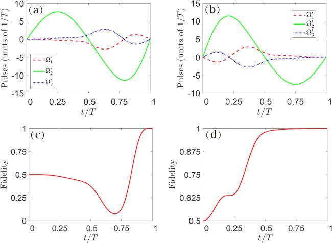
Figure 2. (a) Rabi frequencies ${{\rm{\Omega }}}_{1}^{{\prime} }$, ${{\rm{\Omega }}}_{2}^{{\prime} }$, ${{\rm{\Omega }}}_{3}^{{\prime} }$ (versus t / T) for conversion of the GHZ to KLM state. (b) Rabi frequencies ${{\rm{\Omega }}}_{1}^{{\prime} }$, ${{\rm{\Omega }}}_{2}^{{\prime} }$, ${{\rm{\Omega }}}_{3}^{{\prime} }$ (versus t / T) for conversion of the KLM to GHZ state. (c) The fidelity of the GHZ to KLM state (versus t / T) by simulating the Hamiltonian ( |
4. Numerical simulation and analyses
In this section, we proceed with numerical simulations and analyses. By employing parameters that can be realized experimentally, this study further explores the impact of various decoherence mechanisms on the stability of quantum state evolution. This step aims to verify the effectiveness and robustness of our scheme under realistic experimental conditions.
It is well known that if a unitary transformation is performed from an old picture to a new picture, the quantum state will undergo a phase change. The implementation of the conversion between the GHZ state and KLM state takes place under the new picture as defined by equation (5 ). If discussed in the old picture, a state would experience a phase transformation. Specifically, if a state can be described as ∣ψ⟩ in the new picture, when transformed back to the original picture, it will become ${ \mathcal R }| \psi \rangle $. Although there is a change in phase, once we determine the value of VT, we can derive the specific phase of the final state. What we are concerned with is the probability amplitude of the state. Based on this consideration, we define the fidelity at time t in the new picture as $F=| \langle \psi | {\rho }^{{\prime} }(t)| \psi \rangle | $, where ρ(t) is the density operator in new picture. So, we define the fidelity of obtaining the KLM state from the GHZ state as ${F}_{1}=| \langle {\rm{KLM}}| {\rho }^{{\prime} }(t)| {\rm{KLM}}\rangle | $. Similarly, the fidelity of the GHZ state obtained from the KLM state is ${F}_{2}=| \langle {\rm{GHZ}}| {\rho }^{{\prime} }(t)| {\rm{GHZ}}\rangle | $.
We performed numerical simulations with the Hamiltonian (2 ), the fidelities F1 and F2 are shown in figure 3, where we have chosen the parameter V = 100π/T, which clearly satisfies the $V\gg {\rm{Max}}\{| {{\rm{\Omega }}}_{1}| ,| {{\rm{\Omega }}}_{2}| ,| {{\rm{\Omega }}}_{3}| \}\approx 11.4/T$. Numerical simulation results show that the fidelities are more than 99.7% at the moment of T.
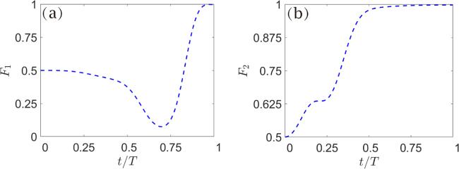
Figure 3. (a) The fidelity F1 versus t / T. (b) The fidelity F2 versus t / T. |
Considering the effects of thermal noise, dephasing, and spontaneous emission on the present scheme, we conducted numerical simulations on the fidelities of interconversions between the GHZ state and KLM state using the master equation [60]
$\begin{eqnarray}\begin{array}{rcl}\dot{\rho } & = & -{\rm{i}}[H(t),\rho ]+{D}_{{\rm{deph}}}(\rho )+{D}_{{\rm{therm}}}(\rho ),\\ {D}_{{\rm{deph}}} & = & \displaystyle \sum _{k=1}^{3}\left[{L}_{k}\rho {L}_{k}^{\dagger }-\frac{1}{2}\left({L}_{k}^{\dagger }{L}_{k}\rho +\rho {L}_{k}^{\dagger }{L}_{k}\right)\right],\\ {D}_{{\rm{therm}}} & = & \displaystyle \sum _{k=4}^{6}\left\{(\bar{n}+1)\left[{L}_{k}\rho {L}_{k}^{\dagger }-\frac{1}{2}\left({L}_{k}^{\dagger }{L}_{k}\rho +\rho {L}_{k}^{\dagger }{L}_{k}\right)\right]\right.\\ & & +\left.\bar{n}\left[{L}_{k}^{\dagger }\rho {L}_{k}-\frac{1}{2}\left({L}_{k}{L}_{k}^{\dagger }\rho +\rho {L}_{k}{L}_{k}^{\dagger }\right)\right]\right\},\end{array}\end{eqnarray}$
where $\bar{n}$ is the average number of thermal phonons which is set in a scope as 0 ∼ 1, when considering the Bose–Einstein distribution, this average phonon number is calculated by $1/({{\rm{e}}}^{\frac{\hslash \omega }{{k}_{B}{ \mathcal T }}}-1)$, which is related to the temperature of the environment ${ \mathcal T }$ and the frequency ω of thermal noise. Lk(k = 1, 2, 3, 4, 5, 6) are the Lindblad operators, which are $\begin{eqnarray}\begin{array}{rcl}{L}_{1} & = & \sqrt{{\gamma }_{1}}\left(| r{\rangle }_{1}{\langle r| -| 0\rangle }_{1}\langle 0| \right),\\ {L}_{2} & = & \sqrt{{\gamma }_{2}}\left(| r{\rangle }_{2}{\langle r| -| 0\rangle }_{2}\langle 0| \right),\\ {L}_{3} & = & \sqrt{{\gamma }_{3}}\left(| r{\rangle }_{3}{\langle r| -| 0\rangle }_{3}\langle 0| \right),\\ {L}_{4} & = & \sqrt{{{\rm{\Gamma }}}_{1}}| 0{\rangle }_{1}\langle r| ,\\ {L}_{5} & = & \sqrt{{{\rm{\Gamma }}}_{2}}| 0{\rangle }_{2}\langle r| ,\\ {L}_{6} & = & \sqrt{{{\rm{\Gamma }}}_{3}}| 0{\rangle }_{3}\langle r| ,\end{array}\end{eqnarray}$
where Γk is atomic spontaneous emission rate from ∣r⟩ to ∣0⟩, γk being the dephasing rate of the kth atom. For simplicity, here we set Γ1 = Γ2 = Γ3 = Γ, γ1 = γ2 = γ3 = γ.In figure 4, we illustrate the effects of atomic spontaneous emission Γ and dephasing rates γ on fidelity (note, Γ, γ unite of 1/T ), where we have set the average number of thermal phonons $\bar{n}=0$. Through figure 4, we can see that this scheme demonstrates robustness against atomic spontaneous emission and dephasing rate.
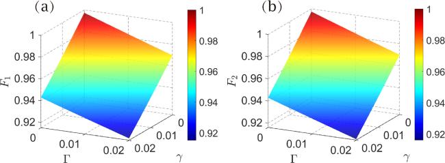
Figure 4. The fidelity (a) F1, (b) F2 versus the decoherence of spontaneous emission Γ and dephasing γ ( Γ, γ unite of 1/T). |
Next, we plotted the fidelity as it varies with atomic spontaneous emission and the average number of thermal photons as shown in figure 5, even when $\bar{n}=1$ and Γ = 0.02 (unites of 1/T), the fidelity remains above 91.5%. Therefore, we can prove that the scheme is robust against spontaneous emission and thermal noise. Here, we consider the total evolutionary time T = 20 μs, which is still much less than the reported coherence time of the Rydberg atom. By considering a group of parameters that are feasible for experiments, Γ = 1 kHz, γ = 1 kHz (i.e. 0.02 unites of 1/T) and an experimental temperature of 20 μK [61], assuming the frequency of thermal noise as ω = 2π × 1 MHz (i.e. $\bar{n}\sim 0.1$ ). We can obtain F1 = 91.16% and F2 = 91.17%. This indicates the scheme demonstrates robustness against decoherence.
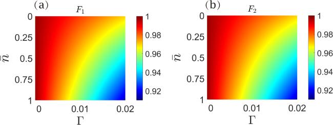
Figure 5. The fidelity (a) F1, (b) F2 versus the spontaneous emission Γ and and the average number of thermal phonons $\bar{n}$. |
In order to further explore the robustness of the protocol under realistic experimental conditions, we will next introduce a factor that is closer to the actual situation, i.e. Gaussian white noise. This noise model will be applied to the control field to simulate the unavoidable environmental disturbances and systematic errors in the experiment. By introducing Gaussian white noise into our control scheme, we evaluate the effect of noise on system evolution and final state fidelities. Then additive white Gaussian noise (AWGN) leads to the noisy control field as
$\begin{eqnarray}{{\rm{\Omega }}}_{k}^{{\rm{n}}{\rm{o}}}={{\rm{\Omega }}}_{k}+{\rm{Awgn}}\left({{\rm{\Omega }}}_{k},\kappa \right),\end{eqnarray}$
where ${\rm{Awgn}}\left({{\rm{\Omega }}}_{k},\kappa \right)$ denotes a function-generating AWGN with signal-to-noise ratio (SNR) κ for Ωk. We performed ten separate simulations for each different SNR, the results are shown in the figure 6. We can see that even with SNR κ = 10, the fidelities are still above 97%. Therefore, this scheme is robust to Gaussian white noise.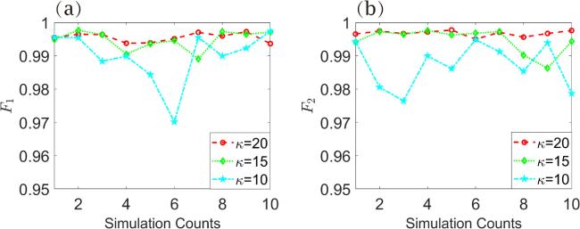
Figure 6. (a) The fidelity F1 of the conversion from GHZ to KLM state under AWGN versus run number. (b) The fidelity F2 of the conversion from KLM to GHZ state under AWGN versus run number. |
5. Summary
In summary, we have proposed a scheme to realize the interconversion of the GHZ and KLM state of atomic system. We simplify the dynamics by utilizing the energy level shift terms of the Rydberg atomic system, the effective Hamiltonian for the physical model can ultimately be simplified to a four-level Hamiltonian with basis {∣000⟩, ∣r00⟩, ∣rr0⟩, ∣rrr⟩}. In this evolutionary space, we implement the interconversion of the GHZ and KLM state by Lie-transform-based pulse design. We performed numerical simulations to evaluate the influence of various decoherence factors, such as thermal noise, dephasing and spontaneous emission, the numerical simulation results show that the scheme is robust against various decoherence. In addition, we analyze the effect of Gaussian noise and mismatch of detuning on the results. In a nutshell, this scheme features deterministic and reversible state conversions, and has high fidelities in both directions. We believe this paper will offer fresh insights and potentially introduce new ideas, contributing to the advancement of quantum information exploration.