


1. Introduction
2. Classification of fully entangled states
2.1. Entanglement quantifiers and detectors
2.2. Classification tree
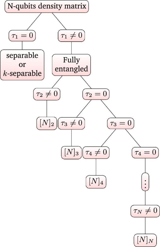
Figure 1. Classification of entanglement for N-qubit states. |
2.3. Types of entanglement in symmetric systems
N-entanglement, where performing a partial trace over any individual subsystem yields a separable state. This type of entanglement is genuinely shared among all N parties.
(N − 1)-entanglement, which disappears when tracing out any two individual subsystems. This entanglement is shared among (N − 1)-tuples.
The 2-entanglement, being the most resilient against partial trace operations, as persists even when traced out over any (N − 2) subsystems. Here, entanglement is shared among all possible pairs.
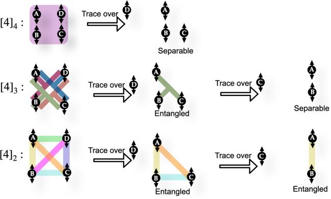
Figure 2. The fragility of the entanglement in each class over the partial trace. |
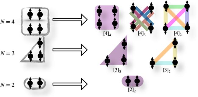
Figure 3. Entanglement classes in symmetric fully entangled states for four, three, and two qubits partitions. |
3. Classification using machine learning
3.1. Machine learning, deep learning and artificial neural networks
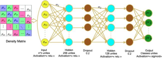
Figure 4. The adopted architecture of the Neural Network. |
3.2. Data set
1. Generate a random density matrix state ρ of 2 qubits.
2. Compute the concurrence of ρ. If it is equal to 0 we save ρ in our data set as 'Separable', else we save it as 'Entangled'.
1. Generate a random density matrix state ρ according to the number of qubits In our application we use 3-qubits and 4-qubits systems.
2. Compute the different i-tangles and assign the corresponding class according to the classification established in section
For 3 qubits, if τ1 = 0, we save ρ in our data set as 'separable', else if τ2 ≠ 0, we save it in our data set as '[3]2', else we save it as '[3]3'.
For 4 qubits, if τ1 = 0, we save ρ in our data set as 'separable', else if τ2 ≠ 0, we save it in our data set as '[4]2', else if τ3 ≠ 0 we save it as '[4]3', else we save it as '[4]4'.
for 2-qubit systems, we generated 400 000 density matrices, 200 000 pure and 200 000 mixed, each type containing 100 000 of each class separable/entangled.
for 3-qubit systems, we generated 60 000 density matrices, 30 000 pure and 30 000 mixed, each type containing 10 000 of each class k-separable or separable /[3]2/[3]3.
for 4-qubit systems, we generated 80 000 density matrices, 40 000 pure and 40 000 mixed, each type containing 10 000 of each class k-separable or separable /[4]2/[4]3/[4]4.
3.3. Results
1. Accuracy, is the proportion of the total number of correct predictions:
2. Precision, is a measure of the number of cases in which a specific class i has been correctly predicted:
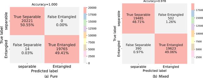
Figure 5. The testing confusion matrix for the classification of pure (a) and mixed (b) bipartite density matrices. |
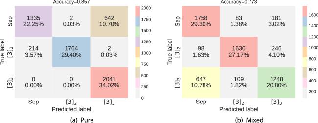
Figure 6. The testing confusion matrix for the classification of pure (a) and mixed (b) tripartite density matrices. |
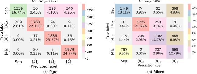
Figure 7. The testing confusion matrix for the classification of pure (a) and mixed (b) four-partite density matrices. |
Table 1. Verification of the classification of some well-known pure states. |
| Verification of pure states | |||
|---|---|---|---|
| Dim | State | True class | Predict class |
| 2 qubits | $| {\psi }_{1}\rangle =\frac{1}{\sqrt{2}}(| 00\rangle +| 11\rangle )$ | Ent | Ent ✓ |
| $| {\psi }_{2}\rangle =\frac{1}{\sqrt{2}}(| 01\rangle +| 10\rangle )$ | Ent | Ent ✓ | |
| $| {\psi }_{3}\rangle =\frac{1}{\sqrt{2}}(| 00\rangle -| 11\rangle )$ | Ent | Ent ✓ | |
| $| {\psi }_{4}\rangle =\frac{1}{\sqrt{2}}(| 01\rangle -| 10\rangle )$ | Ent | Ent ✓ | |
| $| {\psi }_{5}\rangle =\frac{1}{\sqrt{2}}(| 00\rangle +| 01\rangle )$ | Sep | Sep ✓ | |
| $| {\psi }_{6}\rangle =\frac{1}{\sqrt{2}}(| 10\rangle +| 11\rangle )$ | Sep | sep ✓ | |
| $| {\psi }_{7}\rangle =\frac{1}{2}(| 00\rangle +| 01\rangle +| 10\rangle +| 11\rangle )$ | Sep | Sep ✓ | |
| | |||
| 3 qubits | $| {\phi }_{1}\rangle =\frac{1}{\sqrt{2}}(| 000\rangle +| 111\rangle )$ | [3]3 | [3]3✓ |
| $| {\phi }_{2}\rangle =\frac{1}{\sqrt{3}}(| 001\rangle +| 010\rangle +| 100\rangle )$ | [3]2 | [3]2✓ | |
| $| {\phi }_{3}\rangle =\frac{1}{\sqrt{3}}(| 110\rangle +| 101\rangle +| 011\rangle )$ | [3]2 | [3]2✓ | |
| $| {\phi }_{4}\rangle =\frac{1}{\sqrt{3}}(| 010\rangle +| 001\rangle +| 011\rangle )$ | K-Sep | Sep ✓ | |
| $| {\phi }_{5}\rangle =\frac{1}{\sqrt{2}}(| 000\rangle +| 001\rangle )$ | Sep | [3]3 ✗ | |
| | |||
| 4 qubits | $| {\chi }_{1}\rangle =\frac{1}{\sqrt{2}}(| 0000\rangle +| 1111\rangle )$ | [4]4 | [4]4✓ |
| $| {\chi }_{2}\rangle =\frac{1}{2}(| 0001\rangle +| 0010\rangle +| 0100\rangle +| 1000\rangle )$ | [4]2 | [4]2✓ | |
| $| {\chi }_{3}\rangle =\frac{1}{2}(| 1110\rangle +| 1101\rangle +| 1011\rangle +| 0111\rangle )$ | [4]2 | Sep ✗ | |
| $| {\chi }_{4}\rangle =\frac{1}{\sqrt{5}}(| 0000\rangle +| 0111\rangle +| 1011\rangle +| 1101\rangle +| 1110\rangle )$ | [4]3 | [4]3✓ | |
| $| {\chi }_{5}\rangle =\frac{1}{\sqrt{5}}(| 1000\rangle +| 0100\rangle +| 0010\rangle +| 0001\rangle +| 1111\rangle )$ | [4]3 | [4]3✓ | |
| $| {\chi }_{6}\rangle =\frac{1}{2}(| 0000\rangle +| 0011\rangle +| 0010\rangle +| 0001\rangle )$ | K-Sep | Sep ✓ | |
Table 2. Verification of the classification of some mixture of the states used in table 1. |
| Verification of mixed states | |||
|---|---|---|---|
| Dim | State | True class | Predict class |
| 2 qubits | ρ1 = 0.5(∣ψ1⟩⟨ψ1∣) + 0.5(∣ψ3⟩⟨ψ3∣) | Sep | Sep ✓ |
| ρ2 = 0.8(∣ψ1⟩⟨ψ1∣) + 0.2(∣ψ3⟩⟨ψ3∣) | Ent | Ent ✓ | |
| ρ3 = 0.5(∣ψ2⟩⟨ψ2∣) + 0.5(∣ψ6⟩⟨ψ6∣) | Sep | Sep ✓ | |
| ρ4 = 0.8(∣ψ2⟩⟨ψ2∣) + 0.2(∣ψ6⟩⟨ψ6∣) | Ent | Ent ✓ | |
| | |||
| 3 qubits | σ1 = 0.8(∣φ1⟩⟨φ1∣) + 0.2(∣φ3⟩⟨φ3∣) | [3]3 | [3]3✓ |
| σ2 = 0.8(∣φ1⟩⟨φ1∣) + 0.2(∣φ3⟩⟨φ3∣) | [3]3 | [3]3✓ | |
| σ3 = 0.8(∣φ1⟩⟨φ1∣) + 0.2(∣φ3⟩⟨φ3∣) | [3]3 | [3]3✓ | |
| σ4 = 0.8(∣φ1⟩⟨φ1∣) + 0.2(∣φ3⟩⟨φ3∣) | [3]3 | Sep ✗ | |
| | |||
| 4 qubits | μ1 = 0.5(∣χ1⟩⟨χ1∣) + 0.5(∣χ3⟩⟨χ3∣) | [4]4 | [4]4✓ |
| μ2 = 0.2(∣χ2⟩⟨χ2∣) + 0.8(∣χ4⟩⟨χ4∣) | [4]3 | [4]3✓ | |
| μ3 = 0.8(∣χ6⟩⟨χ6∣) + 0.2(∣χ5⟩⟨χ5∣) | Sep | Sep ✓ | |
| μ4 = 0.8(∣χ1⟩⟨χ1∣) + 0.2(∣χ3⟩⟨χ3∣) | [4]4 | Sep ✗ | |
| μ5 = 0.8(∣χ5⟩⟨χ5∣) + 0.2(∣χ2⟩⟨χ2∣) | [4]3 | [4]4 ✗ | |