


1. Introduction
Quantum sensing as an important quantum technology has attracted widespread interest in recent years, following the pioneering works of Helstrom [1–3] and Holevo [4]. The key idea is to utilize non-classical features [5] of the quantum probes to improve the sensing precision beyond its classical counterpart [6]. The classical sensing scheme uses N repeated measurements to improve the sensing precision by a factor $\sqrt{N}$ according to the central limit theorem. In quantum sensing, using N non-interacting quantum probes prepared in certain entangled states allows the sensing precision to attain the Heisenberg scaling 1/N [7–9] in the noise-free case. In practice, however, the decoherence induced by environmental noises limits the utility of N-probe entanglement and hence degrades the sensing precision dramatically [10–15]. Experimentally, the advantage of quantum sensing has been demonstrated in a variety of quantum platforms (see [16, 17] for a review), including optical systems [18–22], atomic systems [23, 24], superconducting circuits [10], and nuclear magnetic resonance systems [25]. Theoretically, exploring the quantum advantages [25] of various quantum sensors in noisy environments has been a central subject over recent years [26–39] (see [40–42] for a review).
At present, two-level systems (hereafter referred to as spin-1/2's) are one of the prevalent quantum sensors. For N spin-1/2's, three important states have been widely utilized for frequency estimation: the spin coherent state (SC), the Schrödinger cat state or Greenberger–Horne–Zeilinger state (GHZ) [7, 8], and the maximal spin squeezed state [43, 44] (SS). In the noiseless case, GHZ and SS give the best sensing precision δωGHZ = δωSS = 1/N following the Heisenberg scaling. This outperforms the classical scaling $\delta {\omega }_{{\rm{SC}}}=1/\sqrt{N}$ of SC, which is equivalent to N repeated measurements with one spin-1/2. In the presence of noises, the most detrimental decoherence for frequency estimation is dephasing, because it attenuates the off-diagonal coherence that stores the information about the frequency to be estimated. There are two kinds of dephasing: (i) Individual (or local) dephasing due to coupling of each spin-1/2 to an independent noise; (ii) Collective (or global) dephasing due to coupling of all spin-1/2's to the same noise. The precision of GHZ under individual dephasing has been studied by many works based on different noise models [12, 26, 27, 32, 33, 37, 39, 44, 45]. The precision of SS under individual dephasing by Markovian noises has also been established [44]. However, the precision of SS under individual dephasing by non-Markovian noises and, more importantly, the precision of GHZ, SS, and SC under collective dephasing remain unexplored.
Here we provide the missing information through a systematic study of the sensing precision of GHZ, SS, and SC under either individual or collective dephasing due to general Gaussian noise, going from the Markovian limit to the extreme non-Markovian limit. Our central results are summarized in table 1, where the precision of GHZ, SS, and SC are relative values compared to the precision δωcl of the classical scheme of N repeated measurements with one spin-1/2 (e.g., GHZ listed in table 1 is actually δωGHZ/δωcl):
$\begin{eqnarray*}\delta {\omega }_{{\rm{cl}}}\equiv \left\{\begin{array}{ll}\sqrt{2{\rm{e}}\alpha /N} & \,\rm{(Markovian\, noise)}\,\\ {(4{\rm{e}}\alpha )}^{1/4}/\sqrt{N} & \,\rm{(non-Markovian\, noise)}\,\end{array}\right.,\end{eqnarray*}$
and the parameter α characterizes the noise-induced decay of the total spin of all the N spin-1/2's. For individual dephasing, table 1 agrees with existing works, e.g., GHZ and SC provide no improvement over the classical scheme [45] and $\delta {\omega }_{{\rm{SS}}}/\delta {\omega }_{{\rm{SC}}}=1/\sqrt{{\rm{e}}}$ [44] under Markovian noise, and δωGHZ/δωcl ∝ 1/N1/4 under non-Markovian noise [12, 26]. For N ≫ 1, table 1 reveals two surprises. First, SC is worse than the classical scheme under collective dephasing, despite its equivalence to the classical scheme under individual dephasing. Second, SS give the best precision in all cases, with a constant factor improvement (Markovian noise) or a scaling improvement (non-Markovian noise) over the classical scheme. By contrast, the widely studied GHZ outperforms the classical scheme only under individual dephasing by non-Markovian noises. These results establish the quantum advantage of SS for noisy frequency estimation based on two classes of quantum sensors: (1) A collection of spin-1/2's, which may suffer from both individual dephasing and collective dephasing. (2) Naturally occurring high-spin particles (such as the excited state of rhenium nucleus with spin quantum number S = 8, astatine nucleus with S = 39/2 or S = 41/2 [46], and the atoms or molecules in magnetic materials [47, 48]), which only suffer from collective dephasing. Therefore, our results are relevant to many quantum sensing platforms [10, 23–25].Table 1. Sensing precision (relative to the classical scheme of N repeated measurement with one spin-1/2) for noisy frequency estimation using N spin-1/2's prepared in three initial states: the cat state (GHZ), the maximal spin squeezed state (SS), and the spin coherent state (SC). Under individual dephasing, the result for SS is valid only when N ≫ 1. Under collective dephasing, the results for SS and SC are valid only when N ≫ 1. |
| Individual dephasing | GHZ | SS | SC |
| Markovian noise | 1 | $1/\sqrt{{\rm{e}}}$ | 1 |
| Non-Markovian noise | 1/N1/4 | [2/(eN)]1/4 | 1 |
| | |||
| Collective dephasing | GHZ | SS | SC |
| Markovian noise | $\sqrt{N}$ | $\,\sqrt{2/{\rm{e}}}$ | $\sqrt{N/{\rm{e}}}$ |
| Non-Markovian noise | 1 | [4/(eN)]1/4 | (2N/e)1/4 |
2. Procedures for quantum sensing
The typical procedures for estimating an unknown real parameter λ using a quantum probe consists of three steps [49]:
(1) The quantum probe is prepared into certain initial state ρ and then undergoes certain λ-dependent evolution into a final state ρλ parametrized by the parameter λ to be estimated;
(2) The quantum probe undergoes a general measurement described by a set of positive operators {Πx} satisfying ∑xΠx = 1. The measurement outcome x is a random variable sampled from the probability distribution ${P}_{\lambda }\left(x\right)={\rm{Tr}}{{\rm{\Pi }}}_{x}{\rho }_{\lambda }$ that depends on λ [50]. Repeating the initialization-evolution-measurement cycle ν times yields ν independent data x ≡ (x1, ⋯ , xν), whose distribution is the direct product of the distribution of each datum: Pλ(x) = Pλ(x1) ⋯ Pλ(xν).
(3) Given x = (x1, ⋯ , xν), an unbiased estimator $\hat{\lambda }\left({\boldsymbol{x}}\right)$ to λ is constructed. Here $\hat{\lambda }\left({\boldsymbol{x}}\right)$ is a real-valued function of x, hence is also a random variable. With E[⋯ ] ≡ ∑x(⋯ )Pλ(x), the unbiased condition reads $\lambda ={\boldsymbol{E}}[\hat{\lambda }\left({\boldsymbol{x}}\right)]$ and the sensing precision/error $\delta \hat{\lambda }\equiv \sqrt{{\rm{var}}(\hat{\lambda })}$ is defined as the square root of the variance ${\rm{var}}(\hat{\lambda })\equiv {\boldsymbol{E}}[{\hat{\lambda }}^{2}]-{({\boldsymbol{E}}[\hat{\lambda }])}^{2}$ of $\hat{\lambda }$.
The estimation precision of any unbiased estimator $\hat{\lambda }({\boldsymbol{x}})$ based on ν repeated measurement outcomes x ≡ (x1, ⋯ , xν) sampled from ${P}_{\lambda }\left({\boldsymbol{x}}\right)$ obeys the Cramér–Rao bound $\delta \hat{\lambda }\geqslant 1/\sqrt{\nu F}$ [51], where $F\equiv {\boldsymbol{E}}[{L}_{\lambda }^{2}(x)]$ is the (classical) Fisher information (CFI) from one datum x and ${L}_{\lambda }(x)\equiv \partial \mathrm{ln}{P}_{\lambda }\left(x\right)/\partial \lambda $ is the (classical) score of the distribution Pλ(x). The quantum analog to the classical score Lλ(x) is the quantum score Lλ, a Hermitian operator satisfying ${\partial }_{\lambda }{\rho }_{\lambda }=\left({L}_{\lambda }{\rho }_{\lambda }+{\rho }_{\lambda }{L}_{\lambda }\right)/2$ [52]. The CFI F associated with the distribution Pλ(x) of any measurement {Πx} performed on ρλ is upper bounded by the quantum Fisher information (QFI) ${ \mathcal F }\equiv {\rm{Tr}}{\rho }_{\lambda }{L}_{\lambda }^{2}$ [52]. This leads to the quantum Cramér–Rao bound:
$\begin{eqnarray*}\delta \hat{\lambda }\geqslant \frac{1}{\sqrt{\nu F}}\geqslant \frac{1}{\sqrt{\nu { \mathcal F }}}.\end{eqnarray*}$
In this work, we focus on estimating the small deviation of λ from a known value λ0. In this case, both inequalities can be saturated simultaneously, i.e., there exists an optimal measurement making $F={ \mathcal F }$ (such as the projective measurement over the quantum score ${L}_{{\lambda }_{0}}$, see [53] and references therein) and there exists an efficient unbiased estimator $\hat{\lambda }$ with precision $\delta \hat{\lambda }=1/\sqrt{\nu F}=1/\sqrt{\nu { \mathcal F }}$. Therefore, the QFI determines the ultimate achievable estimation precision $\delta {\hat{\lambda }}_{\min }=1/\sqrt{\nu { \mathcal F }}$.
In cases where the quantum state ρλ or its QFI is difficult to calculate, we may resort to the inversion estimator ${\hat{\lambda }}_{{\rm{inv}}}({\boldsymbol{x}})$ based on ν repeated measurement outcomes x = (x1, ⋯ , xν) of some observable O (a Hermitian operator). The idea is that the sample average $\bar{x}\equiv ({x}_{1}+\cdots +{x}_{\nu })/\nu $ should be close to the statistical mean value ${\langle O\rangle }_{\lambda }\equiv {\rm{Tr}}{\rho }_{\lambda }O\equiv f(\lambda )$, so that λ should be close to ${f}^{-1}(\bar{x})$. This identifies the inversion estimator ${\hat{\lambda }}_{{\rm{inv}}}({\boldsymbol{x}})={f}^{-1}(\bar{x})$, whose precision is determined by the average value ⟨O⟩λ and root-mean-square fluctuation ${(\delta O)}_{\lambda }\equiv {({\langle {O}^{2}\rangle }_{\lambda }-{\langle O\rangle }_{\lambda }^{2})}^{1/2}$ of the observable through the error propagation formula [54]
$\begin{eqnarray*}\delta {\hat{\lambda }}_{{\rm{inv}}}=\frac{{(\delta O)}_{\lambda }}{\sqrt{\nu }\left|{\partial }_{\lambda }{\langle O\rangle }_{\lambda }\right|}.\end{eqnarray*}$
3. Spin-S for noisy frequency estimation
Here we consider estimating the Larmor precession frequency ω of a spin-S (S = 1/2, 1, 3/2, ⋯ ) in the presence of a general Gaussian dephasing noise. The spin-S may be either a naturally occurring particle or be formed by adding the angular momentum of N = 2S spatially separated spin-1/2's: S = s1 + s2 + ⋯ + sN. From now on, we define N ≡ 2S and use N to quantify the quantum resources. The collective dephasing of the spin-S is described by the Hamiltonian [49]
$\begin{eqnarray}H(t)=\left[\omega +\tilde{\omega }(t)\right]{S}_{z},\end{eqnarray}$
where $\tilde{\omega }(t)$ is a Gaussian noise characterized by the auto-correlation function $C(\tau )=\overline{\tilde{\omega }(\tau )\tilde{\omega }(0)}$ (the overbar denotes the average over the noise distribution), an even function of τ. When the spin-S is formed by N spin-1/2's, the term $\tilde{\omega }(t){S}_{z}={\sum }_{i}\tilde{\omega }(t){s}_{i,z}$ describes the coupling of all these spin-1/2's to a common noise $\tilde{\omega }(t)$, hence the name 'collective dephasing'. The spin-S formed by N spin-1/2's may also suffer from individual dephasing due to the coupling of each spin-1/2's to an independent noise: $\begin{eqnarray}H(t)=\omega {S}_{z}+{\sum }_{i}{\tilde{\omega }}_{i}(t){s}_{i,z},\end{eqnarray}$
where ${\tilde{\omega }}_{1}(t),\cdots \,,{\tilde{\omega }}_{N}(t)$ are identically distributed and statistically independent Gaussian noises characterized by the same auto-correlation function $C(\tau )=\overline{{\tilde{\omega }}_{i}(\tau ){\tilde{\omega }}_{i}(0)}$ as $\tilde{\omega }(t)$. Next we begin with the noiseless case and then take into account the noise. For both cases, we consider three kinds of initial states (⟨ ⋯ ⟩ denotes the average in the initial state):(1) GHZ, i.e., an equal superposition of the extremal eigenstates ∣ ± S⟩ of Sz with eigenvalues ± S [7, 8, 10, 53]:
$\begin{eqnarray}\left|{\psi }_{{\rm{GHZ}}}\right\rangle \equiv \frac{1}{\sqrt{2}}\left(\left|S\right\rangle +\left|-S\right\rangle \right)=\frac{1}{\sqrt{2}}\left(| \uparrow {\rangle }^{\otimes N}+| \downarrow {\rangle }^{\otimes N}\right),\end{eqnarray}$
where the second expression is valid when the spin-S is formed by N spin-1/2's: $\left|S\right\rangle =| \uparrow {\rangle }^{\otimes N}$ and $\left|-S\right\rangle =| \downarrow {\rangle }^{\otimes N}$.(2) SC
$\begin{eqnarray*}| {\psi }_{{\rm{SC}}}\rangle \equiv {{\rm{e}}}^{-{\rm{i}}(\pi /2){S}_{y}}| S\rangle ={\left(\frac{| \uparrow \rangle +| \downarrow \rangle }{\sqrt{2}}\right)}^{\otimes N},\end{eqnarray*}$
where the second expression is valid when the spin-S is formed by N spin-1/2's: ${{\rm{e}}}^{-{\rm{i}}(\pi /2){S}_{y}}| S\rangle ={({{\rm{e}}}^{-{\rm{i}}(\pi /2){s}_{y}}| \uparrow \rangle )}^{\otimes N}$. This SC has maximal average spin ⟨S⟩ = Sex along the x axis and isotropic transverse fluctuations $\delta {S}_{y}=\delta {S}_{z}=\sqrt{S/2}$, where $\delta O\equiv {(\langle {O}^{2}\rangle -{\langle O\rangle }^{2})}^{1/2}$. The average spin ⟨Sx⟩ = S and the transverse fluctuations δSy, δSz saturate the Heisenberg uncertainty relation $\delta {S}_{y}\delta {S}_{z}\geqslant \left|\langle {S}_{x}\rangle \right|/2=S/2$.(3) SS ∣ψSS⟩ [43, 55] with the same maximal average spin ⟨S⟩ = Sex as the spin coherent state, minimal transverse fluctuation δSy = 1/2 along the y axis, and maximal transverse fluctuation δSz = S along the z axis. The average spin ⟨Sx⟩ = S and the transverse fluctuations δSy, δSz saturate the Heisenberg uncertainty relation $\delta {S}_{y}\delta {S}_{z}\geqslant \left|\langle {S}_{x}\rangle \right|/2=S/2$.
In the noiseless case, for a general pure initial state ∣ψ⟩, the final state $| \psi (t)\rangle ={{\rm{e}}}^{-{\rm{i}}\omega t{S}_{z}}| \psi \rangle $ after an interval t carries the QFI ${ \mathcal F }(t)=4{t}^{2}{(\delta {S}_{z})}^{2}$ about the unknown parameter ω, where ${(\delta {S}_{z})}^{2}=\langle {S}_{z}^{2}\rangle -{\langle {S}_{z}\rangle }^{2}$ is the fluctuation in the initial state ∣ψ⟩. Therefore, GHZ and SS are both optimal, because they both give maximal ${(\delta {S}_{z})}^{2}={S}^{2}={(N/2)}^{2}$, hence the best sensing precision after ν repeated measurements
$\begin{eqnarray}\delta {\omega }_{{\rm{GHZ}}}=\delta {\omega }_{{\rm{SS}}}=\frac{1}{\sqrt{\nu }}\frac{1}{Nt},\end{eqnarray}$
following the Heisenberg scaling 1/N. When the initial state is SC with $\delta {S}_{z}^{2}=S/2=N/4$, the final-state QFI is ${{ \mathcal F }}_{{\rm{SC}}}(t)=N{t}^{2}$ and the sensing precision after ν repeated measurements is $\begin{eqnarray}\delta {\omega }_{{\rm{SC}}}=\frac{1}{\sqrt{\nu }}\frac{1}{\sqrt{N}t},\end{eqnarray}$
which follows the classical scaling $1/\sqrt{N}$. Intuitively, starting from the SC, each spin-1/2 evolves independently: $\begin{eqnarray*}{{\rm{e}}}^{-{\rm{i}}\omega t{S}_{z}}| {\psi }_{{\rm{SC}}}\rangle ={\left({{\rm{e}}}^{-{\rm{i}}\omega t{s}_{z}}\frac{| \uparrow \rangle +| \downarrow \rangle }{\sqrt{2}}\right)}^{\otimes N},\end{eqnarray*}$
thus using SC as the initial state is equivalent to the classical scheme of N repeated measurements with one spin-1/2. Even in the presence of individual dephasing, this physical picture remains valid.3.1. General Gaussian dephasing noise
In the presence of a general Gaussian dephasing noise, the evolution becomes non-unitary. Since most cases of the individual dephasing have been discussed in the literature [12, 27, 32, 33, 39, 44, 45], we focus on collective dephasing and only list the final results for individual dephasing, leaving the detailed derivations in the Appendix. Under collective dephasing, a pure initial state ∣ψ⟩ evolves to a mixed state after an interval t:
$\begin{eqnarray*}\rho (t)=\overline{| \psi (t)\rangle \langle \psi (t)| },\end{eqnarray*}$
where $| \psi (t)\rangle ={{\rm{e}}}^{-{\rm{i}}\omega t{S}_{z}}{{\rm{e}}}^{-{\rm{i}}\tilde{\varphi }(t){S}_{z}}| \psi \rangle $ contains a random phase $\tilde{\varphi }(t)\equiv {\int }_{0}^{t}\tilde{\omega }({t}^{{\prime} }){\rm{d}}{t}^{{\prime} }$ due to the noise and $\overline{(\cdots \,)}$ stands for the average over the distribution of the noise. For a general initial state, the final-state QFI is difficult to calculate, thus finding the optimal initial state is challenging. Here instead of searching for the optimal initial state, we consider three representative initial states: GHZ, SS, and SC.When the initial state is GHZ, the final state is A ) 4 ) and (5 ), respectively. For S = 1/2, hence N = 1, all initial states coincide and give the same precision. In all cases, the quantity χ(t) completely determines the influence of the noise on the frequency estimation. Physically, χ(t) is the decay exponent of the average spin vector in the xy plane: $| {\langle {S}_{+}\rangle }_{t}/{\langle {S}_{+}\rangle }_{t=0}| ={{\rm{e}}}^{-\chi (t)}$ (see appendix A ).
$\begin{eqnarray*}\begin{array}{rcl}\rho \left(t\right) & = & \displaystyle \frac{1}{2}\left(\left|S\right\rangle \left\langle S\right|\right.\\ & & \left.+\left|-S\right\rangle \left\langle -S\right|\right)+\displaystyle \frac{1}{2}{{\rm{e}}}^{-{N}^{2}\chi (t)}\left({{\rm{e}}}^{-{\rm{i}}N\omega t}\left|S\right\rangle \left\langle -S\right|+h.c.\right),\end{array}\end{eqnarray*}$
where $\begin{eqnarray}\chi (t)\equiv \frac{1}{2}\overline{{\tilde{\varphi }}^{2}(t)}={\int }_{0}^{t}{\rm{d}}\tau \,(t-\tau )C(\tau )\end{eqnarray}$
accounts for the noise-induced decoherence. The QFI of the final state $\rho \left(t\right)$ is ${{ \mathcal F }}_{{\rm{GHZ}}}(t)={N}^{2}{t}^{2}{{\rm{e}}}^{-2{N}^{2}\chi (t)}$ and the ultimate sensing precision is $\begin{eqnarray*}\delta {\omega }_{{\rm{GHZ}}}=\frac{1}{\sqrt{\nu {{ \mathcal F }}_{{\rm{GHZ}}}(t)}}=\frac{1}{\sqrt{\nu }Nt{{\rm{e}}}^{-{N}^{2}\chi (t)}}.\end{eqnarray*}$
When the initial state is SS or SC, the final-state QFI is difficult to calculate analytically. Thus we resort to the inversion estimator based on measuring the spin S along certain axis. After optimizing the measurement axis, the sensing precision of the inversion estimator based on ν repeated measurements is (see appendix $\begin{eqnarray*}\begin{array}{rcl}\delta {\omega }_{{\rm{SS}}} & = & \frac{\sqrt{{{\rm{e}}}^{-2\chi (t)}/N+\left({{\rm{e}}}^{2\chi (t)}-{{\rm{e}}}^{-2\chi (t)}\right)}}{\sqrt{\nu N}t},\\ \delta {\omega }_{{\rm{SC}}} & = & \frac{\sqrt{{{\rm{e}}}^{-2\chi (t)}+\frac{1}{2}\left(N+1\right)\left({{\rm{e}}}^{2\chi (t)}-{{\rm{e}}}^{-2\chi (t)}\right)}}{\sqrt{\nu N}t}.\end{array}\end{eqnarray*}$
In the noiseless case χ(t) = 0, they reduce to equations (In the above, we have considered using GHZ, SS, and SC as initial states to estimate the Larmor precession frequency ω from ν repeated measurements of duration t, with a total time cost T = νt. For fixed N and fixed T = νt (assumed to be sufficiently large), the best sensing precision is obtained by optimizing t:
$\begin{eqnarray*}\begin{array}{rcl}\delta {\omega }_{{\rm{GHZ}}}\sqrt{T} & = & \mathop{\min }\limits_{t\in [0,T]}\frac{1}{N\sqrt{t}{{\rm{e}}}^{-{N}^{2}\chi (t)}},\\ \delta {\omega }_{{\rm{SS}}}\sqrt{T} & = & \mathop{\min }\limits_{t\in [0,T]}\frac{\sqrt{{{\rm{e}}}^{-2\chi (t)}/N+\left({{\rm{e}}}^{2\chi (t)}-{{\rm{e}}}^{-2\chi (t)}\right)}}{\sqrt{Nt}},\\ \delta {\omega }_{{\rm{SC}}}\sqrt{T} & = & \mathop{\min }\limits_{t\in [0,T]}\frac{\sqrt{{{\rm{e}}}^{-2\chi (t)}+\frac{1}{2}\left(N+1\right)\left({{\rm{e}}}^{2\chi (t)}-{{\rm{e}}}^{-2\chi (t)}\right)}}{\sqrt{Nt}}.\end{array}\end{eqnarray*}$
Inspection immediately shows δωSS ≤ δωSC and, when N ≫ 1, $\delta {\omega }_{{\rm{SC}}}\,\geqslant \,\sqrt{N/2}\delta {\omega }_{{\rm{SS}}}$. The behavior of δωGHZ, δωSS, and δωSC depends crucially on the decoherence exponent χ(t) ≥ 0, which in turn is determined by the details of the noise starting from χ(0) = 0.Next we fix T and discuss the scaling about N. To enable an analytical discussion, we assume χ(t) = αtβ (see the next subsection for justification), where α > 0 and β = 1, 2, ⋯ are determined by the details of the noise. The best sensing precision and the optimal evolution time for each initial state are listed in tables 2 and 3, respectively (the derivations for individual dephasing are given in appendix B ).
Table 2. Frequency estimation precision using the cat state (GHZ), maximal spin squeezed state (SS), and spin coherent state (SC) as initial states, given the decay exponent χ(t) = αtβ of the average spin vector in the xy plane. The special case β = 1 is obtained by taking the limit β → 1, so that (β − 1)1−1/β → 1. For collective dephasing, the results for SS and SC are valid only when N ≫ 1. For individual dephasing, the results for SS are valid only when N ≫ 1. |
| $\delta {\omega }_{{\rm{GHZ}}}\sqrt{T}$ | $\delta {\omega }_{{\rm{SS}}}\sqrt{T}$ | $\delta {\omega }_{{\rm{SC}}}\sqrt{T}$ | |
|---|---|---|---|
| Collective dephasing | $\frac{{(2{\rm{e}}\alpha \beta )}^{1/(2\beta )}}{{N}^{1-1/\beta }}$ | $\sqrt{\frac{{(4\alpha )}^{1/\beta }\beta }{{(\beta -1)}^{1-1/\beta }}}\frac{1}{{N}^{1-1/(2\beta )}}$ | $\sqrt{\frac{{(2\alpha )}^{1/\beta }\beta }{{(\beta -1)}^{1-1/\beta }}}\frac{1}{\sqrt{{N}^{1-1/\beta }}}$ |
| β = 1 | $\sqrt{2{\rm{e}}\alpha }$ | $2\sqrt{\alpha /N}$ | $\sqrt{2\alpha }$ |
| β = 2 | $\frac{{(4{\rm{e}}\alpha )}^{1/4}}{\sqrt{N}}$ | $\frac{2{\alpha }^{1/4}}{{N}^{3/4}}$ | $\frac{{2}^{3/4}{\alpha }^{1/4}}{{N}^{1/4}}$ |
| | |||
| Individual dephasing | $\frac{{(2{\rm{e}}\alpha \beta )}^{1/(2\beta )}}{{N}^{1-1/(2\beta )}}$ | $\sqrt{\frac{{(2\alpha )}^{1/\beta }\beta }{{(\beta -1)}^{1-1/\beta }}}\frac{1}{{N}^{1-1/(2\beta )}}$ | $\,\,\frac{{(2{\rm{e}}\alpha \beta )}^{1/(2\beta )}}{\sqrt{N}}$ |
| β = 1 | $\sqrt{2{\rm{e}}\alpha /N}$ | $\sqrt{2\alpha /N}$ | $\,\,\sqrt{2{\rm{e}}\alpha /N}$ |
| β = 2 | $\frac{{(4{\rm{e}}\alpha )}^{1/4}}{{N}^{3/4}}$ | $\frac{{2}^{3/4}{\alpha }^{1/4}}{{N}^{3/4}}$ | $\,\,\frac{{(4{\rm{e}}\alpha )}^{1/4}}{\sqrt{N}}$ |
Table 3. Optimal evolution time for frequency estimation using the cat state (GHZ), maximal spin squeezed state (SS), and spin coherent state (SC) as initial states, given the decay exponent χ(t) = αtβ of the average spin vector in the xy plane. For collective dephasing, the results for SS and SC are valid only when N ≫ 1. For individual dephasing, the results for SS are valid only when N ≫ 1. |
| topt,GHZ | topt,SS | topt,SC | |
|---|---|---|---|
| Collective dephasing | $\frac{1}{{(2{N}^{2}\alpha \beta )}^{1/\beta }}$ | $\,\,\,\,\,\left\{\begin{array}{ll}\frac{1}{{(16N/3)}^{1/3}\alpha }\rm{} & (\beta =1)\\ \frac{1}{{\left[4(\beta -1)\alpha N\right]}^{1/\beta }} & (\beta =2,3,\cdots \,)\end{array}\right.$ | $\,\,\,\,\,\left\{\begin{array}{ll}\frac{{3}^{1/3}}{2\alpha {N}^{1/3}}\rm{} & (\beta =1)\\ \frac{1}{{\left[2\alpha (\beta -1)N\right]}^{1/\beta }} & (\beta =2,3,\cdots \,)\end{array}\right.$ |
| | |||
| Individual dephasing | $\frac{1}{{(2N\alpha \beta )}^{1/\beta }}$ | $\left\{\begin{array}{ll}\frac{1}{\sqrt{2N}\alpha }\rm{} & (\beta =1)\\ \frac{1}{{\left[2N\alpha (\beta -1)\right]}^{1/\beta }} & (\beta =2,3,\cdots \,)\end{array}\right.$ | $\,\,\frac{1}{{(2\alpha \beta )}^{1/\beta }}$ |
For each initial state, the optimal strategy is to perform ν ≈ T/topt repeated measurements, where topt is the optimal evolution time in each measurement cycle. For almost all cases (the only exception is SC under individual dephasing), the optimal evolution time topt → 0 in the large-N limit. In other words, the N scaling in the large-N limit is completely determined by the exponent β in the short-time expansion of the decoherence exponent χ(t).
3.2. Ornstein–Uhlenbeck noise
The previous subsection presents a systematic discussion about frequency estimation precision of GHZ, SS, and SC based on the assumption χ(t) = αtβ, where α and β are determined by the details of the noise. Here we specialize to a widely encountered Gaussian noise in realistic physical systems: the Ornstein–Uhlenbeck noise generated by the Ornstein–Uhlenbeck stochastic process [56]. The Ornstein–Uhlenbeck noise is characterized by the auto-correlation function $C(\tau )={b}^{2}{{\rm{e}}}^{-\left|\tau \right|/{\tau }_{c}}$, which contains two parameters: b is the noise magnitude and τc is the memory time. For the Ornstein–Uhlenbeck noise, we have
$\begin{eqnarray*}\chi (t)={b}^{2}{\tau }_{c}^{2}\left(\frac{t}{{\tau }_{c}}+{{\rm{e}}}^{-t/{\tau }_{c}}-1\right)\approx \left\{\begin{array}{ll}\frac{1}{2}{b}^{2}{t}^{2} & \,(t\ll {\tau }_{c})\\ {b}^{2}{\tau }_{c}t & \,\left(t\gg {\tau }_{c}\right)\end{array}\right..\end{eqnarray*}$
Except for t ∼ τc, we always have χ(t) = αtβ, where α = b2/2 and β = 2 for topt ≪ τc (non-Markovian regime) and α = b2τc and β = 1 for topt ≫ τc (Markovian regime).For fixed N and fixed total time cost T = νt (assumed to be sufficiently large), we can optimize t to minimize the sensing precision (see appendix C for details). In the case of N ≫ 1, the approximate analytical results for the sensing precision and the optimal evolution time are listed in tables 4 and 5, respectively. The exact numerical results are shown in figure 1 (collective dephasing) and figure 2 (individual dephasing).
Table 4. Frequency estimation precision under Ornstein–Uhlenbeck noise (magnitude b and memory time τc) using the cat state (GHZ), maximal spin squeezed state (SS), and spin coherent state (SC) as initial states. For collective dephasing, the results for SS and SC are valid only when N ≫ 1. For individual dephasing, the results for SS are valid only when N ≫ 1. The cases Nbτc ≪ 1 and $\sqrt{N}b{\tau }_{c}\ll 1$ correspond to the Markovian limit, while the cases Nbτc ≫ 1 and $\sqrt{N}b{\tau }_{c}\gg 1$ correspond to the non-Markovian limit. |
| $\delta {\omega }_{{\rm{GHZ}}}\sqrt{T}$ | $\delta {\omega }_{{\rm{SS}}}\sqrt{T}$ | $\delta {\omega }_{{\rm{SC}}}\sqrt{T}$ | ||||
|---|---|---|---|---|---|---|
| Collective dephasing | Nbτc ≫ 1 | Nbτc ≪ 1 | $\sqrt{N}b{\tau }_{c}\gg 1$ | $\sqrt{N}b{\tau }_{c}\ll 1$ | $\sqrt{N}b{\tau }_{c}\gg 1$ | $\sqrt{N}b{\tau }_{c}\ll 1$ |
| $\frac{{(2{\rm{e}}{b}^{2})}^{1/4}}{\sqrt{N}}$ | $\sqrt{2{\rm{e}}{b}^{2}{\tau }_{c}}$ | $\frac{{2}^{3/4}\sqrt{b}}{{N}^{3/4}}$ | $\frac{2b\sqrt{{\tau }_{c}}}{\sqrt{N}}$ | $\frac{\sqrt{2b}}{{N}^{1/4}}$ | $\sqrt{2{b}^{2}{\tau }_{c}}$ | |
| | ||||||
| Individual dephasing | $\sqrt{N}b{\tau }_{c}\gg 1$ | $\sqrt{N}b{\tau }_{c}\ll 1$ | $\sqrt{N}b{\tau }_{c}\gg 1$ | $\sqrt{N}b{\tau }_{c}\ll 1$ | bτc ≫ 1 | bτc ≪ 1 |
| $\frac{{(2{\rm{e}}{b}^{2})}^{1/4}}{{N}^{3/4}}$ | $\sqrt{\frac{2{\rm{e}}{b}^{2}{\tau }_{c}}{N}}$ | $\frac{\sqrt{2b}}{{N}^{3/4}}$ | $\sqrt{\frac{2{b}^{2}{\tau }_{c}}{N}}$ | $\frac{{(2{\rm{e}}{b}^{2})}^{1/4}}{\sqrt{N}}$ | $\sqrt{\frac{2{\rm{e}}{b}^{2}{\tau }_{c}}{N}}$ | |
Table 5. Optimal evolution time for frequency estimation under Ornstein–Uhlenbeck noise (magnitude b and memory time τc) using the cat state (GHZ), maximal spin squeezed state (SS), and spin coherent state (SC) as initial states. For collective dephasing, the results for SS and SC are valid only when N ≫ 1. For individual dephasing, the results for SS are valid only when N ≫ 1. The cases Nbτc ≪ 1 and $\sqrt{N}b{\tau }_{c}\ll 1$ correspond to the Markovian limit, while the cases Nbτc ≫ 1 and $\sqrt{N}b{\tau }_{c}\gg 1$ correspond to the non-Markovian limit. |
| topt,GHZ | topt,SS | topt,SC | ||||
|---|---|---|---|---|---|---|
| Collective dephasing | Nbτc ≫ 1 | Nbτc ≪ 1 | $\sqrt{N}b{\tau }_{c}\gg 1$ | $\sqrt{N}b{\tau }_{c}\ll 1$ | $\sqrt{N}b{\tau }_{c}\gg 1$ | $\sqrt{N}b{\tau }_{c}\ll 1$ |
| $\frac{1}{\sqrt{2}Nb}$ | $\frac{1}{2{N}^{2}{b}^{2}{\tau }_{c}}$ | $\frac{1}{\sqrt{2N}b}$ | $\frac{1}{{(16N/3)}^{1/3}{b}^{2}{\tau }_{c}}$ | $\frac{1}{\sqrt{N}b}$ | $\frac{{3}^{1/3}}{2{b}^{2}{\tau }_{c}}\frac{1}{{N}^{1/3}}$ | |
| | ||||||
| Individual dephasing | $\sqrt{N}b{\tau }_{c}\gg 1$ | $\sqrt{N}b{\tau }_{c}\ll 1$ | $\sqrt{N}b{\tau }_{c}\gg 1$ | $\sqrt{N}b{\tau }_{c}\ll 1$ | bτc ≫ 1 | bτc ≪ 1 |
| $\frac{1}{\sqrt{2N}b}$ | $\frac{1}{2N{b}^{2}{\tau }_{c}}$ | $\frac{1}{\sqrt{N}b}$ | $\frac{1}{\sqrt{2N}{b}^{2}{\tau }_{c}}$ | $\frac{1}{\sqrt{2}b}$ | $\frac{1}{2{b}^{2}{\tau }_{c}}$ | |
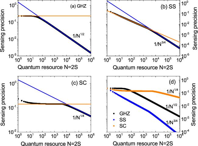
Figure 1. Frequency estimation precision $\delta \omega \sqrt{T}$ of a spin-S particle under collective dephasing by Ornstein–Uhlenbeck noise using three representative initial states: (a) cat state (GHZ), (b) maximal spin squeezed state (SS), (c) spin coherent state (SC). Black symbols for numerical results, solid lines for analytical results listed in the upper half of table 4 (the analytical results for SS and SC are valid only when N ≫ 1). Panel (d) compares the performance of the three initial states. The parameters are b = 1 (i.e., we take the noise magnitude b as the unit of the noise) and τc = 0.01. |
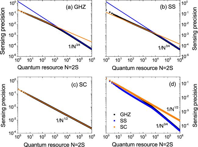
Figure 2. Frequency estimation precision $\delta \omega \sqrt{T}$ of a spin-S particle under individual dephasing by Ornstein–Uhlenbeck noise using three representative initial states: (a) cat state (GHZ), (b) maximal spin squeezed state (SS), (c) spin coherent state (SC). Black symbols for numerical results, solid lines for analytical results listed in the lower half of table 4 (the analytical results for SS are valid only when N ≫ 1). Panel (d) compares the performance of the three initial states. The parameters are b = 1 (i.e., we take the noise magnitude b as the unit of the noise) and τc = 0.01. |
As shown in figures 1(a)–(c) and 2(a)–(c), for N ≫ 1, the asymptotic analytical results agree with the numerical results for all initial states: GHZ, SS, and SC. Therefore, in the large-N limit, the N scaling is completely determined by the exponent β = 2 in the short-time expansion of the decoherence exponent χ(t) ≈ (b2/2)τ2, as discussed in the previous subsection.
Finally we give a general justification of the assumption χ(t) = αtβ for a general Gaussian noise $\tilde{\omega }(t)$ with no intrinsic frequency, so that C(t) ≈ C(0) for t ≪ τc and C(t) ≈ 0 for t ≫ τc. According to the definition equation (6 ), in the short-time regime t ≪ τc, equation (6 ) simplifies to 6 ) goes from 0 to t, only the integral from 0 to ∼ τc contributes, hence
$\begin{eqnarray*}\chi (t)\approx C(0){\int }_{0}^{t}{\rm{d}}\tau \,(t-\tau )=\frac{1}{2}C(0){t}^{2}\propto {t}^{2}.\end{eqnarray*}$
In the long-time regime t ≫ τc, although the integral in equation ( $\begin{eqnarray*}\chi (t)\approx t{\int }_{0}^{t}{\rm{d}}\tau \,C(\tau )\approx t{\int }_{0}^{+\infty }{\rm{d}}\tau \,C(\tau )\propto t.\end{eqnarray*}$
Collecting both cases gives the general behavior χ(t) ≈ αtβ with β = 2 for t ≪ τc and β = 1 for t ≫ τc. The Markovian limit τc → 0 corresponds to β = 1, while the extreme non-Markovian limit τc → ∞ corresponds to β = 2.4. Conclusion
Exploring the quantum advantages of various quantum sensors in noisy environments has been a central focus over recent years. In this context, high-spin particles (either naturally occurring or made from a collection of spin-1/2 particles) are prevalent quantum sensors for frequency estimation and three important states have been widely utilized: the spin coherent state (SC), the Schrödinger cat state or GHZ state, and the maximal spin squeezed state (SS). Existing works have mostly focused on their performance under individual dephasing, leaving collective dephasing unexplored. Here we provide a complete picture for the performance of GHZ, SS, and SC under both individual and collective dephasing by a general Gaussian noise. Surprisingly, we find that SC is worse than the classical scheme under collective dephasing, although it is equivalent to the classical scheme under individual dephasing. We further find that SS give the best precision in all cases. By contrast, the widely studied GHZ outperforms the classical scheme only under individual dephasing by non-Markovian noises. Our results establish the general advantage of SS for noisy frequency estimation based on two classes of quantum sensors (i.e., a collection of spin-1/2's or naturally occurring high-spin particles), and are relevant to many quantum sensing platforms.