


1. Introduction
In recent years, numerous modified gravitational theories have been presented to address various shortcomings of Einstein's General Relativity and to provide a more comprehensive understanding of the observed Universe. In particular, higher curvature gravity theories have emerged as effective tools for this purpose. These higher-order modifications to the Einstein-Hilbert action lead to the quantization of the field when studied in curved space-time [1]. Due to this attractive feature, many gravity theories involving higher-order derivative curvature terms have been developed in recent years. Among such theories, Lovelock gravity occupies a prominent place. Originally proposed by Lanczos [2], Lovelock [3, 4] further explored this subset of higher curvature gravity theories in the 1970s. One of the appealing features of Lovelock gravity is that its field equations contain derivatives of the metric components only up to the second order. Additional notable features include the preservation of Bianchi identities, which ensure the conservation of energy, i.e., ∇iTij = 0, and the ghost-free quantization of the linearized theory [5, 6].
These remarkable properties of Lovelock gravity establish it as the most natural generalization of Einstein's gravity in higher dimensions, making it an ideal framework for studying the effects of higher curvature terms on gravitational physics. In addition to the first two terms of the Lovelock Lagrangian, there is a third term, which is a combination of quadratic order curvature terms known as the Gauss–Bonnet (GB) term. This leads to the Einstein–Gauss–Bonnet (EGB) gravity, introducing modifications to the Einstein-Hilbert action, which correspond to the low-energy effective action of heterotic string theory [7, 8]. Furthermore, the GB term contributes to non-trivial dynamics in dimensions D > 4, allowing for the exploration of various physical phenomena [9]. For instance, Deser and Boulware [10] obtained a black hole solution in D≥5 dimensions of EGB theory. Additionally, several other types of physical phenomena have been explored within the context of higher curvature gravity [11–15]. Similarly, the gravitational collapse of a spherical dust cloud has been studied in [16–19], while in [20], quark stars in an anisotropic background have been investigated in the same framework.
On the other hand, the GB term in 4D is a topological invariant and, as a result, does not contribute to the gravitational dynamics. However, Glavan and Lin [21] proposed a novel approach to 4D EGB gravity, where they demonstrated the presence of non-trivial effects from the GB term in 4D. To achieve this, they rescaled the GB coupling constant as α → α/(D − 4) in a D-dimensional spacetime and then took the limit D → 4. Through this limiting process, Lovelock's theorem can be bypassed, and Ostrogradsky instability can be avoided [22]. Consequently, a new theory, termed 4D EGB gravity, was developed. Within this framework, a variety of physically motivated solutions have been established, including black hole solutions and their physical characteristics [23–28], as well as charged black holes [29, 30]. Black holes coupled with non-linear electrodynamics and magnetic charges have also been explored within this theory [31–33]. Furthermore, considering the significance of this novel gravity theory, observational data have been used to constrain the rescaled GB parameter [34–36].
The action of D-dimensional EGB theory is given by
$\begin{eqnarray*}{ \mathcal I }=\displaystyle \frac{{c}^{4}}{16\pi G}{\int }_{{ \mathcal M }}{{\rm{d}}}^{D}x\sqrt{-g}\left(R+\hat{\alpha }{{ \mathcal L }}_{{ \mathcal G }{ \mathcal B }}\right)+{{ \mathcal S }}_{\mathrm{matter}},\end{eqnarray*}$
In [20], the authors proposed incorporating the GB term into 4D gravity by rescaling the coupling constant. $\begin{eqnarray*}\hat{\alpha }=\frac{\alpha }{D-4}.\end{eqnarray*}$
It is evident that this quantity diverges in the limit D → 4; however, it is possible to extract non-trivial contributions from the higher-dimensional GB term in 4D [21]. This theory, known as 4D EGB gravity, has garnered significant attention in recent years (for a review see [39]). However, in the original proposal [21], the field equations contain ill-defined terms that result in the divergence of second-order perturbation equations around a Minkowski background [40, 41]. Moreover, this 4D limit leads to unphysical divergences in the on-shell action [42]. In [43, 44], it was also argued that the simple rescaling of the GB coupling, as initially proposed by Glavan and Lin, fails to produce covariant equations for a massless graviton in 4D. Several alternative approaches have been proposed to address the issues present in the original 4D EGB gravity. One of these improved theories involves a conformal regularization method that introduces a counter-term to remove the divergent aspects of the theory [45, 46]. Another approach relies on Kaluza-Klein reduction, where the higher-dimensional EGB theory is reduced with a scalar field φ, representing the size of a maximally symmetric internal space [47, 48]. In both methods, the resulting 4D actions obtained by rescaling $\hat{\alpha }\to \frac{\alpha }{D-4}$ fall within subclasses of Horndeski theories: the first leading to shift-symmetric Horndeski, and the second to non-shift-symmetric Horndeski theories. Interestingly, when the internal space is spatially flat, the effective 4D action derived from Kaluza-Klein reduction matches that from conformal regularization. Additionally, another regularization method has been suggested, in which the temporal diffeomorphism invariance is explicitly broken [49].It is observed that the stars of stellar mass around or above 8M⊙ undergo gravitational collapse and come out with the emergence of a white dwarf, neutron star (NS) or a black hole singularity. Among these stellar entities, NSs with neutron degeneracy pressure emerge as a more interesting end product of gravitational collapse. The internal structure and their physical properties, are a matter of high intrigue for researchers. Thus, they are always in search of realistic, viable and competent models to describe the inside matter of compact objects. It is commonly assumed that self-gravitating stellar objects are composed of isotropic matter, meaning that the radial pressure equals the tangential pressure. However, there has been significant interest among researchers in obtaining exact solutions for both static isotropic and anisotropic stellar distributions. Though isotropic models provide useful insights, however a comprehensive and realistic description of stellar structures often requires consideration of anisotropic solutions. Lemaitre [50] gave the concept of anisotropy, Bowers and Liang [51] extended this concept for locally anisotropic relativistic spheres such as the pressure anisotropy on NSs. Ruderman [52] in 1972 put forward his observation that nuclear matter acts as anisotropic matter at a higher density of order 1015 g cm-3. According to the conjecture given by Herrera and Santos [53], anisotropic compact stars live in a powerful gravitational field.
The evaluation of compact stars is an important area of current research in General Relativity. Researchers have encountered numerous challenges in studying anisotropic matter in spherically symmetric objects, such as boson stars [54], gravastars [55], and NSs [56], along with various other stellar types. Scientists have proposed finding exact solutions for anisotropic stellar models across different gravitational frameworks. The behavior of two-fluid dark matter as anisotropic matter has been investigated for compact stars [57]. Additionally, slowly rotating anisotropic stars have been considered in [58], and anisotropic polystars have been introduced in [59–61]. Moreover, the demonstration of anisotropic superdense matter has shown that it can significantly alter the physical properties of relativistic stellar objects [62, 63]. Pressure anisotropy impacts the properties of NSs, including stability and the mass-radius relation [64]. Deriving anisotropic solutions is challenging due to the presence of non-linear terms in EFEs. Various methods have been employed to obtain exact anisotropic solutions for self-gravitating systems. In this context, gravitational decoupling (GD) presents an interesting technique for achieving anisotropic solutions. GD has two versions: the extended geometric deformation (EGD) approach and the minimal geometric deformation (MGD) approach. In the EGD approach, both the radial and temporal metric potentials are deformed, while in the MGD approach, only the radial metric potential is deformed, leaving the temporal metric potential unchanged.
The MGD approach is significant for calculating feasible solutions of spherically symmetric relativistic stellar configurations. This approach was proposed by Ovalle [65] to decouple gravitational sources and to study the exterior of spherically symmetric spacetime with perfect fluid under RS brane-world gravity [66]. Various astrophysical objects have been examined using this innovative approach [67–69]. MGD decoupling can yield deformed solutions of the Einstein equations [70, 71], which is challenging due to the presence of non-linear terms in the matter fields [72–88]. The inverse problem was discussed in [89], while completely deformed spacetimes were explored in [90]. Furthermore, black hole solutions related to this approach were analyzed in [91–94], and non-rotating black holes can be transformed into rotating ones, as discussed in [95, 96].
This article is organized as follows: section 2 provides a brief review of the major aspects related to GD and EGB gravitational field equations. In section 3 , we discuss the MGD approach, which transforms the field equations into two parts by modifying the radial metric component. This section includes two subsections that present the solutions of the standard EGB gravitational field equations and the field equations related to the additional sector through the mimicking of pressure. Section 4 explores the junction conditions. Section 5 offers a comprehensive physical analysis, examining matter variables, and equation of state parameters. The energy conditions, the square of the speed of sound, TOV equation and the adiabatic index are discussed in sections 6 , 7 , 8 , 9 , respectively. Finally, section 10 concludes our findings.
2. EGB gravitational field equations
We start this section by taking into account the modified action of D-dimensional EGB gravity, i.e., 1 ), ${{ \mathcal S }}_{\mathrm{matter}}$ is the Lagrangian of anisotropic matter, which depends on metric tensor gij only and is independent of its derivatives. By varying (1 ) with respect to metric tensor gij, the gravitational field equations are derived as 3 ) the Einstein tensor Gij and the contribution to the GB term Hij are defined as
$\begin{eqnarray}{ \mathcal I }=\displaystyle \frac{{c}^{4}}{16\pi G}{\int }_{{ \mathcal M }}{{\rm{d}}}^{D}x\sqrt{-g}\left(R+\displaystyle \frac{\alpha }{D-4}{{ \mathcal L }}_{{ \mathcal G }{ \mathcal B }}\right)+{{ \mathcal S }}_{\mathrm{matter}},\end{eqnarray}$
where R and g are 4-dimensional Ricci scalar and determinant of metric tensor gij, respectively. Moreover, α is the GB coupling constant of [Length]2, and ${{ \mathcal L }}_{{ \mathcal G }{ \mathcal B }}$ is the GB Lagrangian in the action, which is a specific combination of Ricci Scalar, Ricci tensor, and Riemann tensors, given by $\begin{eqnarray}{{ \mathcal L }}_{{ \mathcal G }{ \mathcal B }}={R}^{ijpq}{R}_{ijpq}-4{R}^{ij}{R}_{ij}+{R}^{2}.\end{eqnarray}$
In action ( $\begin{eqnarray}{G}_{ij}+\displaystyle \frac{\alpha }{D-4}{H}_{ij}=8\pi {T}_{ij}^{(\mathrm{tot})},\end{eqnarray}$
where ${T}_{ij}^{(\mathrm{tot})}$ is the total energy-momentum tensor (EMT) defined as $\begin{eqnarray}{T}_{ij}^{(\mathrm{tot})}={T}_{ij}+\beta {\theta }_{ij},\end{eqnarray}$
with $\begin{eqnarray}\begin{array}{l}{T}_{ij}=-\displaystyle \frac{2}{\sqrt{-g}}\displaystyle \frac{\partial (\sqrt{-g}{{ \mathcal L }}_{{\rm{m}}})}{\partial {g}^{ij}},\quad \mathrm{and}\\ {\theta }_{ij}=\displaystyle \frac{2}{\sqrt{-g}}\displaystyle \frac{\partial (\sqrt{-g}{{ \mathcal L }}_{\theta })}{\partial {g}^{ij}}.\end{array}\end{eqnarray}$
Here ${{ \mathcal L }}_{{\rm{m}}}$ and ${{ \mathcal L }}_{\theta }$ are the Lagrangian of matter field and extra source, respectively. Furthermore, in equation ( $\begin{eqnarray}{G}_{ij}={R}_{ij}-\frac{1}{2}{g}_{ij}R,\end{eqnarray}$
$\begin{eqnarray}\begin{array}{rcl}{H}_{ij} & = & 2\left(R{R}_{ij}-2{R}_{ip}{R}_{j}^{p}-2{R}_{ijpq}{R}^{pq}-{R}_{ipqk}{R}_{j}^{pqk}\right)\\ & & -\,\frac{1}{2}{g}_{ij}{{ \mathcal L }}_{{ \mathcal G }{ \mathcal B }}.\end{array}\end{eqnarray}$
Now, we consider the spacetime, which represents interior geometry of static and spherically symmetric source $\begin{eqnarray}{\rm{d}}{s}_{4}^{2}=-{{\rm{e}}}^{2\phi (r)}{\rm{d}}{t}^{2}+{{\rm{e}}}^{2\lambda (r)}{\rm{d}}{r}^{2}+{r}^{2}{\rm{d}}{\theta }^{2}+{r}^{2}{\sin }^{2}\theta {\rm{d}}{\varphi }^{2},\end{eqnarray}$
where φ(r) and λ(r) are the metric potentials which depend on radial coordinate r. Moreover, the mathematical form of EMT for anisotropic fluid distribution is defined as $\begin{eqnarray}{T}_{ij}=(\rho +{p}_{{\rm{r}}}){u}_{i}{u}_{j}+{p}_{t}{g}_{ij}+({p}_{{\rm{r}}}-{p}_{{\rm{t}}}){\chi }_{i}{\chi }_{j},\end{eqnarray}$
where ρ is the matter energy density, pr and pt are the radial and tangential pressures, ui is the four-vector and χj is spacelike unit vector in the direction of radial component r which satisfy χjχj = − uiui = 1. Now we see the total EMT ${T}_{ij}^{(\mathrm{tot})}$ takes the form as follows $\begin{eqnarray}{T}_{ij}^{(\mathrm{tot})}=(\varepsilon +{P}_{\perp }){u}_{i}{u}_{j}+{P}_{\perp }{g}_{ij}+({P}_{{\rm{r}}}-{P}_{\perp }){\chi }_{i}{\chi }_{j},\end{eqnarray}$
where we have $\varepsilon =\rho +\beta {\theta }_{0}^{0}$ as the energy density of total EMT, ${P}_{{\rm{r}}}={p}_{{\rm{r}}}-\beta {\theta }_{1}^{1}$ and ${P}_{\perp }={p}_{{\rm{t}}}-\beta {\theta }_{2}^{2}$ are the total radial and tangential pressures, respectively. The additional source θij modifies the anisotropy in Tij. However, the physical nature of θij is not explicitly defined. The formalism is designed to be general, which allows for a wide range of possible interpretations of θij. It could represent contributions from various types of matter or fields, for example, exotic matter, higher-dimensional gravitational effects, or even quantum fields. The formalism does not provide a clear answer to what type of external field could induce the minimal geometric deformation of solutions. However, it is mathematically possible to decouple and analyze the effects of θij, the specific field whether it be scalar, vector, tensor, or other exotic fields that correspond to this energy-momentum tensor is not identified within the formalism itself. This means that the MGD method is more of a framework for handling additional fields, rather than providing a clear physical interpretation of those fields.Since both Einstein tensor Gij and GB tensor Hij are divergence free, the total EMT in (3 ) is also guaranteed to be divergence free. Thus, we have 8 ), under 4D EGB gravity. Now, using equations (8 ) and (10 ) with equations (3 ) and (4 ), we have the non-zero components of gravitational field equations as follows 11 ) takes the form as
$\begin{eqnarray}{{\rm{\nabla }}}^{i}{T}_{{ij}}^{({\rm{tot}})}=0.\end{eqnarray}$
The divergence of EMT yields the following conservation equation $\begin{eqnarray}{\phi }^{{\prime} }(\varepsilon +{P}_{{\rm{r}}})+{P}_{{\rm{r}}}^{{\prime} }+\frac{2}{{\rm{r}}}({P}_{{\rm{r}}}-{P}_{\perp })=0.\end{eqnarray}$
The above-stated equation is also termed as the general hydrostatic equation for spacetime ( $\begin{eqnarray}\begin{array}{rcl}8\pi \varepsilon & = & 8\pi (\rho +\beta {\theta }_{0}^{0})=\frac{2\lambda ^{\prime} {{\rm{e}}}^{-2\lambda }}{r}\left(1+\frac{2\alpha (1-{{\rm{e}}}^{-2\lambda })}{{r}^{2}}\right)\\ & & +\,\frac{1-{{\rm{e}}}^{-2\lambda }}{{r}^{2}}\left(1-\frac{\alpha (1-{{\rm{e}}}^{-2\lambda })}{{r}^{2}}\right),\end{array}\end{eqnarray}$
$\begin{eqnarray}\begin{array}{rcl}8\pi {P}_{r} & = & 8\pi ({p}_{r}-\beta {\theta }_{1}^{1})=\frac{2\phi ^{\prime} {{\rm{e}}}^{-2\lambda }}{r}\left(1+\frac{2\alpha (1-{{\rm{e}}}^{-2\lambda })}{{r}^{2}}\right)\\ & & -\,\frac{1-{{\rm{e}}}^{-2\lambda }}{{r}^{2}}\left(1-\frac{\alpha (1-{{\rm{e}}}^{-2\lambda })}{{r}^{2}}\right),\end{array}\end{eqnarray}$
$\begin{eqnarray}\begin{array}{rcl}8\pi {P}_{\perp } & = & 8\pi ({p}_{t}-\beta {\theta }_{2}^{2})\\ & = & \frac{{{\rm{e}}}^{-4\lambda }}{{r}^{4}}[2\alpha {{\rm{e}}}^{2\lambda }+r({{\rm{e}}}^{2\lambda }({r}^{2}-2\alpha +2\alpha )\phi ^{\prime} )\\ & & +{r}^{2}(-2\alpha +{{\rm{e}}}^{2\lambda }({r}^{2}+2\alpha )){\phi }^{{\prime} 2}\\ & & -r\lambda ^{\prime} ({{\rm{e}}}^{2\lambda }({r}^{2}-2\alpha )+2\alpha \\ & & +r(-6\alpha +{{\rm{e}}}^{2\lambda }({r}^{2}+2\alpha ))\phi ^{\prime} )-\alpha -{{\rm{e}}}^{4\lambda }\\ & & +{r}^{2}({{\rm{e}}}^{2\lambda }{r}^{2}-2\alpha +2{{\rm{e}}}^{2\lambda }\alpha )\phi ^{\prime\prime} ],\end{array}\end{eqnarray}$
where prime represents the derivative of metric potentials with respect to radial coordinate r. For the decoupled anisotropic fluid source, the conservation equation ( $\begin{eqnarray}\begin{array}{rcl} & & {\phi }^{{\prime} }(\rho +{p}_{{\rm{r}}})+{p}_{{\rm{r}}}^{{\rm{{\prime} }}}+\displaystyle \frac{2}{r}({p}_{{\rm{r}}}-{p}_{{\rm{t}}})\\ & & \quad +\,\beta \left[\phi ^{\prime} ({\theta }_{0}^{0}-{\theta }_{1}^{1})-({\theta }_{1}^{1})^{\prime} -\displaystyle \frac{3}{r}({\theta }_{1}^{1}-{\theta }_{2}^{2})\right]=0.\end{array}\end{eqnarray}$
Since the extra gravitational source θij demonstrates the anisotropy in the internal matter of a self-gravitating system, the anisotropic factor is expressed as follows $\begin{eqnarray}{\bigtriangleup }^{(\mathrm{tot})}=8\pi ({P}_{\perp }-{P}_{{\rm{r}}}).\end{eqnarray}$
Moreover, the evaluation of gravitational mass function m(r) is performed using the expression stated below in 4D EGB gravity. $\begin{eqnarray}m(r)=4\pi {\int }_{0}^{r}\rho (r){r}^{2}{\rm{d}}r.\end{eqnarray}$
3. GD via the MGD approach
The metric functions are geometrically deformed to incorporate the source θij in the following manner 20 ) via the source θij. By applying the linear transformation (20 ) on the EGB gravitational field equations (13 )-(15 ), two sets of equations are obtained. Consider the case when β = 0, which gives us the standard EGB gravitational system of equations that depends on the gravitational metric potentials μ and φ as follows
$\begin{eqnarray}\phi (r)\to \eta (r)+\beta h(r),\end{eqnarray}$
$\begin{eqnarray}{{\rm{e}}}^{-2\lambda (r)}\to \mu (r)+\beta f(r).\end{eqnarray}$
Here h(r) and f(r) are the geometric deformation functions that introduce deformations in the radial and temporal metric potentials, respectively, while β is the dimensionless deformation control parameter. The metric components are minimally deformed, allowing for two possibilities: either we set h(r) ≠ 0 paired with f(r) = 0 or the h(r) = 0 paired with f(r) ≠ 0. We consider the latter case, where only the radial metric potential is deformed while the temporal component remains unchanged. This indicates that anisotropy is introduced into the system through radial deformation ( $\begin{eqnarray}8\pi \rho =-\frac{(-1+\mu )({r}^{2}-\alpha +\alpha \mu )+r({r}^{2}+2\alpha -2\alpha \mu )\mu ^{\prime} }{{r}^{4}},\end{eqnarray}$
$\begin{eqnarray}8\pi {p}_{r}=\frac{-{r}^{2}+\alpha +{\mu }^{2}(\alpha -4r\alpha \phi ^{\prime} )+\mu ({r}^{2}-2\alpha +2({r}^{3}+2r\alpha )\phi ^{\prime} )}{{r}^{4}},\end{eqnarray}$
$\begin{eqnarray}\begin{array}{rcl}8\pi {p}_{t} & = & \frac{1}{2{r}^{4}}[-2\alpha +r\mu ^{\prime} ({r}^{2}\\ & & -2\alpha +({r}^{3}+2r\alpha )\phi ^{\prime} )-2\alpha {\mu }^{2}(1-2r\phi ^{\prime} \\ & & +2{r}^{2}{\phi }^{{\prime} 2}+2{r}^{2}\phi ^{\prime\prime} )\\ & & +2\mu (2\alpha +)({r}^{3}-2r\alpha )\phi ^{\prime} +({r}^{4}+2{r}^{2}\alpha ){\phi }^{{\prime} 2}\\ & & +r\alpha \mu ^{\prime} (1-3r\phi ^{\prime} )+{r}^{4}\phi ^{\prime\prime} +2{r}^{2}\alpha \phi ^{\prime\prime} )].\end{array}\end{eqnarray}$
Hence, the interior spacetime becomes $\begin{eqnarray}{\rm{d}}{s}^{2}=-{{\rm{e}}}^{2\phi (r)}{\rm{d}}{t}^{2}+\frac{{\rm{d}}{r}^{2}}{\mu (r)}+{r}^{2}{\rm{d}}{\theta }^{2}+{r}^{2}{\sin }^{2}\theta {\rm{d}}{\varphi }^{2}.\end{eqnarray}$
Here, we have second set of field equation with β ≠ 0 containing the source θij and the unknowns μ, φ, f, i.e., $\begin{eqnarray}\begin{array}{rcl}8\pi {\theta }_{0}^{0} & = & \frac{1}{{r}^{4}}[-\alpha \beta {f}^{2}-r({r}^{2}+2\alpha -2\alpha \mu )f^{\prime} \\ & & +\,f(-{r}^{2}+2\alpha -2\alpha \mu +2r\alpha \beta f^{\prime} +2r\alpha \mu ^{\prime} )],\end{array}\end{eqnarray}$
$\begin{eqnarray}\begin{array}{rcl}8\pi {\theta }_{1}^{1} & = & -\frac{f}{{r}^{4}}[{r}^{2}-2\alpha +2{r}^{3}\phi ^{\prime} +4r\alpha \phi ^{\prime} \\ & & +\,\alpha \beta f(1-4r\phi ^{\prime} )+\mu (2\alpha -8r\alpha \phi ^{\prime} )],\end{array}\end{eqnarray}$
$\begin{eqnarray}\begin{array}{rcl}8\pi {\theta }_{2}^{2} & = & -\frac{1}{2{r}^{4}}[rf^{\prime} ({r}^{2}-2\alpha +({r}^{3}+2r\alpha )\phi ^{\prime} \\ & & +\,\mu (2\alpha -6r\alpha \phi ^{\prime} ))\\ & & -\,2\alpha \beta {f}^{2}(1-2r\phi ^{\prime} +2{r}^{2}{\phi }^{{\prime} 2}+2{r}^{2}\phi ^{\prime\prime} )\\ & & +\,2f(2\alpha +r\alpha \mu ^{\prime} +{r}^{3}\phi ^{\prime} -2r\alpha \phi ^{\prime} \\ & & -3{r}^{2}\alpha \mu ^{\prime} \phi ^{\prime} \\ & & +\,{r}^{4}{\phi }^{{\prime} 2}\\ & & +\,2{r}^{2}\alpha {\phi }^{{\prime} 2}+r\alpha \beta f^{\prime} (1-3r\phi ^{\prime} )+{r}^{4}\phi ^{\prime\prime} \\ & & +\,2{r}^{2}\alpha \phi ^{\prime\prime} -2\alpha \mu (1-2r\phi ^{\prime} +2{r}^{2}{\phi }^{{\prime} 2}+2{r}^{2}\phi ^{\prime\prime} ))].\end{array}\end{eqnarray}$
3.1. Minimally deformed solution in 4D EGB gravity
Now, we consider an exact solution named the 'Tolman–Finch–Skea (TFS)' solution, given by 21 )-(23 ) take the following particular forms 25 )-(27 ), which is based on the evaluation of decoupling function f(r).
$\begin{eqnarray}\phi (r)=2\cdot \mathrm{ln}[B(1+A{r}^{2})]\quad \mathrm{and}\quad \mu (r)=\displaystyle \frac{1}{1+C{r}^{2}},\end{eqnarray}$
where C and A are constants of [Length]2 and B is a dimensionless constant. The choice of the TFS model in 4D EGB gravity is motivated by its regularity, stability, and capacity to model realistic stellar structures, including anisotropy. Its adaptability, smooth matching to exterior solutions, and use as a reference for evaluating new predictions makes it an ideal candidate for studying the effects of modifications in strong gravitational fields, especially in the context of compact stars. With this consideration, equations ( $\begin{eqnarray}8\pi \rho =\frac{C(3+C(4{r}^{2}+3\alpha )+{C}^{2}(-{r}^{4}+{r}^{2}\alpha ))}{{(1+C{r}^{2})}^{3}},\end{eqnarray}$
$\begin{eqnarray}8\pi {p}_{r}=\frac{[C(-1+C({r}^{2}+\alpha ))+A(8+C(7{r}^{2}+16\alpha )+{C}^{2}(-{r}^{4}+{r}^{2}\alpha ))]}{(1+A{r}^{2}){(1+C{r}^{2})}^{2}},\end{eqnarray}$
$\begin{eqnarray}\begin{array}{rcl}8\pi {p}_{t} & = & \frac{1}{(1+A{r}^{2}){(1+C{r}^{2})}^{3}}[-C(1+C({r}^{2}-\alpha )+{C}^{2}{r}^{2}\alpha )\\ & & +\,2A(4-{C}^{3}{r}^{4}\alpha +C(5{r}^{2}+8\alpha ))\\ & & +\,{A}^{2}{r}^{2}(16-{C}^{3}{r}^{4}\alpha +C(27{r}^{2}+32\alpha )\\ & & +\,{C}^{2}(11{r}^{4}+9{r}^{2}\alpha ))].\end{array}\end{eqnarray}$
Next, we will adopt mimicking constraint for pressure to solve the second system of equations (3.2. Mimicking of pressure constraint i.e. ${p}_{r}={\theta }_{1}^{1}$ and deformation function
Here, we consider the radial component of the θ-sector to be equal to the seed radial pressure because, in this scenario, the deformation introduced is sufficiently small, ensuring that the original or seed configuration remains largely unaffected. The goal of minimal geometric deformation is to keep the main features of the seed metric, such as pressure and other physical properties, preserved. This means the deformation is not strong enough to significantly affect the radial component, so the radial pressure in the deformed state remains close to the seed radial pressure. Using this constraint in equation (22 ) and further solving with equation (26 ), we have the quadratic equation in f(r), given below 28 ), the above expression for f(r) leads to the following form 28 ) and f (34 ) into equations (25 )–(27 ).
$\begin{eqnarray}\begin{array}{rcl}0 & = & [\alpha \beta (1-4r\phi ^{\prime} )]{f}^{2}+[{r}^{2}-2\alpha +2{r}^{3}\phi ^{\prime} \\ & & +\,4r\alpha \phi ^{\prime} +\mu (2\alpha -8r\alpha \phi ^{\prime} )]f\\ & & +\,[\alpha -r+{\mu }^{2}(\alpha -4r\alpha \phi ^{\prime} )\\ & & +\,\mu ({r}^{2}-2\alpha +2({r}^{3}+2r\alpha )\phi ^{\prime} )].\end{array}\end{eqnarray}$
Solving the above quadratic equation we have the following expression for decoupling function f(r) in terms of φ and ν as follows $\begin{eqnarray}\begin{array}{rcl}f & = & \frac{1}{2\alpha \beta (-1+4r\phi ^{\prime} )}[{r}^{2}-2\alpha +2\alpha \mu +2{r}^{3}\phi ^{\prime} +4r\alpha \phi ^{\prime} \\ & & -\,8r\alpha \mu \phi ^{\prime} +(({r}^{2}-2\alpha +2({r}^{3}+2r\alpha )\phi ^{\prime} \\ & & +\,\mu (2\alpha -8r\alpha \phi ^{\prime} ){)}^{2}+4\alpha \beta (1-4r\phi ^{\prime} )\\ & & \times \,({r}^{2}-\alpha +\alpha {\mu }^{2}(-1+4r\phi ^{\prime} )\\ & & -\,\mu ({r}^{2}-2\alpha +2({r}^{3}+2r\alpha )\phi ^{\prime} )){)}^{\frac{1}{2}}].\end{array}\end{eqnarray}$
Now by taking into account the expressions given in equation ( $\begin{eqnarray}\begin{array}{rcl}f & = & \frac{({r}^{4}+A{r}^{6})}{2\alpha \beta (1-15A{r}^{2})}\left[-\frac{1}{{r}^{2}}-\frac{8A}{1+A{r}^{2}}+\frac{2\alpha }{{r}^{4}}-\frac{16\alpha A}{{r}^{2}+A{r}^{4}}\right.\\ & & \left.-\,\frac{2\alpha }{{r}^{4}+C{r}^{6}}+\frac{32\alpha A}{{r}^{2}+A{r}^{4}+C{r}^{4}+AC{r}^{6}}-\sqrt{\omega }\right],\end{array}\end{eqnarray}$
where $\begin{eqnarray*}\begin{array}{rcl}\omega & = & \frac{1}{{r}^{4}{(1+A{r}^{2})}^{2}{(1+C{r}^{2})}^{2}}(1+2C({r}^{2}+2\alpha (-1+\beta ))\\ & & +\,{C}^{2}({r}^{4}+4{r}^{2}\alpha (-1+\beta )-4{\alpha }^{2}(-1+\beta ))\\ & & +\,{A}^{2}(81{C}^{2}{r}^{8}+256{\alpha }^{2}+6C{r}^{6}(27+2C\alpha (21-5\beta ))\\ & & +\,32{r}^{2}\alpha (-9+15\beta +2C\alpha (-7+15\beta ))\\ & & +\,{r}^{4}(81+4{C}^{2}{\alpha }^{2}(49+a5\beta )+12C\alpha (-3+35\beta )))\\ & & +\,2A(9{C}^{2}{r}^{6}-16\alpha (1+2C\alpha (-1+\beta )+\beta )\\ & & +\,{r}^{2}(9+28{C}^{2}\alpha (-1+\beta )-4C\alpha (5+11\beta ))\\ & & -\,2C{r}^{4}(-9+2C(\alpha +7\alpha \beta )))).\end{array}\end{eqnarray*}$
Now, one can easily get the expressions for θij components by inserting the values of φ, μ (4. Exterior spacetime and junction conditions for TFS solution
Now, the boundary conditions need to be set for the obtained solutions. Thus, we equate the interior manifold ${{ \mathcal M }}^{-}$ given in equation (28 ) to the exterior solution proposed by Glavan and Lin for the limit n → 4, given by 8 ) and (35 ) should be matched smoothly across the boundary. The corresponding timelike hyper-surface is given by
$\begin{eqnarray}{\rm{d}}{s}^{2}=-F(r){\rm{d}}{t}^{2}+{[F(r)]}^{-1}{\rm{d}}{r}^{2}+{r}^{2}{\rm{d}}{\theta }^{2}+{r}^{2}{\sin }^{2}\theta {\rm{d}}{\varphi }^{2},\end{eqnarray}$
where $\begin{eqnarray}F(r)=1+\frac{{r}^{2}}{32\alpha \pi }\left(1-\sqrt{1+\frac{128\alpha \pi M}{{r}^{3}}}\right).\end{eqnarray}$
Here, M denotes the total gravitational mass. The line elements ( $\begin{eqnarray}{\rm{d}}{s}_{{\rm{\Sigma }}}^{2}=-{\rm{d}}{\tau }^{2}+{R}^{2}({\rm{d}}{\theta }^{2}+{\sin }^{2}\theta {\rm{d}}{\varphi }^{2}),\end{eqnarray}$
with the intrinsic co-ordinates χm = (τ, θ, φ) in Σ and τ is the proper time at the boundary. Taking into account the field equations projected on the surface Σ which are basically generalized forms of Darmois-Israel conditions for EGB gravity theory (see[97, 98]) $\begin{eqnarray}\begin{array}{rcl} & & 2\langle {K}_{mn}-K{h}_{mn}\rangle +4\alpha \langle 3{J}_{mn}-J{h}_{mn}\\ & & \quad +\,2{P}_{mpqn}{K}^{pq}\rangle =-{\kappa }^{2}{S}_{mn},\end{array}\end{eqnarray}$
where ⟨·⟩ is the jump across the hyper-surface Σ of the given quantity. The induced metric on Σ is hmn = gmn − nmnn, while the free of divergence part Pmnpq of the Riemann tensor can be stated as $\begin{eqnarray}\begin{array}{rcl}{P}_{mnpq} & = & {R}_{mnpq}+({R}_{np}{h}_{qm}-{R}_{nq}{h}_{pn})\\ & & -\,({R}_{mp}{h}_{qn}-{R}_{mq}{h}_{pn})+\frac{1}{2}R({h}_{mp}{h}_{qn}-{h}_{mq}{h}_{pn}),\end{array}\end{eqnarray}$
and here J is the trace of $\begin{eqnarray}\begin{array}{rcl}{J}_{mn} & = & \frac{1}{3}[2K{K}_{mp}{K}_{n}^{p}+{K}_{pq}{K}^{pq}{K}_{mn}\\ & & -\,2Kmp{K}^{pq}{K}_{qn}-{K}^{2}{K}_{mn}].\end{array}\end{eqnarray}$
The extrinsic curvature takes the form as $\begin{eqnarray}{K}_{mn}^{\pm }=-{n}_{\gamma }^{\pm }{\left(\frac{{\partial }^{2}{X}^{\gamma }}{\partial {\chi }^{m}\partial {\chi }^{n}}+{{\rm{\Gamma }}}_{\mu \nu }^{\gamma }\frac{\partial {X}^{\mu }}{\partial {\chi }^{m}}\frac{\partial {X}^{\nu }}{\partial {\chi }^{n}}\right)}_{r=R},\end{eqnarray}$
with χm being the intrinsic co-ordinates of the hyper-surface and the signature ± depends on the signature of the junction hyper-surface.Furthermore, the interior geometry under GD through the minimal deformation technique is 28 ). Now, we are going to analyze the junction of inner and outer surfaces. The continuity of the Ist fundamental form at the outer boundary gives ${g}_{tt}^{-}={g}_{tt}^{+}$ and ${g}_{rr}^{-}={g}_{rr}^{+}$, with '-' and '+' indicates the inner and outer spacetime, which are further elaborated as 24 ). Now taking into account this expression of μ(R) together with equation (44 ), we get the mass function as 3 ) can take the form as 26 ) into (50 ), and obtain the following expression 26 ) in equation (51 ), we find 8 ) to static spherically symmetric exterior vacuum solution shown in (53 ). For the exterior geometry, we must have f⋆(R) = 0 in (53 ). Consequently, we have 43 ) and (49 ), and find the following expressions
$\begin{eqnarray}{\rm{d}}{s}^{2}=-{{\rm{e}}}^{2\phi (r)}{\rm{d}}{t}^{2}+\frac{{\rm{d}}{r}^{2}}{f(r)+\mu (r)}+{r}^{2}{\rm{d}}{\theta }^{2}+{r}^{2}{\sin }^{2}\theta {\rm{d}}{\varphi }^{2},\end{eqnarray}$
where φ and μ are given by equation ( $\begin{eqnarray}{{\rm{e}}}^{2{\phi }^{-}}{| }_{r=R}={{\rm{e}}}^{2{\phi }^{+}}{| }_{r=R}\quad {\rm{a}}{\rm{n}}{\rm{d}}\quad {{\rm{e}}}^{2{\lambda }^{-}}{| }_{r=R}={{\rm{e}}}^{2{\lambda }^{+}}{| }_{r=R},\end{eqnarray}$
which yields $\begin{eqnarray}\begin{array}{rcl}{{\rm{e}}}^{-2\lambda (R)} & = & \beta f(R)+\mu (R)\\ & = & \left[1+\frac{{R}^{2}}{32\alpha \pi }\left(1-\sqrt{1+\frac{128\alpha \pi M}{{R}^{3}}}\right)\right],\\ {{\rm{e}}}^{2\phi (R)} & = & \left[1+\frac{{R}^{2}}{32\alpha \pi }\left(1-\sqrt{1+\frac{128\alpha \pi M}{{R}^{3}}}\right)\right].\end{array}\end{eqnarray}$
Here, $\mu (R)=1+\frac{{R}^{2}}{32\alpha \pi }\left(\right.1-\sqrt{1+\frac{128\alpha \pi {M}_{{\rm{E}}{\rm{G}}{\rm{B}}}}{{R}^{3}}}\left)\right.$, where MEGB = mEGB(R) denotes total mass of stellar object in the non-deformed spacetime ( $\begin{eqnarray}\begin{array}{rcl}M & = & {M}_{{\rm{E}}{\rm{G}}{\rm{B}}}+\frac{1}{2R}\beta f(R)\left[\right.16\pi \alpha \beta f(R)\\ & & -\,\sqrt{R({R}^{3}+128\alpha \pi {M}_{{\rm{E}}{\rm{G}}{\rm{B}}})}\left]\right..\end{array}\end{eqnarray}$
On the other side the extrinsic curvature or the continuity of second fundamental form leads to the following condition $\begin{eqnarray}{[({G}_{ij}+\alpha {H}_{ij}){r}^{j}]}_{r=R}=0,\end{eqnarray}$
where rj is radial unit vector. So equation ( $\begin{eqnarray}{[{T}_{ij}{r}^{j}]}_{r=R}=0,\end{eqnarray}$
which implies $\begin{eqnarray}{[{P}_{{\rm{r}}}]}_{r=R}=0.\end{eqnarray}$
It can be written as $\begin{eqnarray}{[{p}_{{\rm{r}}}-\beta {\theta }_{1}^{1}]}_{r=R}=0.\end{eqnarray}$
Here, the above junction condition takes the final form which is the generalized second fundamental condition: $\begin{eqnarray}{p}_{{\rm{r}}}(R)-\beta {({\theta }_{1}^{1})}^{-}(R)=-\beta {({\theta }_{1}^{1})}^{+}(R),\end{eqnarray}$
where ${({\theta }_{1}^{1})}^{+}(R)$ and ${({\theta }_{1}^{1})}^{-}(R)$ are the θ-components of exterior and interior spacetimes, respectively. Now we plug the expression of ${\theta }_{1}^{1}$ from ( $\begin{eqnarray}{p}_{r}(R)+\frac{\beta {f}_{R}({R}^{4}-2\alpha +\alpha \beta {f}_{R}+2\alpha {\mu }_{R}+{\phi }_{R}^{{\prime} }R(2{R}^{2}+4\alpha -4\alpha \beta {f}_{R}-8\alpha {\mu }_{R}))}{8\pi {R}^{4}}=-\beta {({\theta }_{1}^{1})}^{+}(R),\end{eqnarray}$
where we have used the notations as ${\phi }_{R}^{{\prime} }={\partial }_{r}\phi {| }_{r=R}$, μR = μ(R) and fR = f(R). For the outer geometry, using equation ( $\begin{eqnarray}\begin{array}{rcl} & & {p}_{r}(R)+\frac{\beta {f}_{R}({R}^{4}-2\alpha +\alpha \beta {f}_{R}+2\alpha {\mu }_{R}+{\phi }_{R}^{{\prime} }R(2{R}^{2}+4\alpha -4\alpha \beta {f}_{R}-8\alpha {\mu }_{R}))}{8\pi {R}^{4}}\\ & & \quad =\frac{\beta {f}_{R}^{\star }}{8\pi {R}^{4}}\left[{R}^{4}-2\alpha +\alpha \beta {f}_{R}^{\star }+2\alpha \left[1+\frac{{R}^{2}}{32\alpha \pi }\right.\right.\\ & & \times \left.\left(1-\sqrt{1+\frac{128\alpha \pi M}{{R}^{3}}}\right)\right]\\ & & \quad +\,R\left(\frac{32\alpha \pi M+{R}^{3}\left(1-\sqrt{1+\frac{128\alpha \pi M}{{R}^{3}}}\right)}{{R}^{2}\sqrt{1+\frac{128\alpha \pi M}{{R}^{3}}}\left[-32\alpha \pi +{R}^{2}\left(-1+\sqrt{1+\frac{128\alpha \pi M}{{R}^{3}}}\right)\right]}\right)\\ & & \quad \times \left(2{R}^{2}+4\alpha -4\alpha \beta {f}_{R}^{\star }-8\alpha \right.\\ & & \quad \left.\left.\left[1+\frac{{R}^{2}}{32\alpha \pi }\left(1-\sqrt{1+\frac{128\alpha \pi M}{{R}^{3}}}\right)\right]\right)\right],\end{array}\end{eqnarray}$
where ${f}_{R}^{\star }={f}^{\star }(R)$ represents the deformation function for the outer spacetime at r = R. The 4D spacetime can be defined as $\begin{eqnarray}\begin{array}{rcl}{\rm{d}}{s}^{2} & = & -\left[1+\frac{{r}^{2}}{32\alpha \pi }\left(1-\sqrt{1+\frac{128\alpha \pi M}{{r}^{3}}}\right)\right]{\rm{d}}{t}^{2}\\ & & +\,{\left[1+\frac{{r}^{2}}{32\alpha \pi }\left(1-\sqrt{1+\frac{128\alpha \pi M}{{r}^{3}}}\right)+\beta {f}^{\star }(r)\right]}^{-}{\rm{d}}{r}^{2}\\ & & +\,{r}^{2}{\rm{d}}{\theta }^{2}+{\sin }^{2}{\theta }^{2}{\rm{d}}{\varphi }^{2}.\end{array}\end{eqnarray}$
All the above mentioned conditions are sufficient and necessary for matching the MGD metric ( $\begin{eqnarray}{P}_{r}(R)={p}_{{\rm{r}}}(R)+\displaystyle \frac{\beta {f}_{R}({R}^{4}-2\alpha +\alpha \beta {f}_{R}+2\alpha {\mu }_{R}+{\phi }_{R}^{^{\prime} }R(2{R}^{2}+4\alpha -4\alpha \beta {f}_{R}-8\alpha {\mu }_{R}))}{8\pi {R}^{4}}=0,\end{eqnarray}$
$\begin{eqnarray}{P}_{{\rm{r}}}(R)={p}_{{\rm{r}}}(R)-\beta {\theta }_{1}^{1}(R)=0.\end{eqnarray}$
The compact star will be in equilibrium state only if the total pressure at the surface of the star vanishes. Now we evaluate the constants B, C and M by using the conditions given in equations ( $\begin{eqnarray}B=\frac{\sqrt{1+\frac{{R}^{2}}{32\pi \alpha }-\frac{{R}^{2}\sqrt{1+\frac{128\pi \alpha M}{{R}^{3}}}}{32\pi \alpha }}}{1+A{R}^{2}},\end{eqnarray}$
$\begin{eqnarray}C=\frac{1-7A{R}^{2}-16\alpha A+\sqrt{1+18A{R}^{2}+81{A}^{2}{R}^{4}-64\alpha A+192\alpha {A}^{2}{R}^{2}+256{\alpha }^{2}{A}^{2}}}{2(\alpha -{R}^{2}-A{R}^{4}+\alpha A{R}^{2})},\end{eqnarray}$
and $\begin{eqnarray}M=\frac{{R}^{3}}{128\pi \alpha }\left(-1+\frac{{[-1-16\pi +15A{R}^{2}-144\pi A{R}^{2}+256\pi \alpha A+16\pi {R}^{2}\sqrt{\psi }]}^{2}}{{(1-15A{R}^{2})}^{2}}\right).\end{eqnarray}$
where ψ has the form as follows $\begin{eqnarray*}\begin{array}{rcl}\psi & = & \frac{1}{{R}^{4}{(1+C{R}^{2})}^{2}}(1+2C({R}^{2}+2\alpha (-1+\beta ))\\ & & +\,{C}^{2}({R}^{4}+4{R}^{2}\alpha (-1+\beta )-4{\alpha }^{2}(-1+\beta ))\\ & & +\,{A}^{2}(81{C}^{2}{R}^{8}+256{\alpha }^{2}+6C{R}^{6}(27+2C\alpha (21-5\beta ))\\ & & +\,32{R}^{2}\alpha (-9+15\beta +2C\alpha (-7+15\beta ))\\ & & +\,{R}^{4}(81+4{C}^{2}{\alpha }^{2}(49+a5\beta )+12C\alpha (-3+35\beta )))\\ & & +\,2A(9{C}^{2}{R}^{6}-16\alpha (1+2C\alpha (-1+\beta )+\beta )\\ & & +\,{R}^{2}(9+28{C}^{2}\alpha (-1+\beta )-4C\alpha (5+11\beta ))\\ & & -2C{R}^{4}(-9+2C(\alpha +7\alpha \beta )))).\end{array}\end{eqnarray*}$
5. Analysis of solutions
In this section, we will analyze the physical characteristics of the stellar model. For a better understanding of physical properties, we will discuss the solution for both scenarios. i.e., EGB and MGD+EGB. In figure 1, we have variations of deformation function f(r) for two compact stars, named LMCX − 4 and EXO1785 − 248. One can see that the deformation function takes zero values at the core (r = 0) and at the boundary (r = R) of compact stars. Moreover, it takes the negative values throughout inside the star. The curves are drawn against different values of decoupling parameters α and β. For all values, it shows the same behavior.
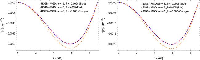
Figure 1. Variation of deformation function f(r) w.r.t. radial coordinate r for compact stars named LMCX-4 (left) and EXO1785-248 (right). |
In the following subsections, we discuss TFS exact solution and its minimally deformed counterpart, where we rename ϵ, Pr and P⊥ as follows
$\begin{eqnarray}{\rho }^{({\rm{t}}{\rm{o}}{\rm{t}})}=8\pi \varepsilon =8\pi (\rho +\beta {\theta }_{0}^{0}),\end{eqnarray}$
$\begin{eqnarray}{p}_{{\rm{r}}}^{({\rm{t}}{\rm{o}}{\rm{t}})}=8\pi {P}_{{\rm{r}}}=8\pi ({p}_{{\rm{r}}}-\beta {\theta }_{1}^{1}),\end{eqnarray}$
$\begin{eqnarray}{p}_{{\rm{t}}}^{({\rm{t}}{\rm{o}}{\rm{t}})}=8\pi {P}_{\perp }=8\pi ({p}_{{\rm{t}}}-\beta {\theta }_{2}^{2}).\end{eqnarray}$
5.1. EGB case
Here we will discuss the variation of physical stellar variables for the case of EGB gravity i.e., β = 0. The variations of energy density ρ(tot) are given in figure 2, which are totally in agreement with the physically accepted trend, i.e., maximum at the center and possess monotonically decreasing behavior towards the surface. The variation of radial pressure ${{p}_{{\rm{r}}}}^{({\rm{t}}{\rm{o}}{\rm{t}})}$ and transverse pressure ${{{\rm{p}}}_{{\rm{t}}}}^{({\rm{t}}o{\rm{t}})}$ is illustrated in figure 3, where cyan and green curves describe the behavior of pressure components in EGB gravity theory. As can be seen, these variations are obtained by using two different values of α = 45 and α = 48. It is observed that radial pressure decreases towards the boundary of stellar objects and vanishes at the boundary of the star. Similarly, transverse pressure decreases towards the boundary but it behaves slightly differently at the surface of the compact star for α = 45 as depicted in figure 3 (left panels). Moreover, the anisotropic factor Δ(tot) (see figure 4) shows the expected behavior for a stellar structure as it is positive throughout the stellar interior. This situation indicates the repulsive nature of anisotropic source which adds to the stability of the system by neutralizing the effects of gravitational force.
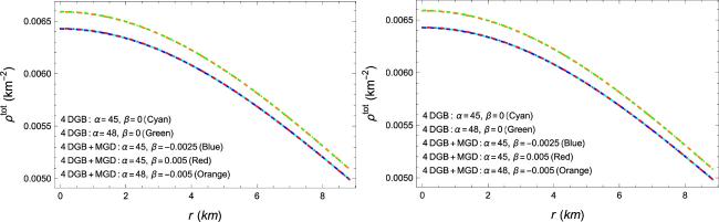
Figure 2. Variation of energy density (ρtot) w.r.t. radial coordinate r of compact stars named LMCX − 4 (left) and EXO1785 − 248 (right). |
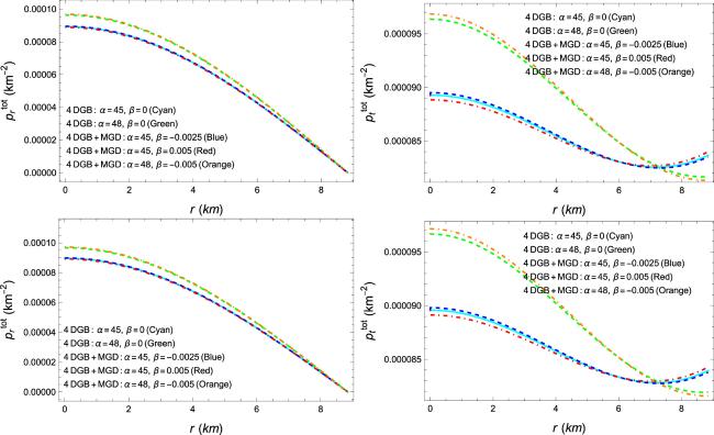
Figure 3. Variation of radial pressure (${{p}}_{{\rm{r}}}^{{\rm{t}}{\rm{o}}{\rm{t}}}$) and tangential pressure (${p}_{{\rm{t}}}^{{\rm{t}}{\rm{o}}{\rm{t}}}$) w.r.t. radial coordinate r of compact stars named LMCX − 4 (upper row) and EXO1785 − 248 (lower row). |
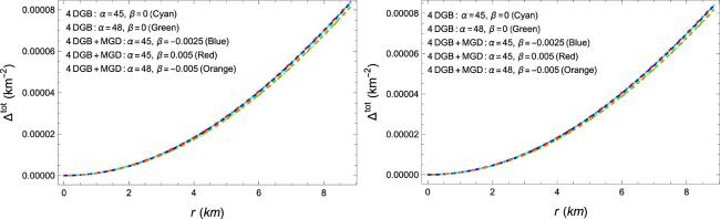
Figure 4. Variation of anisotropic factor (Δtot) w.r.t. radial coordinate r for compact stars named LMCX − 4 (left panel) and EXO1785 − 248 (right panel). |
5.2. EGB+MGD case
The deformation functions h(r) and f(r), given in equations (19 ) and (20 ), control the radial and temporal geometric deformations. For the MGD approach, we set h(r) = 0 which means that the modification of anisotropic solutions fully depends on the radial deformation function f(r), and the temporal metric function remains unaltered. Since, physical quantities such as tangential and radial pressures, energy density, and the mass of compact objects depend on the radial metric potential will also undergo a change.
1: The total energy density ${\rho }^{(\mathrm{tot})}=\rho +\beta {\theta }_{0}^{0}$ also undergoes a change with the addition of an anisotropic source which clearly depends on the β and anisotropic source ${\theta }_{0}^{0}$. However, the variation of anisotropic source ${\theta }_{0}^{0}$ can be entirely traced by observing the behavior of metric potential function μ(r), decoupling function f(r) along with their first derivatives as in equation (25 ). For the under observation mimicking constraint ${p}_{{\rm{r}}}={\theta }_{1}^{1}$, the deformation functions are described in figure 1. The figure shows an interesting behavior of f(r) i.e. f(r) becomes null at the center (i.e. r = 0) and on the boundary (i.e. r = R) of the compact entity. In figure 2, it can be observed that we get more compact objects for positive values of β.
2: By keeping the EGB coupling constant α same and varying the MGD decoupling constant β i.e α = 45, β = 0.005 and β = − 0.0025, one can observe from figure 3 that ${{p}_{{\rm{r}}}}^{({\rm{t}}{\rm{o}}{\rm{t}})}$ shows physically accepted behavior for different values of β, whereas the behavior of ${{{p}}_{{\rm{t}}}}^{({\rm{t}}{\rm{o}}{\rm{t}})}$ slightly disturbs near the boundary. It remains continuous, but it exhibits behavior that deviates from regular trends for certain values of α and β. Usually, the tangential pressure follows a standard trend, i.e., it is maximum at the center and decreases monotonically towards the boundary. However, for specific combinations of α and β, this trend changes near the boundary, leading to a departure from the usual monotonic decrease. It occurs because for certain values of α, higher-order effects produced by the additional curvature corrections, become more significant and have a disproportionate impact on the tangential pressure. By increasing the magnitude of α, the observations are made and it was found that both quantities take greater values at the core of the stellar entity. In this case, ${{p}_{{\rm{r}}}}^{({\rm{t}}{\rm{o}}{\rm{t}})}$ and ${{p}_{{\rm{t}}}}^{({\rm{t}}{\rm{o}}{\rm{t}})}$ show regular trends throughout in the stellar interior.
3: The behavior of anisotropic factor ${\Delta }^{(\mathrm{tot})}\,=8\pi ({p}_{{\rm{t}}}^{(\mathrm{tot})}-{p}_{{\rm{r}}}^{(\mathrm{tot})})$ is illustrated in figure 4 which shows positive anisotropy measure throughout in the stellar interior. Further, it is noted that anisotropy is higher when α = 45 and lower for α = 48, on the other hand, it increases for positive values of β and decreases for negative values of β. The external gravitational source modifies the existing anisotropies within the observed stellar system. These anisotropies in the stellar interior enhance compactness and stability, contributing to the prevention of gravitational collapse for specific choices of parameters.
4: In standard General Relativity, the mass function is derived from the metric potential by solving Einstein's field equations. In the MGD approach, the deformation function f(r) of the radial metric potential modifies the spacetime structure, influencing the total energy-momentum content. This modification can be seen as generating additional mass or, in some cases, negative mass, depending on the sign of f(r). If f(r) is negative, it leads to a reduction in the effective mass of the system, weakening the gravitational field. In extreme cases, this reduction can give rise to negative mass, resulting in repulsive gravitational behavior instead of attraction. Such a reduction in mass can significantly alter the gravitational field, especially near the boundary of the object. However, the effects of the deformation function are controlled by the parameter β, which regulates the degree of deformation. By choosing appropriate values of β, the issue of the negative sign of f(r) can be managed, allowing for a controlled adjustment of the mass generation process. The total mass of the compact object in EGB gravity can be directly calculated by integrating the field equation that incorporates density. Now, using equation (21 ) 25 ). Thus, we have 63 ) and (63 ) as follows
$\begin{eqnarray}{M}_{\mathrm{EGB}}(R)\equiv 4\pi {\int }_{0}^{R}{r}^{2}\rho (r){\rm{d}}r.\end{eqnarray}$
The mass of the object is modified again when EGB gravity is decoupled using the MGD approach, as can be calculated from equation ( $\begin{eqnarray}{M}_{\mathrm{MGD}}(R)\equiv 4\pi {\int }_{0}^{R}{r}^{2}{\theta }_{0}^{0}(r){\rm{d}}r.\end{eqnarray}$
The total mass of the object can be evaluated by adding both masses given in equations ( $\begin{eqnarray}M(R)={M}_{\mathrm{EGB}}(R)+{M}_{\mathrm{MGD}}(R).\end{eqnarray}$
Figure 5 displays the variations in the mass function (left panel) and the mass-radius ratio (right panel). It is observed that both functions attain higher values for α = 48 and lower values for α = 45. However, the influence of the decoupling parameter β on these variations is relatively insignificant.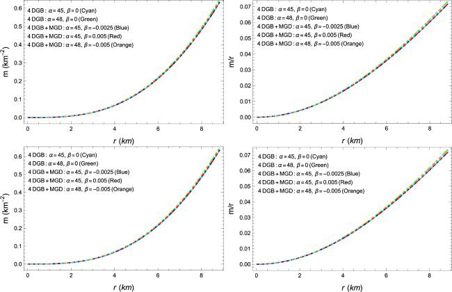
Figure 5. Variation of mass–radius relation m(r) and mass–radius ratio w.r.t. radial coordinate r for compact stars named LMCX − 4 (upper row) and EXO1785 − 248 (lower row). |
6. Energy conditions
The physical properties known as energy conditions are essential for studying actual scenarios related to matter configurations. These constraints reflect the micro-scale characteristics of matter and play a critical role in distinguishing between the usual and unusual properties of matter in the stellar models. They are widely recognized for their applicability in addressing various cosmological issues. Energy conditions are categorized into four types: null energy condition (NEC), weak energy condition (WEC), strong energy condition (SEC), and dominant energy condition (DEC). These conditions are considered satisfied when the specified limits are uniformly met throughout the entire sphere. Mathematically, the conditions are expressed in the following forms
NEC: ${\rho }^{({\rm{t}}{\rm{o}}{\rm{t}})}+{p}_{{\rm{r}}}^{({\rm{t}}{\rm{o}}{\rm{t}})}\geqslant 0$, ${\rho }^{({\rm{t}}{\rm{o}}{\rm{t}})}+{p}_{{\rm{t}}}^{({\rm{t}}{\rm{o}}{\rm{t}})}\geqslant 0$
WEC: ρ(tot)≥0, ${\rho }^{({\rm{t}}{\rm{o}}{\rm{t}})}+{p}_{{\rm{r}}}^{({\rm{t}}{\rm{o}}{\rm{t}})}\geqslant 0$ and ${\rho }^{({\rm{t}}{\rm{o}}{\rm{t}})}+{p}_{{\rm{t}}}^{({\rm{t}}{\rm{o}}{\rm{t}})}\geqslant 0$
SEC: ${\rho }^{({\rm{t}}{\rm{o}}{\rm{t}})}+{p}_{{\rm{r}}}^{({\rm{t}}{\rm{o}}{\rm{t}})}+2{p}_{{\rm{t}}}^{({\rm{t}}{\rm{o}}{\rm{t}})}\geqslant 0$
DEC: ${\rho }^{({\rm{t}}{\rm{o}}{\rm{t}})}-{p}_{{\rm{t}}}^{({\rm{t}}{\rm{o}}{\rm{t}})}\geqslant 0$ and ${\rho }^{({\rm{t}}{\rm{o}}{\rm{t}})}-{p}_{{\rm{r}}}^{({\rm{t}}{\rm{o}}{\rm{t}})}\geqslant 0$
As illustrated in figures 2 and 3, NEC, WEC, and SEC are satisfied for the studied configurations. These findings show that the matter distributions in the models meet the fundamental energy conditions necessary for the stability and viability of the stellar structures. The behavior of DEC is presented in figure 6. This figure highlights the fulfillment of the DEC for the stars considered in this study. The DEC is crucial for ensuring that the energy density is high enough for meaningful physical scenarios, confirming that the stellar models maintain the necessary energy conditions throughout their interiors.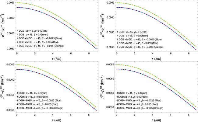
Figure 6. Variation of dominant energy conditions w.r.t. radial coordinate r for compact stars named as LMCX − 4 (upper row) and EXO1785 − 248 (lower row). |
7. Square sound speeds and Herrera's cracking condition
The perseverance of causality condition demands that the sound speed should not exceed the speed of light, where the components of sound speed in radial and transverse direction, denoted by ${V}_{{\rm{t}}}^{2}$ and ${V}_{{\rm{r}}}^{2}$ respectively, are defined as
$\begin{eqnarray}{V}_{{\rm{r}}}^{2}=\displaystyle \frac{{\rm{d}}{p}_{{\rm{r}}}^{\mathrm{tot}}}{{\rm{d}}{\rho }^{\mathrm{tot}}},\quad {V}_{{\rm{t}}}^{2}=\displaystyle \frac{{\rm{d}}{p}_{{\rm{t}}}^{\mathrm{tot}}}{{\rm{d}}{\rho }^{\mathrm{tot}}}.\end{eqnarray}$
For a physically viable model of an anisotropic fluid sphere, both the radial and transverse components of the sound speed should be less than 1. The left panels of figure 7 show the variation of the radial component, which satisfies the causality condition for both stars. The right panels illustrate that the transverse component meets the condition over a large domain; however, it becomes negative near the boundary for α = 45. In addition to the causality condition, Herrera and his collaborators proposed the 'cracking' concept, which states that a region is stable if $0\leqslant | {V}_{{\rm{r}}}^{2}-{V}_{{\rm{t}}}^{2}| \leqslant 1$. As seen in figure 7, the modulus value of ${V}_{{\rm{r}}}^{2}-{V}_{{\rm{t}}}^{2}$ consistently falls within this range, confirming that no cracking occurs in the compact model.
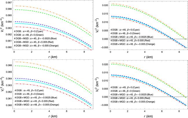
Figure 7. Variation of speed of sound ${V}_{{\rm{r}}}^{2}$ and ${V}_{{\rm{t}}}^{2}$ w.r.t. radial coordinate r for compact stars named as LMCX − 4 (upper row) and EXO1785 − 248 (lower row). |
8. TOV equation
Compact stars are astrophysically expected to be in an equilibrium state. The Tolman–Oppenheimer–Volkoff (TOV) equation serves as a fundamental tool to analyze the equilibrium of such compact systems. This equation states that the sum of all forces acting on the system must be zero for it to remain in equilibrium. In the present study, the TOV equation is expressed in equation (16 ), where we can identify the contributing forces explicitly as follows
$\begin{eqnarray}{F}_{{\rm{h}}}={p}_{{\rm{r}}}^{{\prime} }-\beta ({\theta }_{1}^{1})^{\prime} ,\end{eqnarray}$
$\begin{eqnarray}{F}_{{\rm{g}}}=(\rho +{p}_{{\rm{r}}})\phi ^{\prime} +\beta \phi ^{\prime} ({\theta }_{0}^{0}-{\theta }_{1}^{1}),\end{eqnarray}$
$\begin{eqnarray}{F}_{{\rm{a}}}=\frac{2}{{\rm{r}}}({p}_{{\rm{r}}}-{p}_{{\rm{t}}})-\frac{3}{{\rm{r}}}\beta ({\theta }_{1}^{1}-{\theta }_{2}^{2}),\end{eqnarray}$
where Fh, Fg and Fa are known as hydrostatic, gravitational and anisotropic forces, respectively. Here, the total sum of all the mentioned forces must be zero, i.e., $\begin{eqnarray}{F}_{h}+{F}_{g}+{F}_{a}=0.\end{eqnarray}$
The evolution of above described forces can be seen in figure 8. It can be observed that the hydrostatic and anisotropic forces have positive values, while the gravitational force is negative. This indicates that the outward-directed hydrostatic and anisotropic forces are counterbalanced by the inward-directed gravitational force, maintaining equilibrium within the system.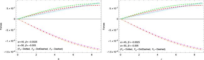
Figure 8. Evolution of forces w.r.t. radial coordinate r for compact stars named as LMCX − 4 (left panel) and EXO1785 − 248 (right panel). |
9. Adiabatic index
The adiabatic index serves as a crucial tool for assessing the stability of stellar models. For a static, spherically symmetric stellar model to be stable, the value of the adiabatic index must be greater than $\frac{3}{4}$. The radial and tangential adiabatic indices, which provide insights into the stability against radial perturbations, are defined by the following mathematical expressions
$\begin{eqnarray}{{\rm{\Gamma }}}_{{\rm{r}}}=\frac{{\rm{d}}(\mathrm{log}{p}_{{\rm{r}}}^{{\rm{t}}{\rm{o}}{\rm{t}}})}{{\rm{d}}(\mathrm{log}{\rho }^{{\rm{t}}{\rm{o}}{\rm{t}}})},\quad {{\rm{\Gamma }}}_{{\rm{t}}}=\frac{{\rm{d}}(\mathrm{log}{p}_{{\rm{t}}}^{{\rm{t}}{\rm{o}}{\rm{t}}})}{{\rm{d}}(\mathrm{log}{\rho }^{{\rm{t}}{\rm{o}}{\rm{t}}})},\end{eqnarray}$
However, we will focus on the radial component since gravitational collapse primarily occurs along the radial direction. Figure 9 illustrates the behavior of the radial adiabatic index, Γr. It is evident that Γr consistently exceeds the value of $\frac{4}{3}$, satisfying the stability criterion required for the model. On the other hand, the critical adiabatic index is defined as $\begin{eqnarray}{{\rm{\Gamma }}}_{\,\rm{critical}\,}=\frac{4}{3}+\frac{19}{21}u,\quad \,\rm{with}\,\quad u=\frac{M}{R}.\end{eqnarray}$
For stable stellar configuration, adiabatic index and critical adiabatic index should satisfy the inequality, given by Γr ≥ Γcritical. The bottom panel of figure 9 shows the variation of Γcritical, which is clearly in accordance with the aforementioned relation between Γr and Γcritical.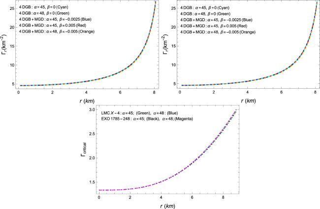
Figure 9. Evaluation of adiabatic index Γr for compact stars named LMCX − 4 (left panel) and EXO1785 − 248 (right panel) and critical adiabatic index Γcritical (bottom panel) w.r.t. radial coordinate r for both stars. |
10. Concluding remarks
The study of self-gravitating compact objects such as NSs, white dwarfs, and black holes is crucial for advancing theoretical physics, especially when it comes to understanding the Universe under extreme conditions. Investigating these objects is essential for constructing physically realistic and mathematically rigorous anisotropic solutions. Due to their intense gravitational fields, these compact stars serve as natural laboratories for testing the viability of various gravitational theories and exploring the fundamental properties of matter in high-density environments. In this article, we present a comprehensive model to investigate the anisotropic structure of stellar objects in the framework of EGB gravity theory. This gravitational theory is notable for avoiding ghost instabilities, which can lead to undesirable irregularities in theoretical models.
We have considered a novel MGD approach to address the complexities of the presented model. This approach effectively separates the internal anisotropic matter from the externally imposed anisotropy through gravitational means. Specifically, the MGD technique modifies only the radial metric potential while keeping the temporal component unchanged. Moreover, this approach enables the decoupling of the gravitational source from the combined system of field equations into two distinct parts: one representing an anisotropic source corresponding to the standard system of field equations in EGB gravity, while the other consisting of the quasi-Einstein field equations associated with an external gravitational source. We achieve the desired results by solving the standard system using the known TFS anisotropic solution. On the other hand, the quasi-Einstein system of field equations is closed by applying a pressure-mimicking constraint, ${p}_{{\rm{r}}}={\theta }_{1}^{1}$.
A vital part of our findings is the matching of TFS inner spacetime with Bolware–Deser outer spacetime, guaranteeing the smooth transition between the internal and external spacetime solutions. This matching is crucial for the mathematical reliability and physical feasibility of the stellar structure. The thermodynamic properties of the stellar model are thoroughly examined, focusing on the total energy density (ρtot), total radial pressure (${p}_{{\rm{r}}}^{{\rm{t}}{\rm{o}}{\rm{t}}}$) and total tangential pressure (${p}_{{\rm{t}}}^{{\rm{t}}{\rm{o}}{\rm{t}}}$). The evolution of total energy density (ρtot) is observed to be positive throughout the inner stellar distribution, reaching its maximum at the core of the compact star. Similarly, total radial pressure (${p}_{{\rm{r}}}^{{\rm{t}}{\rm{o}}{\rm{t}}}$) and total tangential pressure (${p}_{{\rm{t}}}^{{\rm{t}}{\rm{o}}{\rm{t}}}$) also demonstrate positive values within the stellar distribution, attaining their highest values at the star's core. The first two quantities exhibit regular and continuous behavior for all the selected parameters. However the total tangential pressure remains continuous, but it shows deviations from the expected trends near the boundary for certain values of α and β.
Moreover, the anisotropy factor of the stellar structure is scrutinized. The anisotropic factor in figure 4 remains positive throughout the stellar interior. The anisotropy is more pronounced at α = 45 compared to α = 48, and it increases with positive values of β while decreasing with negative values. The external gravitational source influences the existing anisotropies within the stellar system. We thoroughly examined the stability of the stellar model by imposing causality condition and Herrera's cracking criterion. Since there is no sign change in the term ${V}_{{\rm{r}}}^{2}-{V}_{{\rm{t}}}^{2}$, acting as the stability indicator, affirms that there is no cracking in the model. The examination of the energy conditions, the TOV equation, and the adiabatic index further reinforces the physical stability of the stellar model.
In conclusion, this work not only develops our understanding of anisotropic structures in the field of compact stars through a novel model within EGB gravity but also demonstrates that MGD technique facilitates precise and physically meaningful solutions. The analyses provide valuable insights into the physical properties and stability of these stellar models, enriching our understanding of theoretical physics and opening new avenues for future research in modified gravitational theories and the modeling of compact objects.