Amjad Hussain, Ayesha Almas, M Farasat Shamir, Adnan Malik, Sajjad Shaukat Jamal. Charged stellar structures with Adler–Finch–Skea geometry in Ricci-inverse gravity[J]. Communications in Theoretical Physics, 2025, 77(6): 065402. DOI: 10.1088/1572-9494/ad9c3f
1. Introduction
Dark energy and dark matter are two of the most mysterious components of the Universe. Dark matter, which makes up about 27% of the Universe, does not emit, absorb, or reflect light, yet its gravitational effects are essential for explaining the rotation of galaxies and large-scale structure formation. Dark energy, on the other hand, accounts for roughly 68% of the Universe and is thought to be responsible for the accelerated expansion of the cosmos. Together, these components dominate the Universe's mass-energy content, yet their true nature remains largely unknown [1]. While general relativity (GR) has been remarkably successful in describing gravitational phenomena, it falls short in explaining the accelerating expansion of the Universe, as well as the behavior of dark matter and dark energy [2–4]. Modified theories of gravity aim to extend GR by incorporating additional degrees of freedom and higher-order corrections into the field equations. These extensions allow for a more comprehensive framework that can address phenomena that is unexplained by GR, offering deeper insights into the evolution of the Universe, especially in the context of dark energy and dark matter. Modified theories of gravity provides a promising pathway to bridge the gap between observed cosmic behavior and our theoretical understanding of gravity. Some of these modified theories of gravity are f(R), f(G), f(Q),f(T), f(R, T), f(G, T), f(R, G), f(R, φ) and f(R, φ, X) [5–26, 113] theories of gravity. Recently, Celine [27] discussed a new theory of modified gravity that appears to be a novel alternative to particle dark matter. Capozziello et al, [28] investigated the evolution of the Universe at infrared scales as an Infinite Derivative Gravity model of the Ricci scalar, without introducing the cosmological constant or any scalar field. Das et al, [29] considered the stellar object filled by a mixture of two non-interacting isotropic ordinary matter and anisotropic dark energy in the fluid state, named by dark energy star and investigated a stable spherically symmetric relativistic stellar configuration. Goswami and Das [30] proposed a simple parametrization for the pressure component p(z) of the dark energy model and have studied the cosmological implications of this model in the framework of f(Q) modified gravity theory.
The $f({ \mathcal R },{ \mathcal A })$ modified theory of gravity is an extension of GR that incorporates both the Ricci scalar $({ \mathcal R })$ and the antisymmetric curvature scalar $({ \mathcal A })$ to better describe gravitational interactions. In standard GR, gravity is explained solely through the curvature of spacetime, represented by the Ricci scalar. However, this framework struggles to fully explain phenomena such as dark energy, dark matter, and the accelerated expansion of the Universe. By introducing an additional dependence on the anti-curvature scalar $({ \mathcal A })$, the $f({ \mathcal R },{ \mathcal A })$ theory allows for more flexibility in modeling the universes large-scale behavior. This coupling between $({ \mathcal R })$ and $({ \mathcal A })$ adds extra degrees of freedom, which can account for modifications in gravitational dynamics, particularly in strong-field regimes or at cosmic scales. As a result, $f({ \mathcal R },{ \mathcal A })$ theories have the potential to provide new insights into the nature of dark energy, the early universe, and the formation of compact objects, offering a more complete gravitational framework than GR. Das et al [31] proposed a geometrical theory of gravity containing higher-order derivative terms and introduced anti-curvature scalar, which is the trace of the inverse of the Ricci tensor. Recently, Malik et al [32] used the Karmarkar condition to investigate the charged anisotropic characteristics of compact stars in modified Ricci-inverse gravity. Shamir along with his collaborators [33] investigated the quintessence compact relativistic spherically symmetrical anisotropic solutions under the recently developed Ricci-inverse gravity by employing Krori and Barua gravitational potentials. Jawad and Malik [33, 34] investigated the matter-antimatter asymmetry through baryogenesis (and generalized gravitational baryogenesis interaction) in the realm Ricci-inverse gravity. Do [35] studied the so-called Ricci-inverse gravity, which is a very novel type of fourth-order gravity and figured out both isotropically and anisotropically inflating universes to this model. Malik et al [36] conducted an extensive investigation of stellar compact structures within the frame of the newly proposed Ricci-inverse theory of gravity by utilizing the Tolman–Kuchowicz spacetime. de Souza and Santos [37] introduced into the Einstein–Hilbert action an anti-curvature scalar that is obtained from the anti-curvature tensor which is the inverse of the Ricci tensor and studied an axially symmetric spacetime with causality violation. Recently, Malik with his collaborators [38] explored wormhole solutions by analyzing energy conditions within the framework of $f({ \mathcal R },{ \mathcal A })$ modified theory of gravity. They [39] also presented the charged wormhole solutions within the framework of modified $f({ \mathcal R },{ \mathcal A })$ gravity by taking into account the charged anisotropic matter composition and Karmarkar condition.
Understanding the behavior of pressure in spherically symmetric stellar models is crucial, as pressure within compact objects may vary in different directions. In these models, pressure can be divided into two components: radial pressure pr, and transverse pressure pt, with pt acting perpendicular to pr. The difference between these pressures, known as the anisotropic factor Δ, is defined as Δ = pt − pr. Anisotropy is introduced based on observations that in the high-density environments of compact stars, the radial and transverse pressures differ, as noted by Canuto [40]. Ruderman's theoretical work [41] showed that compact objects tend to become anisotropic at extremely high densities, approximately 1015g/cm3. Kippenhahn and Weigert [42] proposed that anisotropy in relativistic stars could be due to the presence of a solid core or a type-III A superfluid within the star. Furthermore, Weber [43] demonstrated that strong magnetic fields in dense stars result in non-uniform pressure in different directions. Anisotropy can also arise from other factors, including viscosity, phase transitions [44], pion condensation [45], and even fluid shear in self-gravitating objects [46]. Mak and Herko [47] developed exact solutions to the Einstein field equations for spherically symmetric anisotropic stars, while Petri [48] derived an exact solution for compact objects with locally anisotropic pressure. Ivanov [49] established a surface redshift limit for realistic anisotropic stars. Recent studies [50–61] continue to explore the structure and effects of pressure anisotropy in compact stars. Investigating these objects in higher-dimensional frameworks is particularly intriguing. For instance, Takisa and Maharaj [62] used a linear equation of state to derive solutions for anisotropic, spherically symmetric, charged distributions.
In this study, the Finch–Skea metric potential is employed to investigate compact objects within the framework of $f({ \mathcal R },{ \mathcal A })$ gravity. Finch and Skea [63] introduced a realistic stellar model aimed at improving upon the Dourah and Ray [64] metric, which was not suitable for describing ultra-compact objects. The Finch–Skea ansatz has since become widely used in the development of realistic stellar models, as referenced by various researchers [65, 66]. This metric is considered particularly well-suited for studying compact stars, as it satisfies the conditions for perfect fluid matter [67]. Kalam et al [68, 69] utilized the Finch–Skea metric to model strange quark stars, incorporating the MIT bag model and two-fluid models. Their work extended the metric by introducing anisotropic pressure corresponding to normal matter to propose models of quintessence stars [70]. Maharaj et al [71] further generalized the Finch–Skea geometry by including charge and anisotropy, demonstrating the potential for modeling more complex stellar configurations. Kileba et al [72] examined different scenarios charged with anisotropy, charged with isotropy, and isotropic without charge and found that these models align well with several observed compact stars. Bhar et al [73] applied the Finch–Skea metric in (2 + 1) dimensions to produce anisotropic stars, while Shamir et al [74] explored compact geometries using the Finch–Skea metric and the Karmarkar condition in the presence of charged anisotropic matter distributions. Moreover, several researchers [75–92] have extended the study of the stellar structures to higher-dimensional spaces, further expanding its applicability in theoretical astrophysics.
This study aims to investigate the physical properties of a spherically symmetric and anisotropic compact star model in higher dimensions, incorporating the limitations of Finch–Skea geometry. This paper significantly contributes to the understanding of spherically symmetric solutions in modified gravity by introducing a novel class of charged, anisotropic models characterized by the function f(R, A) = R + αA. By utilizing the modified Ricci-inverse gravity framework, the study addresses the complexities of modeling compact objects, which are often overlooked in traditional homogeneous spaces. Key findings include the regularity of metric potentials and the satisfaction of energy conditions, highlighting the stability and physical viability of the proposed models. This work not only advances theoretical insights into the structure and dynamics of compact stars but also establishes a comprehensive analytical approach for exploring their characteristics in the context of modified gravity, thereby bridging the gap between classical and contemporary astrophysical models. Our paper is structured as follows: section 2 deals with some basic formulism of Ricci-inverse gravity. The detailed overview of Karmarkar condition is provided in section 3. Section 4 outlines the methodology for determining the unknown parameters present in the metric potentials by aligning the interior spacetime with the exterior Bardeen spacetime. Section 5 deals with the detailed graphical analysis of various physical characteristics of the stars, such as energy density, radial and tangential pressure, anisotropy, energy conditions, equation of state parameters, mass function, compactness factor, redshift function and stability analysis. The Appendix summarizes our findings.
2. Basic formalism of Ricci-inverse gravity
This section summarizes the key concepts of modified Ricci-inverse gravity, a newly proposed alternative theory of gravity. In this framework, the inverse of the Ricci tensor ${{ \mathcal R }}_{\xi \sigma }$ is named as the anti-curvature tensor ${{ \mathcal A }}^{\xi \sigma }$. Mathematically, the anti-curvature tensor and the Ricci tensor have the following relationship:
$\begin{eqnarray}{{ \mathcal A }}^{\eta \xi }{{ \mathcal R }}_{\xi \sigma }={\delta }_{\sigma }^{\eta },\end{eqnarray}$
where the term ${\delta }_{\sigma }^{\eta }$ is called Kronecker delta. Based on the anti-curvature tensor, the anti-curvature scalar ${ \mathcal A }$ is defined as
$\begin{eqnarray}{ \mathcal A }={g}_{\eta \xi }{{ \mathcal A }}^{\eta \xi }.\end{eqnarray}$
It is important to note that ${ \mathcal A }$ is not simply the inverse of ${ \mathcal R }$. The action of ${ \mathcal R }$ and ${ \mathcal A }$ gravity is defined as
$\begin{eqnarray}S=\int {{\rm{d}}}^{4}x\sqrt{-g}\left(f({ \mathcal R },{ \mathcal A })+{{ \mathcal L }}_{m}+{{ \mathcal L }}_{{\rm{e}}}\right),\end{eqnarray}$
where g is the determinant of the metric tensor, while ${{ \mathcal L }}_{m}$ and ${{ \mathcal L }}_{{\rm{e}}}$ denote the Lagrangian components corresponding to matter and electric field, respectively. We can get the field equations by varying the action (3) with respect to the metric tensor as
$\begin{eqnarray}\begin{array}{rcl}{f}_{{ \mathcal R }}{{ \mathcal R }}^{\eta \xi }-{f}_{{ \mathcal A }}{{ \mathcal A }}^{\eta \xi } & - & \frac{1}{2}f{g}^{\eta \xi }+{g}^{\rho \eta }{{\rm{\nabla }}}_{\omega }{{\rm{\nabla }}}_{\rho }{f}_{{ \mathcal A }}{{ \mathcal A }}_{\sigma }^{\omega }{{ \mathcal A }}^{\xi \sigma }\\ & - & \frac{1}{2}{{\rm{\nabla }}}^{2}({f}_{{ \mathcal A }}{{ \mathcal A }}_{\sigma }^{\eta }{{ \mathcal A }}^{\xi \sigma })\\ & - & \frac{1}{2}{g}^{\eta \xi }{{\rm{\nabla }}}_{\omega }{{\rm{\nabla }}}_{\beta }({f}_{{ \mathcal A }}{{ \mathcal A }}_{\sigma }^{\omega }{{ \mathcal A }}^{\beta \sigma })\\ & - & {{\rm{\nabla }}}^{\eta }{{\rm{\nabla }}}^{\xi }{f}_{{ \mathcal R }}+{g}^{\eta \xi }{\rm{\nabla }}{f}_{{ \mathcal R }}={{ \mathcal T }}^{\eta \xi },\end{array}\end{eqnarray}$
where the term ${f}_{{ \mathcal R }}=\frac{\partial f}{\partial { \mathcal R }}$, ${f}_{{ \mathcal A }}=\frac{\partial f}{\partial { \mathcal A }}$, ∇α represents covariant derivative, and ∇ = ∇η∇η is the d'Alembert operator. Moreover, the covariant divergence of the equation (4) yields the following equation as
$\begin{eqnarray}\begin{array}{rcl}{{\rm{\nabla }}}_{\eta }{{ \mathcal T }}^{\eta \xi } & = & -\frac{1}{2}{g}^{\eta \xi }{f}_{{ \mathcal A }}{{\rm{\nabla }}}_{\eta }{ \mathcal A }-{{\rm{\nabla }}}_{\eta }({f}_{{ \mathcal A }}{{ \mathcal A }}^{\eta \xi })\\ & & +{g}^{\rho \eta }{{\rm{\nabla }}}_{\eta }\left[\right.{{\rm{\nabla }}}_{\omega }{{\rm{\nabla }}}_{\rho }({f}_{{ \mathcal A }}{{ \mathcal A }}_{\sigma }^{\omega }{{ \mathcal A }}^{\xi \sigma })\left]\right.\\ & & -\frac{1}{2}{{\rm{\nabla }}}_{\eta }\left[\right.{{\rm{\nabla }}}^{2}({f}_{{ \mathcal A }}{{ \mathcal A }}_{\sigma }^{\eta }{{ \mathcal A }}^{\xi \sigma })\left]\right.\\ & & -\frac{1}{2}{g}^{\eta \xi }{{\rm{\nabla }}}_{\eta }\left[\right.{{\rm{\nabla }}}_{\omega }{{\rm{\nabla }}}_{\beta }({f}_{{ \mathcal A }}{{ \mathcal A }}_{\sigma }^{\omega }{{ \mathcal A }}^{\beta \sigma })\left]\right..\end{array}\end{eqnarray}$
For our current work, we consider the simplest linear model for $f({ \mathcal R },{ \mathcal A })$ gravity, which is defined as
$\begin{eqnarray}f({ \mathcal R },{ \mathcal A })={ \mathcal R }+\alpha { \mathcal A }.\end{eqnarray}$
After some manipulation of equations (4), (5) and (6), we get
$\begin{eqnarray}\begin{array}{rcl}{{ \mathcal R }}^{\eta \xi } & - & \frac{1}{2}{ \mathcal R }{g}^{\eta \xi }-\alpha {{ \mathcal A }}^{\eta \xi }-\frac{1}{2}\alpha { \mathcal A }{g}^{\eta \xi }+\frac{\alpha }{2}\left[2{g}^{\rho \eta }{{\rm{\nabla }}}_{\omega }{{\rm{\nabla }}}_{\rho }{{ \mathcal A }}_{\sigma }^{\omega }{{ \mathcal A }}^{\xi \sigma }\right.\\ & - & \left.{{\rm{\nabla }}}^{2}{{ \mathcal A }}_{\sigma }^{\eta }{{ \mathcal A }}^{\xi \sigma }-{g}^{\eta \xi }{{\rm{\nabla }}}_{\omega }{{\rm{\nabla }}}_{\beta }{{ \mathcal A }}_{\sigma }^{\omega }{{ \mathcal A }}^{\beta \sigma }\right]={{ \mathcal T }}^{\eta \xi },\end{array}\end{eqnarray}$
$\begin{eqnarray}\begin{array}{rcl}{{\rm{\nabla }}}_{\eta }{{ \mathcal T }}^{\eta \xi } & = & -\frac{\alpha }{2}{g}^{\eta \xi }{{\rm{\nabla }}}_{\eta }{ \mathcal A }-\alpha {{\rm{\nabla }}}_{\eta }({{ \mathcal A }}^{\eta \xi })\\ & & +\alpha {g}^{\rho \eta }{{\rm{\nabla }}}_{\eta }\left[\right.{{\rm{\nabla }}}_{\omega }{{\rm{\nabla }}}_{\rho }({{ \mathcal A }}_{\sigma }^{\omega }{{ \mathcal A }}^{\xi \sigma })\left]\right.\\ & & -\frac{\alpha }{2}{{\rm{\nabla }}}_{\eta }\left[\right.{{\rm{\nabla }}}^{2}({{ \mathcal A }}_{\sigma }^{\eta }{{ \mathcal A }}^{\xi \sigma })\left]\right.\\ & & -\frac{\alpha }{2}{g}^{\eta \xi }{{\rm{\nabla }}}_{\eta }\left[\right.{{\rm{\nabla }}}_{\omega }{{\rm{\nabla }}}_{\beta }({{ \mathcal A }}_{\sigma }^{\omega }{{ \mathcal A }}^{\beta \sigma })\left]\right..\end{array}\end{eqnarray}$
This work focuses on investigating a static and spherically symmetric matter distribution, where the interior metric is described by the coordinates xμ = (t, r, θ, φ) in the following form as
where ψ and λ represent functions dependent on the radial coordinate r. The spherically symmetric solution presented in this study offers a range of promising applications in both astrophysics and cosmology. Primarily, it serves as a robust framework for modeling the structure and stability of compact stars, such as neutron stars and white dwarfs, where the interplay of charge and anisotropic pressure is crucial. This contributes to a deeper understanding of their formation, evolution, and the fundamental forces in extreme environments. Moreover, the solution is poised to address significant challenges in modified gravity theories, potentially shedding light on the nature of dark matter and dark energy. By incorporating charged anisotropic models, our findings may provide insights into various cosmological phenomena, such as galaxy rotation curves and the dynamics of cosmic structures. Additionally, the framework could facilitate the exploration of gravitational wave emissions from compact objects, enhancing our comprehension of these cosmic events. Overall, we believe that this solution is a valuable tool for addressing a variety of pressing questions in contemporary physics and cosmology, and we appreciate the opportunity to clarify its potential applications. We consider the matter present within the star possesses both charge and anisotropic nature. Consequently, in mixed tensor notation form, the energy-momentum tensor ${{ \mathcal T }}_{\ \xi }^{\eta }$ is considered to be the combination of two components: ${{ \mathcal M }}_{\ \xi }^{\eta }$ for matter contribution and ${{ \mathcal E }}_{\ \xi }^{\eta }$ for electromagnetic contribution, i.e.
$\begin{eqnarray}{{ \mathcal T }}_{\ \xi }^{(\eta )}={{ \mathcal M }}_{\ \xi }^{(\eta )}+{{ \mathcal E }}_{\ \xi }^{(\eta )}.\end{eqnarray}$
In the context of anisotropic fluid with energy density ρ, radial pressure pr, and tangential pressure pt, the energy-momentum tensor for matter represented by ${{ \mathcal M }}_{\ \xi }^{(\eta )}$ is defined as:
Additionally, electromagnetic field tensor ${{ \mathcal E }}_{\ \xi }^{\eta }$ is defined as follows:
$\begin{eqnarray}{{ \mathcal E }}_{\ \xi }^{(\eta )}=-\frac{1}{4\pi }\left[{{ \mathcal F }}^{\eta \gamma }{{ \mathcal F }}_{\xi \gamma }-\frac{1}{4}{\delta }_{\ \xi }^{\eta }{{ \mathcal F }}^{\gamma \chi }{{ \mathcal F }}_{\gamma \chi }\right].\end{eqnarray}$
In equation (11), the fluid's four-velocity, represented as uη, satisfies the normalization condition uηuη = − 1. Similarly, the unit radial four-vector kη adheres to the condition kηkη = 1. The term Δ refers to the anisotropic factor, defined as the difference between the radial pressure and the tangential pressure. Furthermore, in equation (12), ${{ \mathcal F }}_{\eta \xi }$ denotes the electromagnetic field tensor, which can be expressed in terms of the four-potential φη as:
In the study of static spheres, the four-potential φη is generally chosen to take the form (φ(r), 0, 0, 0). As outlined in equation (13), this leads to the presence of non-zero components in the electromagnetic field tensor: ${{ \mathcal F }}_{01}=-{{ \mathcal F }}_{10}=-\varphi ^{\prime} (r)$. The Maxwell equations are given by:
$\begin{eqnarray}\begin{array}{l}\frac{\partial }{\partial {x}^{\gamma }}(\sqrt{-g}{{ \mathcal F }}^{\chi \gamma })=-4\pi \sqrt{-g}{j}^{\chi },\\ {{ \mathcal F }}_{\chi \gamma ,\omega }+{{ \mathcal F }}_{\gamma \omega ,\chi }+{{ \mathcal F }}_{\omega \chi ,\gamma }=0,\end{array}\end{eqnarray}$
where jχ = σuχ is the four-current density vector, where σ represents the proper charge density. In the context of a static matter distribution, the only non-zero component of the four-current is j0, which depends solely on the radial coordinate r due to the system's spherical symmetry. As a result, the non-zero components of the electromagnetic field tensor are ${{ \mathcal F }}^{01}$ and ${{ \mathcal F }}^{10}$, which satisfy the relation ${{ \mathcal F }}^{01}=-{{ \mathcal F }}^{10}$. These components represent the radial component of the electric field. Considering the line element defined in equations (9) and (13), the electromagnetic field equation from equation (14) can be transformed into the following equation:
where the values of ${{ \mathcal R }}^{00}$, ${{ \mathcal R }}^{11}$, ${{ \mathcal R }}^{22}$, ${ \mathcal R }$, ${{ \mathcal A }}^{00}$, ${{ \mathcal A }}^{11}$, ${{ \mathcal A }}^{22}$, ${ \mathcal A }$, ${{ \mathcal A }}_{0}^{0}{{ \mathcal A }}^{00}$, ${{ \mathcal A }}_{1}^{1}{{ \mathcal A }}^{11}$, and ${{ \mathcal A }}_{2}^{2}{{ \mathcal A }}^{22}$ are given in the Appendix.
3. Karmarkar condition
This section deals with the basic formulism of Karmarkar condition. Obtaining an exact solution for the field equations given in equations (21)-(24) is a challenging task due to their non-linear nature. To address this, we construct specific forms of the metric potentials. We utilize a technique developed by Karmarkar, which provides a method to solve the field equations. In this approach, the Riemann curvature tensor ${{ \mathcal R }}_{\xi \alpha \beta \zeta }$ satisfies a specific condition known as the Karmarkar condition [93]. This condition produces an equation that links the two metric components g00 and g11, effectively reducing the problem to a single equation. Consequently, to integrate the field equations, we only need to assume one metric potential and a relation for the electric field intensity. The well-known Karmarkar condition is defined as follows:
with R2323 ≠ 0. A spacetime is classified as belonging to embedding class I if it satisfies the Karmarkar condition, as outlined in equation (25). This condition plays a key role in exploring solutions for astrophysical models. In this study, we utilize the Karmarkar condition to derive a solution for a charged anisotropic model within the framework of Ricci-inverse gravity. Given the line element in equation (9), the non-zero components of the Riemann curvature tensor are:
This metric form of e2λ is similar to that of Finch–Skea solution [103]. The Finch–Skea model that satisfies the Karmarkar condition typically simplifies the analysis by focusing on specific metric potentials without a comprehensive treatment of boundary conditions. While the Finch–Skea approach can yield viable solutions, it may overlook the intricate interplay of physical parameters and the conditions necessary for ensuring a smooth transition between the stellar interior and the external environment. The method employed in this study, therefore, provides a more rigorous framework that not only adheres to Karmarkar's condition but also incorporates detailed boundary conditions, enhancing the physical validity and applicability of the model in real astrophysical scenarios. Consider the electric field in the form given below
$\begin{eqnarray}{E}^{2}=kYr,\end{eqnarray}$
where k is an arbitrary constant. The parameter k in our calculations is an arbitrary value but is carefully chosen based on specific physical requirements within the framework of our model. In the context of our work, k plays a pivotal role in determining the behavior of various physical quantities, such as energy density, pressure components, and the overall stability of the stellar configuration. The value of k is constrained by the need to satisfy essential conditions, including the energy conditions, causality requirements, and the smooth matching of the interior solution to the exterior spacetime at the boundary of the star. Moreover, its selection is informed by ensuring that the solution remains physically viable, stable, and free from singularities within the stellar interior. While the choice of k may vary depending on the specific system under consideration, it is always governed by these physical constraints rather than being arbitrarily selected. We hope this clarification helps, and we are happy to provide further details if needed. Please note that for our current analysis, we consider k = 0.00015. By utilizing the metric potentials defined in equations (28) and (29), we obtain the physical entities as
$\begin{eqnarray}\begin{array}{l}\frac{1}{2}\left[\alpha { \mathcal A }-2\alpha X{{ \mathcal A }}^{00}{\left({r}^{2}Y+1\right)}^{2}-\frac{1}{{\left(16L{r}^{3}X{Y}^{2}+r\right)}^{2}}\right.\\ \left\{\alpha \left(4{r}^{2}XY({{ \mathcal A }}_{0}^{0}{{ \mathcal A }}^{00})\left({r}^{2}Y(1-32LXY)-1\right)-4({{ \mathcal A }}_{1}^{1}{{ \mathcal A }}^{11})\right.\right.\\ \quad \times \,\left(8L{r}^{2}X{Y}^{2}+1\right)\left(32L{r}^{2}X{Y}^{2}+1\right)\\ \quad +\,\,r\left(2X({{ \mathcal A }}_{0}^{0}{{ \mathcal A }}^{00})^{\prime} \left({r}^{2}Y+1\right)\right.\\ \quad \times \,\left({r}^{2}Y\left(8LXY\left(9{r}^{2}Y+1\right)+5\right)+1\right)\\ \quad +\,r\left(16L{r}^{2}X{Y}^{2}+1\right)\left(-48LrX{Y}^{2}({{ \mathcal A }}_{1}^{1}{{ \mathcal A }}^{11})^{\prime} \right.\\ \quad -\,2r({{ \mathcal A }}_{2}^{2}{{ \mathcal A }}^{22})^{\prime} +X({{ \mathcal A }}_{0}^{0}{{ \mathcal A }}^{00})^{\prime\prime} {\left({r}^{2}Y+1\right)}^{2}-({{ \mathcal A }}_{1}^{1}{{ \mathcal A }}^{11})^{\prime\prime} \\ \quad \left.\left.\left.\left.\times \,\left(16L{r}^{2}X{Y}^{2}+1\right)\right)\right)\right)\right\}-2\frac{{E}^{2}}{8\pi }\\ \quad \left.+\,2X{{ \mathcal R }}^{00}{\left({r}^{2}Y+1\right)}^{2}+{ \mathcal R }\right]=\rho ,\end{array}\end{eqnarray}$
$\begin{eqnarray}\begin{array}{l}-\frac{1}{2}\alpha { \mathcal A }-\alpha {{ \mathcal A }}^{11}\left(16L{r}^{2}X{Y}^{2}+1\right)-\frac{1}{r\left({r}^{2}Y+1\right)\left(16L{r}^{2}X{Y}^{2}+1\right)}\\ \quad \times \,\left[\alpha \left\{r\left(Y\left(-4{r}^{2}XY({{ \mathcal A }}_{0}^{0}{{ \mathcal A }}^{00})\left({r}^{2}Y+1\right)+32LX\right.\right.\right.\right.\\ \quad \times \,Y({{ \mathcal A }}_{1}^{1}{{ \mathcal A }}^{11})\left(2{r}^{2}Y+1\right)+r\left(2r({{ \mathcal A }}_{2}^{2}{{ \mathcal A }}^{22})\right.\\ \quad -\,X({{ \mathcal A }}_{0}^{0}{{ \mathcal A }}^{00})^{\prime} {\left({r}^{2}Y+1\right)}^{2}+2({{ \mathcal A }}_{1}^{1}{{ \mathcal A }}^{11})^{\prime} \\ \quad \left.\left.\left(8LXY\left(2{r}^{2}Y+1\right)+1\right)\right)\right)\\ \quad \left.\left.\left.+\,2({{ \mathcal A }}_{2}^{2}{{ \mathcal A }}^{22})+r({{ \mathcal A }}_{2}^{2}{{ \mathcal A }}^{22})^{\prime} \left({r}^{2}Y+1\right)\right)+({{ \mathcal A }}_{1}^{1}{{ \mathcal A }}^{11})^{\prime} \right\}\right]\\ \quad +\,\frac{{E}^{2}}{8\pi }+16L{r}^{2}X{Y}^{2}{{ \mathcal R }}^{11}-\frac{{ \mathcal R }}{2}+{{ \mathcal R }}^{11}={p}_{r},\end{array}\end{eqnarray}$
$\begin{eqnarray}\begin{array}{l}\frac{1}{2}\left[-\alpha { \mathcal A }-2\alpha {r}^{2}{{ \mathcal A }}^{22}-\frac{\alpha }{{r}^{2}{\left({r}^{2}Y+1\right)}^{2}{\left(16L{r}^{2}X{Y}^{2}+1\right)}^{2}}\right.\\ \quad \times \left\{\left(2({{ \mathcal A }}_{1}^{1}{{ \mathcal A }}^{11})\left({r}^{2}Y\left({r}^{2}Y\left(16LXY\left({r}^{2}Y\left(16LXY\left(5{r}^{2}Y+2\right)\right.\right.\right.\right.\right.\right.\right.\\ \quad \left.\left.\left.\left.\left.+11\right)+16LXY+6\right)+5\right)+48LXY+2\right)+1\right)\\ \quad +\,{r}^{2}\left({r}^{2}Y+1\right)\left(4({{ \mathcal A }}_{2}^{2}{{ \mathcal A }}^{22})\right.\\ \quad \times \,\left(2{r}^{2}Y\left(4LXY\left(3{r}^{2}Y+1\right)+1\right)+1\right)\\ \quad +\,r\left(-2XY\left({r}^{2}Y+1\right)\left(16L{r}^{2}X{Y}^{2}+1\right)\left({r}^{2}Y({{ \mathcal A }}_{0}^{0}{{ \mathcal A }}^{00})^{\prime} \right.\right.\\ \quad \left.+\,({{ \mathcal A }}_{0}^{0}{{ \mathcal A }}^{00})^{\prime} -24LY({{ \mathcal A }}_{1}^{1}{{ \mathcal A }}^{11})^{\prime} \right)+2({{ \mathcal A }}_{2}^{2}{{ \mathcal A }}^{22})^{\prime} \left(4{r}^{2}Y\right.\\ \quad \left.\times \,\left(2LXY\left(7{r}^{2}Y+5\right)+1\right)+3\right)+r({{ \mathcal A }}_{2}^{2}{{ \mathcal A }}^{22})^{\prime\prime} \left({r}^{2}Y+1\right)\\ \quad \times \,\left.\left.\left.\left.\left(16L{r}^{2}X{Y}^{2}+1\right)\right)\right)\right)\right\}-\alpha ({{ \mathcal A }}_{1}^{1}{{ \mathcal A }}^{11})^{\prime\prime} -\frac{{E}^{2}}{4\pi }+2{r}^{2}{{ \mathcal R }}^{22}\\ \quad \left.-\,{ \mathcal R }\right]={p}_{t}.\end{array}\end{eqnarray}$
4. Exterior spacetime and junction conditions
In this section, we apply the method of smooth matching between the interior and exterior space-times to determine the numerical values of the parameters L, X, and Y. This technique ensures a seamless transition across the boundary of the star, which is essential for maintaining physical consistency between the two regions. Specifically, we analyze a charged, static, and spherically symmetric star by matching its interior spacetime to the exterior spacetime described by the Bardeen model [94]. The matching occurs at the boundary surface, where the radius of the star is rb. The Bardeen model represents a regular black hole solution, which avoids the singularities typically found in traditional black hole solutions. It is a well-suited exterior spacetime for this study because it accounts for the effects of charge in a physically realistic manner. The Bardeen metric is described as
Here, M denotes total mass of the celestial object. It has been proven that the Bardeen black hole can be interpreted as a gravitationally collapsed magnetic monopole arising from some specific case of non-linear electrodynamics [95]. Moreover, Bardeen black holes can be obtained as exact solutions of some appropriate non-linear electrodynamics coupled to gravity and the non-zero Einstein tensor in the Bardeen model can be associated with the stress-energy tensor of a nonlinear electromagnetic Lagrangian [96]. Furthermore, the existence of Bardeen black solutions does not contradict the singularity theorems [97]. The discussion of Bardeen black hole has attracted much attention in different contexts [98–101]. The above equation (35) can also be expressed as
The presence of the term $\frac{3M{q}^{2}}{{r}^{3}}$ in the above equation distinguishes this model from the Reissner–Nordström solution. By neglecting the terms $O(\frac{1}{{r}^{5}})$ and higher, we obtain
By applying the continuity condition to the metric potentials at the boundary r = rb, we ensure the smooth transition between the interior and exterior space-times. This condition guarantees that both the geometry and physical properties remain consistent across the boundary of the star. As a result, we obtain the following equations
where, (-) and (+) represent the interior and exterior solutions respectively. Solving equation (39) yields the following values of the parameters L, X, and Y as
It can be noticed that the parameter Y is dependent upon M and rb, referring to the star's physical mass and radius. Once we find the value of parameter Y, we can determine the values of X and L accordingly. The elaborated boundary conditions play a crucial role in ensuring the continuity of spacetime between the interior stellar solution and the exterior gravitational field, which is modeled as Bardeen's solution in this study. By applying these boundary conditions, we ensure that both the metric and physical quantities, such as energy density and pressure, are continuous across the boundary. This continuity is essential for the physical realism of the model, as it prevents the occurrence of singularities or discontinuities that would violate the principles of general relativity.
5. Physical analysis
In this section, we conduct a visual analysis of the physical characteristics of our star models, as summarized in table 1. By plotting various physical quantities such as radial pressure, density, anisotropy, and electric field intensity, we gain insight into the internal structure and behavior of the models. These graphical representations allow us to examine key features, including the evolution of pressure and density from the core to the surface, the impact of anisotropy, and the role of the electric field in maintaining stability. This analysis helps verify that the models meet essential physical conditions, such as regularity at the center and realistic behavior across the star's radial profile, providing a clearer understanding of the models' strengths and limitations.
Table 1. The observed masses, radii, and parameter values for the well-known compact stars.
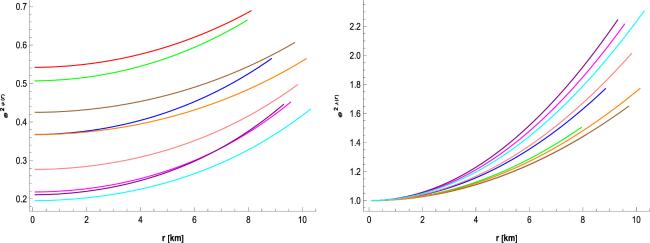
This subsection focuses on analyzing the behavior of the metric potentials defined in equations (28) and (29). By carefully selecting these potentials, we ensure that they remain continuous and free of singularities within the star. Moreover, we align them precisely with the external Bardeen models line element at the boundary. To investigate the properties of these potentials, we generated plots for the functions e2ψ and e2λ, as demonstrated in figure 1. The graphs indicate that e2ψ∣r=0 = β > 0 and e2λ∣r=0 = 1, confirming that both potentials are finite at the star's center and regular throughout the region r < rb. These profiles show a smooth and monotonically increasing trend with radial distance, a feature that is characteristic of a physically well-behaved stellar model.
Figure 1. Metric Potentials against radial coordinate r.
5.2. Energy density and pressure components
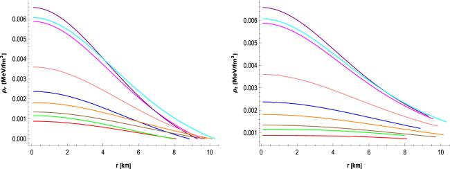
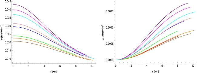
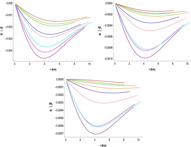
In this subsection, we explore the behaviors of ρ, pr, and pt, for different star models with varying masses and radii, as outlined in table 1. Given the complexity of their analytical forms, we rely on graphical representations to analyze these quantities. In figures 2 and 3 (left panel), we have plotted the radial pressure, tangential pressure, and energy density, respectively. The graphs reveal a consistent decreasing trend for ρ, pr, and pt, as a function of the radial coordinate r, with maximum values occurring at the star's core. Additionally, all three quantities remain non-negative within the star, and the radial pressure pr vanishes at the boundary r = rb, as expected. Moreover, gradients of energy density, radial pressure and tangential pressure can be seen in figure 4, which are zero at origin and become negative when we move towards the boundary of the star.
Figure 4. Graphical representation of gradients against r.
5.3. Anisotropy in pressure
This subsection will discuss very important characteristics of stellar structure, which is anisotropy. Given that we are considering an anisotropic matter distribution, where the radial and tangential pressure components pr and pt differ, it is essential to examine the behavior of the anisotropic factor, denoted by Δ = pt − pr. This factor provides valuable insights into how the pressures diverge within the star and plays a significant role in assessing the internal structure and stability. Analyzing Δ allows us to better understand the effects of anisotropy on the dynamics and physical properties of the stellar model. In view of equations (32) and (33), the equation for the anisotropy is given as
$\begin{eqnarray}\begin{array}{l}\alpha {{ \mathcal A }}^{11}\left(16L{r}^{2}X{Y}^{2}+1\right)-\alpha {r}^{2}{{ \mathcal A }}^{22}+\frac{\alpha }{r\left({r}^{2}Y+1\right)\left(16L{r}^{2}X{Y}^{2}+1\right)}\\ \,\times \,\left[r\left\{Y\left(-4{r}^{2}XY({{ \mathcal A }}_{0}^{0}{{ \mathcal A }}^{00})\left({r}^{2}Y+1\right)+32LXY\right.\right.\right.\\ \quad \times \,({{ \mathcal A }}_{1}^{1}{{ \mathcal A }}^{11})\left(2{r}^{2}Y+1\right)+r\left(2r({{ \mathcal A }}_{2}^{2}{{ \mathcal A }}^{22})-X({{ \mathcal A }}_{0}^{0}{{ \mathcal A }}^{00})^{\prime} {\left({r}^{2}Y+1\right)}^{2}\right.\\ \quad \left.\left.+\,2({{ \mathcal A }}_{1}^{1}{{ \mathcal A }}^{11})^{\prime} \left(8LXY\left(2{r}^{2}Y+1\right)+1\right)\right)\right)\\ \quad \left.\left.+\,2({{ \mathcal A }}_{2}^{2}{{ \mathcal A }}^{22})+r({{ \mathcal A }}_{2}^{2}{{ \mathcal A }}^{22})^{\prime} \left({r}^{2}Y+1\right)\right\}+({{ \mathcal A }}_{1}^{1}{{ \mathcal A }}^{11})^{\prime} \right]\\ \quad -\,\frac{1}{2{r}^{2}{\left({r}^{2}Y+1\right)}^{2}{\left(16L{r}^{2}X{Y}^{2}+1\right)}^{2}}\left[\alpha \left\{2({{ \mathcal A }}_{1}^{1}{{ \mathcal A }}^{11})\left({r}^{2}Y\right.\right.\right.\\ \quad \times \,\left({r}^{2}Y\left(16LXY\left({r}^{2}Y\left(16LXY\left(5{r}^{2}Y+2\right)+11\right)\right.\right.\right.\\ \quad \left.\left.\left.\left.+\,16LXY+6\right)+5\right)+48LXY+2\right)+1\right)+{r}^{2}\left({r}^{2}Y+1\right)\\ \quad \times \,\left(4({{ \mathcal A }}_{2}^{2}{{ \mathcal A }}^{22})\left(2{r}^{2}Y\left(4LXY\left(3{r}^{2}Y+1\right)+1\right)+1\right)\right.\\ \quad +\,r\left(-2XY\left({r}^{2}Y+1\right)\left(16L{r}^{2}X{Y}^{2}+1\right)\left({r}^{2}Y({{ \mathcal A }}_{0}^{0}{{ \mathcal A }}^{00})^{\prime} \right.\right.\\ \quad \left.+\,({{ \mathcal A }}_{0}^{0}{{ \mathcal A }}^{00})^{\prime} -24LY({{ \mathcal A }}_{1}^{1}{{ \mathcal A }}^{11})^{\prime} \right)+2({{ \mathcal A }}_{2}^{2}{{ \mathcal A }}^{22})^{\prime} \\ \,\times \,\left(4{r}^{2}Y\left(2LXY\left(7{r}^{2}Y+5\right)+1\right)+3\right)+r({{ \mathcal A }}_{2}^{2}{{ \mathcal A }}^{22})^{\prime\prime} \left({r}^{2}Y+1\right)\\ \quad \left.\left.\left.\left.\times \,\left(16L{r}^{2}X{Y}^{2}+1\right)\right)\right)\right\}\right]-\frac{1}{2}\alpha ({{ \mathcal A }}_{1}^{1}{{ \mathcal A }}^{11})^{\prime\prime} -\frac{{E}^{2}}{4\pi }\\ \quad -\,16L{r}^{2}X{Y}^{2}{{ \mathcal R }}^{11}+{r}^{2}{{ \mathcal R }}^{22}-{{ \mathcal R }}^{11}={\rm{\Delta }}.\end{array}\end{eqnarray}$
Figure 3 (right panel) shows the profiles for the anisotropy factor and we may perceive that the difference between pr and pt components are seen to be zero at r = 0. The anisotropic function remains positive at the star's interior boundary, indicating that the anisotropic force will be repulsive.
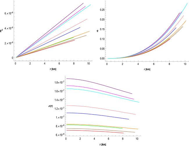
5.4. Electric field, charge and charge density
Figure 5 (left panel) shows the evolution of the electric field and it may be noticed from the figure that the electric field is more significant near the boundary and turns out to be zero at the center of all the stars under consideration and has a positive increasing nature in the domain 0 < r≤rb. Moreover, the graphical representation of charge and charge density can be seen in figure 5, which shows the variations from the center to the surface of the stars.
Figure 5. Graphical analysis of electric field, charge, and charge density against r.
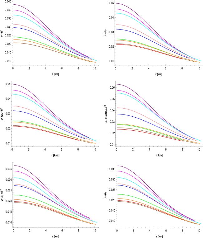
5.5. Energy conditions
Energy conditions are a very important aspect while discussing compact stars. The energy conditions include null energy conditions (NEC), weak energy conditions (WEC), strong energy conditions (SEC), and dominant energy conditions (DEC), which are defined as follows:
It can be noticed from figure 6 that all of these energy conditions are satisfied, which suggests that the proposed star models in the framework of Ricci-inverse gravity, are physically acceptable.
Figure 6. Graphical analysis of energy conditions against r.
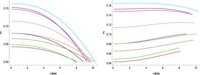
5.6. Equation of state parameters
The equation of state (EoS) defines a relation between pr and ρ, as well as pt and ρ. There are many types of EoS parameters in the literature, but we prefer radial EoS pressure ωr and tangential EoS pressure ωt, which are defined as follows
It is also a mandatory condition that both of these EoS parameters should lie between zero and one. It can be seen from figure 7 that the parameters ωr and ωt are both between 0 and 1 for every star under consideration in the domain 0≤r≤rb, which means that both parameters satisfy the given condition.
Figure 7. Graphical representation of EoS parameters against r.
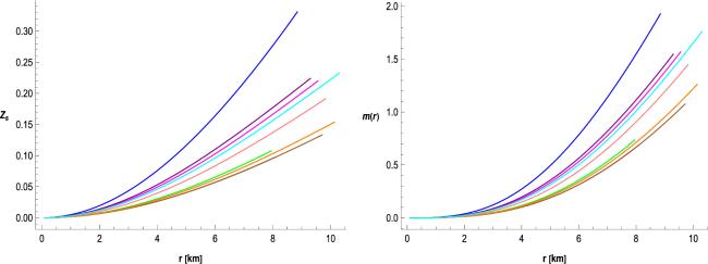
5.7. Mass function, compactness factor and surface redshift function
In this subsection, we will examine key functions of our model, such as the mass function m(r), the compactness factor u(r), and the surface redshift Zs. The mass function m(r) is defined as follows
The graphical behavior as seen in figure 8 (right panel) clearly shows that there is no singularity in the function m(r) and it exhibits consistently increasing behavior and has reached its maximum value at the surface of the star. Also, the graphical illustration shows that when r → 0, m(r) → 0, showing the regularity at the center of the stars. Moreover, the compactness factor is also defined as
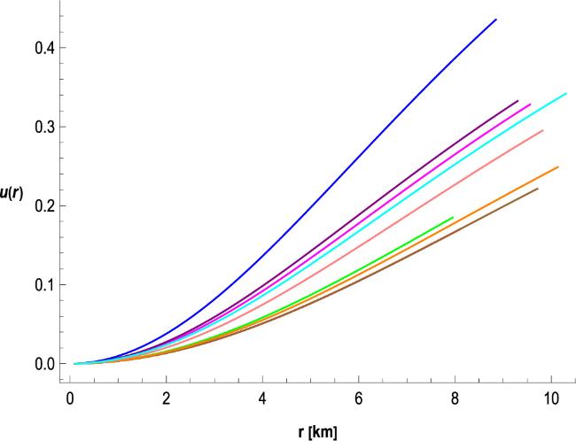
The compactness factor u(r) is critical for understanding the gravitational properties and stability of these dense objects. Buchdahl [104] showed that u(r) has an upper bound of 8/9, so that it does not proceed to a gravitational collapse. The graphical representation of u(r) is shown in figure 9, which demonstrates monotonically increasing behavior against r and we also observe that the Buchdahl limit is also not violated. Now, the surface redshift function Zs is expressed as
The graphical evolution of Zs can be seen in the left panel of figure 8, which shows the increasing behavior of Zs and its maximum value at the star's surface.
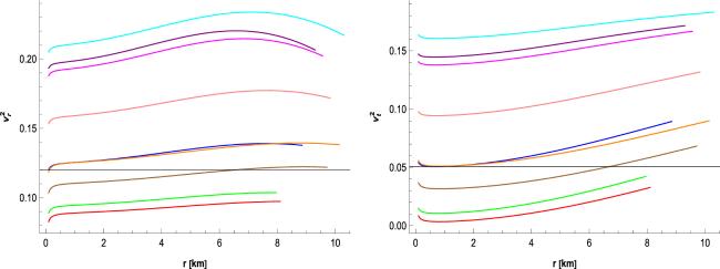
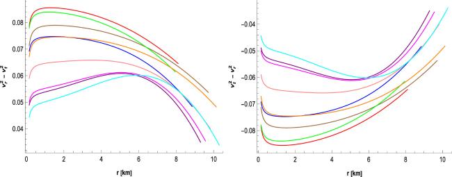
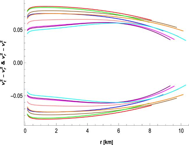
According to Herrera [105], these sound speeds must meet the causality condition for both the radial and transverse pressure components. This means that the speed of sound must satisfy the restrictions $0\leqslant {v}_{r}^{2}\leqslant 1$ and $0\leqslant {v}_{t}^{2}\leqslant 1$. It can be noticed from figure 10 that both of these components i.e., ${v}_{r}^{2}$ and ${v}_{t}^{2}$, must satisfy the given range [0, 1] at every point within the boundary of stellar objects. Abreu [106] introduced a concept for examining the stable and unstable configurations of celestial objects i.e., $| {v}_{t}^{2}-{v}_{r}^{2}| \leqslant 1$. It can be noticed from figures 11 and 12 that the differences of both sound speeds ${v}_{r}^{2}$ and ${v}_{t}^{2}$ satisfies the Abreu's condition, which means that our considered stars are stable.
Figure 12. Graphical representation of Abrea condition (combined behavior) against r.
5.9. Stability analysis via adiabatic index
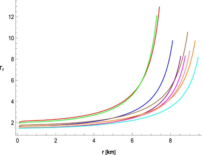
In this subsection, we look at a key ratio called the adiabatic index (Γr), to check the stability of the compact stars. Firstly, Chen et al [107] introduced the concept of the adiabatic index for an isotropic fluid sphere. Later on, Chandrasekhar [108] was one of the pioneers who used the adiabatic index to examine the stability region of a compact stars. The adiabatic index is defined as
According to Heintzmann and Hillebrandt [109], the stellar objects are considered to be stable when the value of Γr is greater than 4/3, otherwise it is unstable. It can be noticed from figure (13) that Γr is an increasing function of r and ${{\rm{\Gamma }}}_{r}\gt \frac{4}{3}$, which means that our considered compact stars are stable.
Figure 13. Graphical representation of adiabatic index against r.
5.10. Stability analysis via equilibrium condition
The Tolman–Oppenheimer–Volkoff (TOV) equation is crucial for studying the equilibrium conditions of compact objects. To evaluate the stability of our model, we derived a modified version of the TOV equation within the framework of $f({ \mathcal R },{ \mathcal A })$ gravity theory. This modification leads to the following equation, as derived from equation (8):
$\begin{eqnarray}\begin{array}{l}\frac{{\rm{d}}{p}_{r}}{{\rm{d}}r}+\left(\rho +{p}_{r}\right)\psi ^{\prime} -\frac{2{\rm{\Delta }}}{r}-\alpha \left\{-\left(\psi ^{\prime} +2\lambda ^{\prime} +\frac{2}{r}\right){{\rm{e}}}^{2\lambda }{{ \mathcal A }}^{11}\right.\\ \quad \left.-\,\psi ^{\prime} {{\rm{e}}}^{2\psi }{{ \mathcal A }}^{00}+2r{{ \mathcal A }}^{22}\Space{0ex}{2.75ex}{0ex}\right\}+\frac{\alpha }{2}({ \mathcal A })^{\prime} +\alpha {{\rm{e}}}^{2\lambda }({{ \mathcal A }}^{11})^{\prime} \\ \quad -\,\frac{\alpha }{2{r}^{3}}\left[\left(-10r+8{r}^{2}\lambda ^{\prime} +4{r}^{3}\lambda ^{\prime} \psi ^{\prime} -6{r}^{3}\psi {{\prime} }^{2}-{r}^{3}\psi ^{\prime\prime} \right)\right.\\ \,\times \,({{ \mathcal A }}_{1}^{1}{{ \mathcal A }}^{11})^{\prime} +\left(2{r}^{2}+2{r}^{3}\psi ^{\prime} \right)({{ \mathcal A }}_{1}^{1}{{ \mathcal A }}^{11})^{\prime\prime} +{{\rm{e}}}^{-2\lambda }\\ \quad \times \,\left(2{r}^{3}+4{r}^{4}\lambda ^{\prime} \right)({{ \mathcal A }}_{2}^{2}{{ \mathcal A }}^{22})^{\prime} -2{r}^{4}{{\rm{e}}}^{-2\lambda }({{ \mathcal A }}_{2}^{2}{{ \mathcal A }}^{22})^{\prime\prime} \\ \quad +\,{r}^{3}\psi ^{\prime} {{\rm{e}}}^{-2\lambda }({{ \mathcal A }}_{0}^{0}{{ \mathcal A }}^{00})^{\prime\prime} +\left(-2{r}^{3}\psi ^{\prime} \lambda ^{\prime} +{r}^{3}\psi ^{\prime\prime} \right)({{ \mathcal A }}_{0}^{0}{{ \mathcal A }}^{00})^{\prime} \\ \quad +\,\left(16+8{r}^{2}\lambda {{\prime} }^{2}+4{r}^{3}\psi ^{\prime} \lambda {{\prime} }^{2}+4{r}^{2}\lambda ^{\prime\prime} +4{r}^{3}\psi {{\prime} }^{3}+2{r}^{3}\psi ^{\prime} \lambda ^{\prime\prime} \right.\\ \quad \left.\left.-\,4{r}^{3}\psi ^{\prime} \psi ^{\prime\prime} -12r\lambda ^{\prime} -8{r}^{3}\lambda ^{\prime} \psi {{\prime} }^{2}-2{r}^{3}\lambda ^{\prime} \psi ^{\prime\prime} \right){{ \mathcal A }}_{1}^{1}{{ \mathcal A }}^{11}\right]\\ \quad -\,\sigma E{{\rm{e}}}^{\lambda }=0.\end{array}\end{eqnarray}$
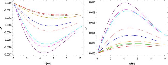
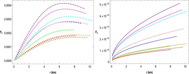
The above mentioned equation (54) establishes the configuration's equilibrium condition under the gravitational force (Fg), hydrostatic force (Fh), anisotropic force (Fa), and electric charge force (Fe). Now, one can rewrite equation (54) as
$\begin{eqnarray}\begin{array}{rcl}{F}_{{\rm{g}}} & = & \left(\rho +{p}_{r}\right)\psi ^{\prime} -\alpha \left[-\left(\psi ^{\prime} +2\lambda ^{\prime} +\frac{2}{r}\right){e}^{2\lambda }{{ \mathcal A }}^{11}-\psi ^{\prime} {e}^{2\psi }{{ \mathcal A }}^{00}\right.\\ & & \left.+2r{{ \mathcal A }}^{22}\right]+\frac{\alpha }{2}({ \mathcal A })^{\prime} +\alpha {e}^{2\lambda }({{ \mathcal A }}^{11})^{\prime} \\ & & -\frac{\alpha }{2{r}^{3}}\left[\left(-10r+8{r}^{2}\lambda ^{\prime} +4{r}^{3}\lambda ^{\prime} \psi ^{\prime} -6{r}^{3}\psi {{\prime} }^{2}-{r}^{3}\psi ^{\prime\prime} \right)\right.\\ & & \times ({{ \mathcal A }}_{1}^{1}{{ \mathcal A }}^{11})^{\prime} +\left(2{r}^{2}+2{r}^{3}\psi ^{\prime} \right)({{ \mathcal A }}_{1}^{1}{{ \mathcal A }}^{11})^{\prime\prime} \\ & & +{e}^{-2\lambda }\left(2{r}^{3}+4{r}^{4}\lambda ^{\prime} \right)({{ \mathcal A }}_{2}^{2}{{ \mathcal A }}^{22})^{\prime} -2{r}^{4}{e}^{-2\lambda }({{ \mathcal A }}_{2}^{2}{{ \mathcal A }}^{22})^{\prime\prime} \\ & & +{r}^{3}\psi ^{\prime} {e}^{-2\lambda }({{ \mathcal A }}_{0}^{0}{{ \mathcal A }}^{00})^{\prime\prime} +\left(-2{r}^{3}\psi ^{\prime} \lambda ^{\prime} +{r}^{3}\psi ^{\prime\prime} \right)({{ \mathcal A }}_{0}^{0}{{ \mathcal A }}^{00})^{\prime} \\ & & +\left(16+8{r}^{2}\lambda {{\prime} }^{2}+4{r}^{3}\psi ^{\prime} \lambda {{\prime} }^{2}+4{r}^{2}\lambda ^{\prime\prime} +4{r}^{3}\psi {{\prime} }^{3}+2{r}^{3}\psi ^{\prime} \lambda ^{\prime\prime} \right.\\ & & \left.\left.-4{r}^{3}\psi ^{\prime} \psi ^{\prime\prime} -12r\lambda ^{\prime} -8{r}^{3}\lambda ^{\prime} \psi {{\prime} }^{2}-2{r}^{3}\lambda ^{\prime} \psi ^{\prime\prime} \right){{ \mathcal A }}_{1}^{1}{{ \mathcal A }}^{11}\right].\end{array}\end{eqnarray}$
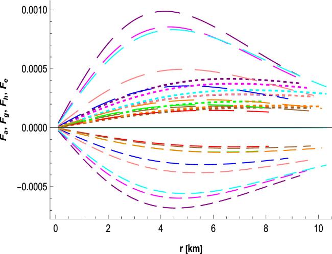
Note that when α = 0, which corresponds to the case of general relativity, the expression for the gravitational force Fg from equation (57) simplifies to ${F}_{{\rm{g}}}=(\rho +{p}_{r})\psi ^{\prime} $, a well-known result. The additional terms in the expression for Fg arise from the inclusion of ${ \mathcal A }$ in the function $f({ \mathcal R },{ \mathcal A })$ as specified in equation (3). The graphical representation of all these forces including Fh, Fa, Fe and Fg can be visualized in figures (14) and (15). The visual representations of the forces show that Fh, Fe, and Fa are positive (i.e. repulsive in nature), and these forces will counterbalance the Fg, which is negative (i.e. attractive in nature). The combined graphical representation of all these forces can be seen in figure (16), which ultimately leads to the formation of a stable, compact celestial object.
Figure 16. Graphical representation of all forces against r.
6. Concluding remarks
Modified theories of gravity play a significant role in investigating the cosmos dynamics and has become important, even if GR has been highly successful. The challenge of determining an appropriate model to depict the intricate geometry of compact objects has garnered attention in the extended theories of gravity. In this study, we looked at the charged anisotropic stellar model using the modified Ricci-inverse gravity framework, which is an extension of GR. This modified Ricci-inverse theory has been recently introduced in 2020. Modeling the astrophysical objects poses significant challenges using $f({ \mathcal R },{ \mathcal A })$. Due to the complexities of this modified gravity's field equation, we opted for the linear model: $f({ \mathcal R },{ \mathcal A })={ \mathcal R }+\alpha { \mathcal A }$. We have formulated the stellar model using the Finch–Skea metric potentials, which comprise the arbitrary constants L, X, and Y. Our analysis has accounted for various compact stars whose masses and radii are provided in table 1. Through the utilization of the observed masses and radii of these stars, we have computed the values of the aforementioned arbitrary constants by aligning the inner spacetime with Bardeen spacetime. The compatibility of the calculated solutions with the physically acceptable range of the model is underscored by several key aspects demonstrated in this study. Firstly, the analysis reveals that the metric potentials, energy density, and pressure components maintain positivity and regularity throughout the stellar interior, indicating a stable configuration that aligns with physical expectations. Additionally, the solutions satisfy crucial energy conditions, such as the weak, strong, and dominant energy conditions, which are essential for any physically viable model. The results also show that the radial pressure diminishes to zero at the boundary of the star, further reinforcing the model's consistency with known physical behaviors in astrophysical objects. Furthermore, the analysis of the sound speed reveals that it remains within the permissible limits, satisfying causality requirements throughout the stellar distribution. These considerations collectively affirm that the solutions derived in this study reside within the physically acceptable range, thereby contributing to the overall viability and robustness of the proposed models in the context of anisotropic stellar configurations. The physical analysis of our results reveals that this anisotropic stellar model in $f({ \mathcal R },{ \mathcal A })$ gravity exhibits the following conclusive properties:
The metric potentials e2ψ and e2λ are positive and regular throughout the entire stellar interior, without any singularities as depicted in figure 1. This regularity underscores the reliability of the metric potentials in characterizing the gravitational dynamics within the star.
The graphical representation of energy density ρ and pressure components (pr, pt) are positive and monotonically decreasing across the inner domain of the stars as shown in figures 2 and 3. It can also be noticed that the radial pressure vanishes at the boundary r = rb and is highest at the core of the star.
The stellar models in Ricci-inverse gravity satisfy the following inequalities
The right panel of figure 3 represents the behavior of Δ, which indicates that the anisotropic force is repulsive.
All the energy conditions in the presence of charge are satisfied as shown in figure 6.
The mass function and compactness factor, surface redshift function are positive and increasing in nature as plotted in figures 8 and 9.
The causality condition is satisfied as both radial and transverse sound speeds, i.e., lies between [0, 1], which indicates its physical consistency and potential stability throughout the stellar distribution in $f({ \mathcal R },{ \mathcal A })$ gravity.
The explicit graphs of all the forces are shown in figures 14 and 15. The positive nature of Fh, Fa, and Fe indicates that these forces are repulsive in nature, while the negative behavior of Fg suggests that the gravitational force is attractive. The combined graphical analysis of all the forces can be seen in figure 16, which demonstrates that our system is in a state of equilibrium.
In this work, we have investigated the physical behavior of compact stars in the framework of Ricci-inverse gravity. As a result of all the notable findings, it is evident that we can build a viable, stable, and singularity-free generalized stellar model within the interior anisotropic fluid distribution. Hence, it is possible to analyze the physical characteristics of compact star entities using theoretical and astrophysical methods through the study of an exceptionally dense and celestial bodies. All the analysis leads to the conclusion that the compact stars model presented in this work adequately clarifies the physical requirements in the framework of Ricci-inverse gravity.
For future work, our solutions can serve as a foundation for exploring the complexity-free anisotropic Finch–Skea model that satisfies the Karmarkar condition, allowing for a more nuanced understanding of charged anisotropic structures. Additionally, the insights gained from our study may illuminate the structure of anisotropic fuzzy dark matter, providing a framework for investigating its implications on cosmological scales. Moreover, we acknowledge the importance of studying the imprints of dark matter on the structural properties of minimally deformed compact stars, which can be a significant topic for further investigation. This could lead to a deeper understanding of how dark matter influences stellar dynamics and stability. Lastly, our findings can be instrumental in constructing charged cylindrical gravastar-like structures, which represent an intriguing class of compact objects in modified gravity theories. By applying our models to these structures, researchers may gain valuable insights into their stability, gravitational behavior, and potential observational signatures. We will ensure to integrate these applications into the conclusion of our paper, thereby emphasizing the broader implications and future research directions arising from our work. Thank you for highlighting these critical points, which will enhance the overall impact and clarity of our study.
Appendix
$\begin{eqnarray*}{{ \mathcal R }}^{00}=\frac{64L{r}^{2}X{Y}^{3}+6Y}{X{\left({r}^{2}Y+1\right)}^{3}{\left(16L{r}^{2}X{Y}^{2}+1\right)}^{2}},\end{eqnarray*}$
$\begin{eqnarray*}{{ \mathcal R }}^{11}=\frac{2Y\left(16LXY\left({r}^{2}Y+1\right)-1\right)}{\left({r}^{2}Y+1\right){\left(16L{r}^{2}X{Y}^{2}+1\right)}^{3}},\end{eqnarray*}$
$\begin{eqnarray*}{{ \mathcal R }}^{22}=\frac{2Y\left(16LXY\left(8L{r}^{2}X{Y}^{2}\left({r}^{2}Y+1\right)+1\right)-1\right)}{\left({r}^{2}Y+1\right){\left(16L{r}^{3}X{Y}^{2}+r\right)}^{2}},\end{eqnarray*}$
$\begin{eqnarray*}{ \mathcal R }=\frac{4Y\left(8LXY\left({r}^{2}Y\left(16LXY\left({r}^{2}Y+1\right)-1\right)+3\right)-3\right)}{\left({r}^{2}Y+1\right){\left(16L{r}^{2}X{Y}^{2}+1\right)}^{2}},\end{eqnarray*}$
$\begin{eqnarray*}{{ \mathcal A }}^{00}=\frac{{\left(16L{r}^{2}X{Y}^{2}+1\right)}^{2}}{2XY\left({r}^{2}Y+1\right)\left(32L{r}^{2}X{Y}^{2}+3\right)},\end{eqnarray*}$
$\begin{eqnarray*}{{ \mathcal A }}^{11}=\frac{\left({r}^{2}Y+1\right)\left(16L{r}^{2}X{Y}^{2}+1\right)}{2Y\left(16LXY\left({r}^{2}Y+1\right)-1\right)},\end{eqnarray*}$
$\begin{eqnarray*}{{ \mathcal A }}^{22}=\frac{\left({r}^{2}Y+1\right){\left(16L{r}^{2}X{Y}^{2}+1\right)}^{2}}{2{r}^{2}Y\left(16LXY\left(8L{r}^{2}X{Y}^{2}\left({r}^{2}Y+1\right)+1\right)-1\right)},\end{eqnarray*}$
$\begin{eqnarray*}({{ \mathcal A }}^{11})^{\prime} =\frac{2r(8LXY-1)}{{\left(1-16LXY\left({r}^{2}Y+1\right)\right)}^{2}}+r,\end{eqnarray*}$
$\begin{eqnarray*}{ \mathcal A }=\frac{\left({r}^{2}Y+1\right){\left(16L{r}^{2}X{Y}^{2}+1\right)}^{2}}{2Y\left(16LXY\left({r}^{2}Y+1\right)-1\right)}+\frac{\left({r}^{2}Y+1\right){\left(16L{r}^{2}X{Y}^{2}+1\right)}^{2}}{Y\left(16LXY\left(8L{r}^{2}X{Y}^{2}\left({r}^{2}Y+1\right)+1\right)-1\right)}-\frac{\left({r}^{2}Y+1\right){\left(16L{r}^{2}X{Y}^{2}+1\right)}^{2}}{64L{r}^{2}X{Y}^{3}+6Y},\end{eqnarray*}$
$\begin{eqnarray*}{{ \mathcal A }}_{0}^{0}{{ \mathcal A }}^{00}=-\frac{{\left(16L{r}^{2}X{Y}^{2}+1\right)}^{4}}{2XY\left(32L{r}^{2}X{Y}^{2}+3\right)\left(64L{r}^{2}X{Y}^{3}+6Y\right)},\end{eqnarray*}$
$\begin{eqnarray*}{{ \mathcal A }}_{1}^{1}{{ \mathcal A }}^{11}=\frac{{\left({r}^{2}Y+1\right)}^{2}{\left(16L{r}^{2}X{Y}^{2}+1\right)}^{3}}{4{Y}^{2}{\left(16LXY\left({r}^{2}Y+1\right)-1\right)}^{2}},\end{eqnarray*}$
$\begin{eqnarray*}{{ \mathcal A }}_{2}^{2}{{ \mathcal A }}^{22}=\frac{{\left({r}^{2}Y+1\right)}^{2}{\left(16L{r}^{2}X{Y}^{2}+1\right)}^{4}}{4{r}^{2}{Y}^{2}{\left(16LXY\left(8L{r}^{2}X{Y}^{2}\left({r}^{2}Y+1\right)+1\right)-1\right)}^{2}},\end{eqnarray*}$
$\begin{eqnarray*}({{ \mathcal A }}_{0}^{0}{{ \mathcal A }}^{00})^{\prime} =-\frac{64Lr\left(8L{r}^{2}X{Y}^{2}+1\right){\left(16L{r}^{2}X{Y}^{2}+1\right)}^{3}}{{\left(32L{r}^{2}X{Y}^{2}+3\right)}^{3}},\end{eqnarray*}$
$\begin{eqnarray*}({{ \mathcal A }}_{1}^{1}{{ \mathcal A }}^{11})^{\prime} =\frac{r\left({r}^{2}Y+1\right){\left(16L{r}^{2}X{Y}^{2}+1\right)}^{2}\left(8LXY\left({r}^{2}Y\left(48LXY\left({r}^{2}Y+2\right)-5\right)+48LXY-3\right)-1\right)}{Y{\left(16LXY\left({r}^{2}Y+1\right)-1\right)}^{3}},\end{eqnarray*}$
$\begin{eqnarray}\begin{array}{l}({{ \mathcal A }}_{2}^{2}{{ \mathcal A }}^{22})^{\prime} =\frac{1}{2{r}^{3}{Y}^{2}{\left(16LXY\left(8L{r}^{2}X{Y}^{2}\left({r}^{2}Y+1\right)+1\right)-1\right)}^{3}}\\ \,\times \,\left[\left({r}^{2}Y+1\right){\left(16L{r}^{2}X{Y}^{2}+1\right)}^{3}\left\{{r}^{2}Y\left(16LXY\right.\right.\right.\\ \,\times \,\left({r}^{2}Y\left(8LXY\left({r}^{2}Y\left(16LXY\left({r}^{2}Y+2\right)-3\right)+16LXY\right.\right.\right.\\ \quad \left.\left.\left.\left.\left.\left.+\,4\right)-5\right)+24LXY-2\right)-1\right)-16LXY+1\right\}\right],\end{array}\end{eqnarray}$
$\begin{eqnarray*}({{ \mathcal A }}_{0}^{0}{{ \mathcal A }}^{00})^{\prime\prime} =-\frac{64L{\left(16L{r}^{2}X{Y}^{2}+1\right)}^{2}\left(8L{r}^{2}X{Y}^{2}\left(16L{r}^{2}X{Y}^{2}\left(96L{r}^{2}X{Y}^{2}+25\right)+31\right)+3\right)}{{\left(32L{r}^{2}X{Y}^{2}+3\right)}^{4}},\end{eqnarray*}$
The authors extend their appreciation to the Deanship of Research and Graduate Studies at King Khalid University for funding this work through Large Research Project under Grant No. RGP2/30/45.
WangD et al 2023 Observational constraints on a logarithmic scalar field dark energy model and black hole mass evolution in the Universe Eur. Phys. J. C83 1 14
MalikA2024 Charged stellar structure with Krori–Barua potentials in f(R, φ, X) gravity admitting Chaplygin equation of state Int. J. Geom. Meth. Mod. Phys.21 2450157
AsgharZ et al 2023 Comprehensive analysis of relativistic embedded class-I exponential compact spheres in f(R, φ) gravity via Karmarkar condition Comm. Theor. Phys.75 105401
YouL et al 2023 Finite-time stabilization for uncertain nonlinear systems with impulsive disturbance via aperiodic intermittent control Appl. Math. Comput.443 127782
MalikA et al 2024 Stability analysis of anisotropic stellar structures in Rastall theory of gravity utilizing cracking technique Chin. J. Phys.89 613 627
YuM et al 2023 Exponential stabilization of nonlinear systems under saturated control involving impulse correction Nonlinear Anal. Hybrid Syst.48 101335
WuJ et al 2022 Finite-time stabilization of time-varying nonlinear systems based on a novel differential inequality approach Appl. Math. Comput.420 126895
MalikA et al 2024 Investigation of charged stellar structures in f(R, φ) gravity using Reissner–Nordstrom geometry Int. J. Geom. Meth. Mod. Phys.21 2450099
ChenW et al 2022 Positive ground states for nonlinear Schrdinger–Kirchhoff equations with periodic potential or potential well in R3Bound. Value Probl.97


