


1. Introduction
The Rayleigh–Taylor instability (RTI) can occur at the interface between two fluids of different densities or fluids with sharp density gradients when a heavier fluid is accelerated by a lighter one under the influence of the gravitational force and the magnetic field [1–5]. In classical plasmas, the RTI growth rate gets enhanced due to the density difference of fluids by $\tilde{\gamma }=\sqrt{{A}_{T}kg}$, where AT, k, and g are, respectively, the Atwood number, perturbed wavenumber, and gravitational force. The RTI can also occur in inertial confinement fusion (ICF) [6] and several astrophysical environments, such as Crab Nebula [7], interacting supernova [8], supernova remnants [9], white dwarfs [10, 11], neutron star [12, 13], and disk magnetosphere interface [14] where the rare magnetospheric plasma provides a support to highly dense matter against the gravitational force. Chandrasekhar [4] first investigated the linear dispersive properties of waves propagating at the interface between two semi-infinite fluids in a Tokamak plasma. Later, it was advanced to study the instability analysis of an electrolyte solution in the presence of a strong magnetic field [15]. The theoretical developments on RTI are also noted in other plasma environments, e.g., dusty plasmas [16, 17], ionospheric region [18], dayside magnetopause [19, 20], etc. Here, the fluid viscosity and shear flow effects significantly affect the instabilities in a uniform magnetized plasma [21, 22].
Typically, astrophysical plasmas are highly dense and degenerate gas, and can also be strongly magnetized. In white dwarfs, the particle number density can vary in the range ni ≃ 1028 − 1030cm−3, the temperature varies from 106 K to 108 K, and the magnetic field ~ 104 − 108 G. So, the physical parameters, including the particle density, magnetic field, and the particle's temperature can play a significant role in the linear and nonlinear propagation of waves and instabilities in such plasma environments. The degenerate electrons may be non-relativistic, relativistic, or ultra-relativistic according to when the Fermi energy is much larger than, close to, or much smaller than the electron rest mass energy. Thus, it is pertinent to define a pressure law and the particle distribution that can efficiently describe the relevant physics of relativistic degenerate electron-ion (e-i) magnetoplasmas. In this context, several authors have studied linear and nonlinear properties of waves and instabilities in relativistic and non-relativistic plasmas [1, 23–29].
In recent work, Maryam et al [1] investigated the RTI in radiative dense electron-ion (e-i) plasmas, and they showed the wave phase velocity and the instability growth rate are influenced by the radiative pressure of electrons. Starting from a quantum hydrodynamic model, Bychkov et al [30] investigated the quantum effects on the internal waves and RTI in quantum plasmas. They showed that quantum pressure always stabilizes the RTI, and a specific form of pure quantum internal wave exists in the transverse direction. This type of internal wave was absent in classical plasmas and not influenced by the gravity force. The presence of an external magnetic field beside the quantum effect stabilized the RTI more, as studied by Hoshoudy [31]. Ali et al [32] studied the RTI in compressible quantum e-i magnetoplasmas with cold classical ions and inertialess electrons, and they showed that the quantum speed and density gradient scale length enhanced the growth rate of instability due to quantum correction associated with the Fermi pressure law and quantum Bohm potential force. In a similar study, Adak et al [33] reported the RTI in a pair-ion (positive and negative ions with equal masses but different temperatures) inhomogeneous plasma under the influences of the gravity force and the density gradient. They showed that the formation of RTI neither depends on the ion masses nor the growth rate of instability. A development in RTI has also been noted in a strongly coupled e-i quantum plasma under the influence of the shear viscosity, and the growth rate destabilizes irrespective of the direction of the gradient of shear viscosity [3]. Later, Bhambhu and Prajapati [23] studied the effects of compressibility, ultra-relativistic degenerate electrons, and strong coupling effect of classical ions on the density gradient-driven RTI opposite to the direction of gravity in unmagnetized plasmas. They showed that the Coulomb coupling parameter and isothermal compressibility of ion fluid significantly modify the growth rate of RTI in plasmas relevant to white dwarfs. In contrast, the ultra-relativistic degenerate pressure of electrons became insignificant in growth rate but significantly modified the existing regime of RTI; however, they did not consider the relativistic monition of electrons and ions and the finite temperature degeneracy of electrons. After that, authors studied the dispersion properties of RTI analytically in kinetic and hydrodynamic regimes with the effects of radiation pressure of ultra-relativistic degenerate electrons and strong magnetic field [2]. The viscosity and resistivity effects in low magnetized and high energy density e-i solar plasmas have been investigated numerically for high Atwood numbers on the formation of RTI [34]. The growth rate drastically changes due to adding the viscosity and resistivity effects as well as its internal structure to a small-scale limit. The magnetic field is explicitly independent of viscosity, and enstrophy and kinetic energy are independent of resistivity. More advancements in RTI and internal waves in strongly coupled in compressible quantum rotating plasmas can also be found [35]. Thus, in the current situation, RTI is an exciting problem for the researcher due to its several applications in laboratory plasmas and astrophysical environments.
From the above investigations, none of the authors have considered the effect of relativistic plasma fluid motion, fully degenerate, and partially degenerate pressures of electrons for advancing the existing theory of RTI in strongly magnetized e-i plasmas. Such advancement of RTI with analytical and numerical analyses will help better understand the observed phenomena in many degenerate astrophysical objects and laboratory plasmas. In this work, we study the possibility of the onset of RTI in a compressible inhomogeneous relativistic electron-ion magnetoplasma fluids under the influences of a strong uniform magnetic field, density gradient, and gravity force in three different cases when (i) electrons are classical or nondegenerate, (ii) electrons are fully degenerate, i.e., form a zero-temperature Fermi gas, and (iii) electrons are partially degenerate with Fermi energy higher than the electron thermal energy. Considering a two-fluid relativistic model for electrons and ions, we derive a general dispersion relation and analyze it for the RTI in the above three cases. The results show that the instability growth rate significantly differs as one switches from classical nondegenerate to degenerate regimes. We organize the manuscript in the following fashion, where we describe the physical model and the basic equations for the electron and ion fluids in section 2 . Section 3 demonstrates the linear theory of RTI and analyses the instability growth rates in three different regimes of classical, fully degenerate, and partially degenerate electrons. Finally, section 4 is left to summarize and conclude the main results.
2. The model and basic equations
We consider an inhomogeneous magnetized collisionless two-component electron-ion (e-i) plasma with a relativistic flow of electrons, which may be in isothermal equilibrium (nondegenerate or classical), fully degenerate (at zero temperature), or partially degenerate at finite temperature, and nondegenerate relativistic classical thermal ions. As shown in figure 1, we consider a plasma boundary in the yz-plane immersed in an external static uniform magnetic field, ${{\boldsymbol{B}}}_{0}={B}_{0}\hat{z}$ (In low-β plasmas, the magnetic field may be considered to be uniform) under the action of the constant gravitational field, ${\boldsymbol{g}}=g\hat{x}$ acting vertically downward. We assume that the background number density gradients for electrons and ions are along the negative x-axis, the wave propagation vector is k = (kx, ky, kz), and the electric field is E = (0, Ey, 0). At equilibrium, the uniform magnetic field acts as a light fluid to support the heavy two-component e-i plasmas and the Lorentz force balances the combined influence of the gravitational field force and the pressure gradient force. As a result, electrons and ions will drift (gravitational and diamagnetic drifts) in the opposite y-direction. If a perturbation in the interface develops due to random pressure fluctuations, these drift velocities of electrons and ions will cause charge separation and hence the generation of the perturbed electric field E (which changes sign as one goes from crest to trough in the perturbation). The latter will then produce E × B0-drift velocities for electrons and ions [in the upward (downward) direction where the plasma layer has moved upward (downward)]. The perturbation tends to grow at the expense of the potential energy of plasma (heavier) fluids in the gravitational field, which opposes the density gradient, and when the E × B0-drift velocities are properly phased. This leads to spikes in the heavier fluid penetrating lighter ones and the interface becomes unstable to form the RTI [36].
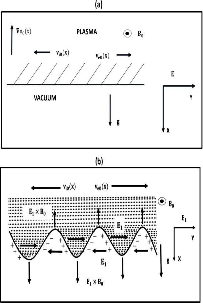
Figure 1. A schematic diagram for RTI showing the equilibrium state [Subplot (a)] and the perturbed state [Subplot (b)] of an electron-ion plasma under the influences of the gravity force, the electromagnetic fields, and the density gradient. |
As a starting point and to describe the dynamics of relativistic compressible electron and ion fluids in quasineutral plasmas, we consider the following dimensionless continuity and the momentum balance equations [24, 37].
$\begin{eqnarray}\frac{\partial \left({\gamma }_{j}{n}_{j}\right)}{\partial t}+{\boldsymbol{\nabla }}\cdot ({\gamma }_{j}{n}_{j}{{\boldsymbol{v}}}_{j})=0,\end{eqnarray}$
$\begin{eqnarray}\frac{{\rm{d}}}{{\rm{d}}{t}}\left(\frac{{H}_{j}{\gamma }_{j}{{\boldsymbol{v}}}_{j}}{{n}_{j}}\right)+\frac{{\rm{\nabla }}{P}_{j}}{{\gamma }_{j}{n}_{j}}=\frac{{m}_{i}{q}_{j}}{{m}_{j}e}\left({\boldsymbol{E}}+{{\rm{\Omega }}}_{i}{{\boldsymbol{v}}}_{j}\times \hat{z}\right)+\tilde{{\boldsymbol{g}}},\end{eqnarray}$
where ${\rm{d}}/{\rm{d}}{t}\equiv \partial /\partial t+\left({{\boldsymbol{v}}}_{j}\cdot {\rm{\nabla }}\right)$ is the total derivative, and the quantities nj, vj, and Pj are, respectively, the number density, velocity, and pressure of j-th species particles [j = i(e) for ions (electrons)], normalized by the unperturbed value nj0(0), the speed of light in vacuum c, and mjc2nj0(0) with mj denoting the mass of j-th species particles. Also, the electric field E is normalized by $\left({m}_{i}{c}^{2}/e{\lambda }_{s}\right)$, ${{\rm{\Omega }}}_{i}\left(={\omega }_{ci}/{\omega }_{pi}\right)$ is the ratio between the ion-cyclotron (ωci = eB0/mic) and ion plasma oscillation [${\omega }_{pi}={\left(4\pi {n}_{i0}(0){e}^{2}/{m}_{i}\right)}^{1/2}$] frequencies, Ωe = mΩi is the normalized electron-cyclotron frequency, m = mi/me is the ion to electron mass ratio, and $\tilde{{\boldsymbol{g}}}\,\left(={\boldsymbol{g}}/c{\omega }_{pi}\right)$ is the dimensionless gravity force per unit mass of the fluid. Furthermore, qj = e( − e) is the charge for positive ions (electrons), ${H}_{j}={{ \mathcal E }}_{j}+{P}_{j}$ is the enthalpy per unit volume of each fluid species j measured in the rest frame normalized by mjc2nj0(0) with ${{ \mathcal E }}_{j}$ denoting the total energy density, ${\gamma }_{j}\,\left(=1/\sqrt{1-{v}_{j}^{2}}\right)$ is the Lorentz factor for the j-th species particle, and the time t and the space x variables are normalized by the ion plasma period ${\omega }_{pi}^{-1}$ and the ion plasma skin depth λs( = c/ωpi) respectively.Due to their heavy inertia (compared to electrons), relativistic ions are treated as classical and nondegenerate. However, depending on the plasma environments (from laboratory low-density plasmas to astrophysical degenerate dense plasmas) electrons can deviate from the thermodynamic equilibrium and obey the Fermi–Dirac statistics. In the interior of stellar compact objects such as those of neutron stars and white dwarfs, not only do electrons have a relativistic speed, but also have an arbitrary degree of degeneracy, i.e., they are either partially degenerate at finite temperature or fully degenerate at zero temperature. Thus, their pressure equations vary. In section 3 , we will discuss the RTI in three different cases separately, using three different equations of state for electrons, and show how the instability growth rates differ in different plasma environments.
In what follows, we consider the variations of the unperturbed number density and the pressure along the x-axis. For adiabatic thermal ions, we write the equation of state as
$\begin{eqnarray}\frac{{P}_{i}}{{P}_{i0}(x)}={\left(\frac{{n}_{i}}{{n}_{i0}(x)}\right)}^{{\rm{\Gamma }}},\end{eqnarray}$
where ${P}_{i0}(x)\,\left(={\beta }_{i}{n}_{i0}(x)\right)$ is the unperturbed ion pressure normalized by ni0(0)mic2 and βi,e = kBTi,e/mi,ec2 is the relativity parameter for thermal ions (electrons). We also denote σ = Ti/Te as the ion to electron temperature ratio. Note that while βi is a parameter for the cases of both classical and degenerate (partially and fully) plasmas, the parameter βe appears only in classical and partially degenerate plasmas. The normalized enthalpy for the ion species is Hi = PiΓ/(Γ − 1) + ni, where the polytropic index Γ varies in 4/3 ≤ Γ ≤ 5/3. In the classical limit of ion thermal motions, Γ = 5/3 and Pi ≪ ni, while in the ultra-relativistic limit, we have Γ = 4/3 and Pi ≫ ni. Next, we assume the unperturbed plasma number densities and the pressure inhomogeneities to vary as $\begin{eqnarray}{n}_{j0}(x),\,{P}_{j0}(x)\unicode{x0007E}\exp \left(-x/{L}_{n}\right),\end{eqnarray}$
where Ln is the length scale of inhomogeneity normalized by λs.3. Rayleigh–Taylor instability
In this section, we study the RTI of electrostatic plane wave perturbations in relativistic e-i magnetoplasmas by deriving a general linear dispersion relation in the low-frequency limit: ${(\omega -{k}_{y}{v}_{j0}(x))}^{2}\ll {{\rm{\Omega }}}_{j}^{2};\,(j=i,e)$, where ω(ky) is the wave frequency (wave number) of perturbations and vj0(x) is the drift velocity of the j-th species particle along the y-axis. However, before deriving the dispersion relation for the perturbation, it is pertinent to consider the equilibrium plasma state.
At equilibrium, the momentum equation for the j-th species particles gives 6 )–(7 ), it is clear that the ions and electrons drift in opposite directions along the y-axis with velocities vi0(x) and ve0(x) due to the gravitational and diamagnetic drifts. Note that at equilibrium, there is no DC electric field. So, the E × B0-drift velocity is zero.
$\begin{eqnarray}\begin{array}{l}\left({{\boldsymbol{v}}}_{j0}(x)\cdot {\rm{\nabla }}\right)\left(\frac{{H}_{j0}(x){\gamma }_{j0}(x){{\boldsymbol{v}}}_{j0}(x)}{{n}_{j0}(x)}\right)\\ +\frac{{\rm{\nabla }}{P}_{j0}(x)}{{\gamma }_{j0}(x){n}_{j0}(x)}=\frac{{m}_{i}{q}_{j}}{{m}_{j}e}{{\rm{\Omega }}}_{i}\left({{\boldsymbol{v}}}_{j0}(x)\times \hat{z}\right)+\tilde{{\boldsymbol{g}}},\end{array}\end{eqnarray}$
from which we obtain the drift velocities for ions and electrons as [36] $\begin{eqnarray}{{\boldsymbol{v}}}_{i0}(x)\approx -\frac{1}{{{\rm{\Omega }}}_{i}}\left[\tilde{g}+\frac{{\beta }_{i}}{{\gamma }_{i0}(0){L}_{n}}\right]\hat{y},\end{eqnarray}$
$\begin{eqnarray}{{\boldsymbol{v}}}_{e0}(x)\approx \frac{1}{{{\rm{\Omega }}}_{e}}\left[\tilde{g}+\frac{{P}_{e0}(0)}{{\gamma }_{i0}(0){L}_{n}}\right]\hat{y},\end{eqnarray}$
where He0(x) = αene0(x) and Hi0(x)/ni0(x) = 1 + βiΓ/(Γ − 1). Also, ${\gamma }_{j0}(x)\approx {\gamma }_{j0}(0)={\left[1-{v}_{j0}^{2}(0)\right]}^{-1/2}$ and ${L}_{n}^{-1}\,=-\left(1/{n}_{j0}(x)\right)\left(\partial {n}_{j0}(x)/\partial x\right)=-\left(1/{P}_{j0}(x)\right)\left(\partial {P}_{j0}(x)/\partial x\right)$. From equations (To obtain the dispersion relation for electrostatic perturbations, we split up the dependent variables into their equilibrium and perturbation parts, i.e. nj = nj0(x) + nj1, vj = vj0(x) + vj1, E = 0 + E1, Pe = Pe0(x) + Pe1, etc. Assuming the perturbations to vary as plane waves of the form $\unicode{x0007E}\exp ({\rm{i}}{\boldsymbol{k}}\cdot {\boldsymbol{r}}-{\rm{i}}\omega t)$, where the wave vector k and the wave frequency ω are normalized by ${\lambda }_{s}^{-1}$ and ωpi respectively, we obtain from equation (2 ), the following reduced equation.8 ), the perpendicular components of the ion velocity are obtained as [1]
$\begin{eqnarray}\begin{array}{l}-{\rm{i}}\left(\omega -{k}_{y}{v}_{i0}(x)\right)\left[\frac{{\gamma }_{i0}(x){{\boldsymbol{v}}}_{i0}(x){n}_{i1}}{{n}_{i0}(x)}\left(\frac{{H}_{i1}}{{n}_{i1}}-\frac{{H}_{i0}(x)}{{n}_{i0}(x)}\right)\right.\\ +\left.\frac{{H}_{i0}(x)}{{n}_{i0}(x)}\left({\gamma }_{i1}{{\boldsymbol{v}}}_{i0}(x)+{\gamma }_{i0}(x){{\boldsymbol{v}}}_{i1}\right)\right]={{\boldsymbol{E}}}_{1}+{{\rm{\Omega }}}_{i}\left({{\boldsymbol{v}}}_{i1}\times \hat{z}\right),\end{array}\end{eqnarray}$
where Hi1/ni1 = 1 + βiΓ2/(Γ − 1). From equation ( $\begin{eqnarray}{v}_{i1x}=\frac{{E}_{1y}}{{{\rm{\Omega }}}_{i}},\end{eqnarray}$
$\begin{eqnarray}{v}_{i1y}=-{\rm{i}}{\alpha }_{i}\frac{\left(\omega -{k}_{y}{v}_{i0}(x)\right)}{{{\rm{\Omega }}}_{i}}\frac{{E}_{1y}}{{{\rm{\Omega }}}_{i}},\end{eqnarray}$
where αi ≈ γi0(0)Hi0(x)/ni0(x) and γi1 = vi0(x)vi1y.Next, from equation (1 ), the linearized ion continuity equation gives
$\begin{eqnarray}\begin{array}{l}\left[\omega -{k}_{y}{v}_{i0}(x)\right]\left[{\gamma }_{i0}(0){n}_{i1}+{\gamma }_{i1}{n}_{i0}(x)\right]\\ \quad -{\gamma }_{i0}(0){k}_{y}{n}_{i0}(x){v}_{i1y}\\ -{\gamma }_{i0}(0){n}_{i0}(x)\left({k}_{x}+\frac{{\rm{i}}}{{L}_{n}}\right){v}_{i1x}=0.\end{array}\end{eqnarray}$
Substituting equations (9 ) and (10 ) into equation (11 ), we obtain 2 ) the following expressions for the electron velocity (perturbed) components.13 )–(15 ) into the linearized electron continuity equation [to be obtained from equation (1 ) for electrons, i.e., for j = e], we obtain
$\begin{eqnarray}\frac{{E}_{1y}}{{{\rm{\Omega }}}_{i}}=\frac{{\rm{i}}{n}_{i1}}{{n}_{i0}(x)}\left(\frac{\omega -{k}_{y}{v}_{i0}(x)}{{\alpha }_{i}{k}_{y}\left(\omega -{k}_{y}{v}_{i0}(x)\right)/{{\rm{\Omega }}}_{i}-1/{L}_{n}+{\rm{i}}{k}_{x}}\right).\end{eqnarray}$
This expression for the electric field perturbation agrees with [1] after one has fixed the normalization for the physical quantities. Typically, the electron drift velocity is smaller than ions. So, in the expressions where both appear, we can safely ignore the electron-drift velocity compared to the ions. Thus, assuming the smallness of ve0(x) so that γe0(0) ~ 1 in the limit me/mi → 0, we get from equation ( $\begin{eqnarray}{v}_{e1x}=\frac{{E}_{1y}}{{{\rm{\Omega }}}_{i}}+\frac{{\rm{i}}{n}_{e1}}{{n}_{e0}(x){{\rm{\Omega }}}_{e}}\left[{k}_{y}b+\frac{\omega {\alpha }_{e}}{{{\rm{\Omega }}}_{e}}\left(\frac{{P}_{e0}(0)}{{L}_{n}}+{\rm{i}}{k}_{x}b\right)\right],\end{eqnarray}$
$\begin{eqnarray}{v}_{e1y}=-\frac{{n}_{e1}}{{n}_{e0}(x){{\rm{\Omega }}}_{e}}\left(\frac{{P}_{e0}(0)}{{L}_{n}}+{\rm{i}}b{k}_{x}\right),\end{eqnarray}$
$\begin{eqnarray}{v}_{e1z}=\frac{{k}_{z}{P}_{e1}}{\omega {n}_{e0}(x){{\rm{\Omega }}}_{e}},\end{eqnarray}$
where b = Pe1/ne1. Substituting equations ( $\begin{eqnarray}\begin{array}{rcl}\frac{{E}_{1y}}{{{\rm{\Omega }}}_{i}} & = & -\frac{{\rm{i}}{n}_{e1}}{{n}_{e0}(x)}\left[\omega {L}_{n}\left(\frac{{\alpha }_{e}{P}_{e0}(0)}{{{\rm{\Omega }}}_{e}^{2}{L}_{n}^{2}}+\frac{1}{\left(1-{\rm{i}}{L}_{n}{k}_{x}\right)}\right)\right.\\ & & +\frac{{k}_{y}}{{{\rm{\Omega }}}_{e}}\left(\frac{{P}_{e0}(0)}{\left(1-{\rm{i}}{L}_{n}{k}_{x}\right)}+b\right)+\frac{{\rm{i}}b{\alpha }_{e}{k}_{x}\omega }{{{\rm{\Omega }}}_{e}^{2}}\\ & & \left.+\frac{b{L}_{n}}{\left(1-{\rm{i}}{L}_{n}{k}_{x}\right)}\left(\frac{{\rm{i}}{k}_{x}{k}_{y}}{{{\rm{\Omega }}}_{e}}-\frac{{k}_{z}^{2}}{\omega {\alpha }_{e}}\right)\right].\end{array}\end{eqnarray}$
Next, eliminating E1y/Ωi from equations (12 ) and (16 ), and using the quasi-neutrality conditions: ne1 ≃ ni1 and ni0(x) = ne0(x) = n0(x) for the perturbed and unperturbed states, we obtain the following three-dimensional dispersion relation for electrostatic perturbations in an electron-ion magnetoplasma under the influence of gravity.17 ) the following reduced dispersion equation with real coefficients.
$\begin{eqnarray}{A}_{1}{\omega }^{3}+{B}_{1}{\omega }^{2}+{C}_{1}\omega +{D}_{1}=0,\end{eqnarray}$
where the coefficients A1, B1, C1, and D1 are given by $\begin{eqnarray}{A}_{1}=\left(\frac{1}{\left(1-{\rm{i}}{L}_{n}{k}_{x}\right)}+\frac{{\alpha }_{e}{P}_{e0}(0)}{{{\rm{\Omega }}}_{e}^{2}{L}_{n}^{2}}+\frac{{\rm{i}}b{\alpha }_{e}{k}_{x}}{{{\rm{\Omega }}}_{e}^{2}{L}_{n}}\right),\end{eqnarray}$
$\begin{eqnarray}\begin{array}{rcl}{B}_{1} & = & {k}_{y}\left[\left(\frac{\tilde{g}}{{{\rm{\Omega }}}_{i}}+\frac{{\beta }_{i}}{{L}_{n}{{\rm{\Omega }}}_{i}{\gamma }_{i0}(0)}\right){A}_{1}-\frac{\left(1-{\rm{i}}{L}_{n}{k}_{x}\right){\alpha }_{e}{P}_{e0}(0){{\rm{\Omega }}}_{i}}{{\alpha }_{i}{k}_{y}^{2}{L}_{n}^{3}{{\rm{\Omega }}}_{e}^{2}}\right.\\ & & +\frac{1}{{L}_{n}{{\rm{\Omega }}}_{e}}\left(\frac{{P}_{e0}(0)}{\left(1-{\rm{i}}{L}_{n}{k}_{x}\right)}+b\right)\\ & & \left.+\frac{{\rm{i}}b{k}_{x}}{\left(1-{\rm{i}}{L}_{n}{k}_{x}\right){{\rm{\Omega }}}_{e}}\left(1-\frac{{\left(1-{\rm{i}}{L}_{n}{k}_{x}\right)}^{2}{\alpha }_{e}{{\rm{\Omega }}}_{i}}{{\alpha }_{i}{k}_{y}^{2}{L}_{n}^{2}{{\rm{\Omega }}}_{e}}\right)\right],\end{array}\end{eqnarray}$
$\begin{eqnarray}\begin{array}{rcl}{C}_{1} & = & \frac{\tilde{g}}{{\alpha }_{i}{L}_{n}}\left[\left\{1+\frac{{\alpha }_{i}{k}_{y}^{2}}{{{\rm{\Omega }}}_{e}{{\rm{\Omega }}}_{i}}\left(\frac{{P}_{e0}(0)}{\left(1-{\rm{i}}{L}_{n}{k}_{x}\right)}+b\right)\right.\right.\\ & & \left.+\frac{{\rm{i}}b{k}_{x}{k}_{y}^{2}{\alpha }_{i}{L}_{n}}{\left(1-{\rm{i}}{L}_{n}{k}_{x}\right){{\rm{\Omega }}}_{e}{{\rm{\Omega }}}_{i}}\right\}\left(1+\frac{{\beta }_{i}}{{L}_{n}\tilde{g}{\gamma }_{i0}(0)}\right)\\ & & -\frac{\left(1-{\rm{i}}{L}_{n}{k}_{x}\right){{\rm{\Omega }}}_{i}}{\tilde{g}{L}_{n}{{\rm{\Omega }}}_{e}}\left(\frac{{P}_{e0}(0)}{\left(1-{\rm{i}}{L}_{n}{k}_{x}\right)}+b\right)\\ & & \left.-\,\frac{b{\alpha }_{i}{L}_{n}{k}_{z}^{2}}{\left(1-{\rm{i}}{L}_{n}{k}_{x}\right){\alpha }_{e}\tilde{g}}-\frac{{\rm{i}}b{k}_{x}{{\rm{\Omega }}}_{i}}{{{\rm{\Omega }}}_{e}\tilde{g}}\right],\end{array}\end{eqnarray}$
$\begin{eqnarray}{D}_{1}=\frac{b{{\rm{\Omega }}}_{i}{k}_{z}^{2}}{{\alpha }_{i}{k}_{y}{L}_{n}{\alpha }_{e}}\left[1-\frac{{\alpha }_{i}{k}_{y}^{2}{L}_{n}}{\left(1-{\rm{i}}{L}_{n}{k}_{x}\right){{\rm{\Omega }}}_{i}^{2}}\left(\tilde{g}+\frac{{\beta }_{i}}{{\gamma }_{i0}(0){L}_{n}}\right)\right].\end{eqnarray}$
Without loss of generality, by restricting the wave propagation in the yz-plane and assuming the wave perturbations along the x-axis to be small compared to the y- and z-axes and the length scale of density inhomogeneity to be much smaller than the perturbed wavelength along the x-axis, we obtain from equation ( $\begin{eqnarray}\begin{array}{l}A{\omega }^{3}+B{\omega }^{2}+\left(C-\frac{b{k}_{z}^{2}}{{\alpha }_{e}}\right)\omega \\ \quad +\,\frac{b{k}_{y}{k}_{z}^{2}}{{\alpha }_{e}{{\rm{\Omega }}}_{i}}\left[\frac{{{\rm{\Omega }}}_{i}^{2}}{{\alpha }_{i}{k}_{y}^{2}{L}_{n}}-\left(\tilde{g}+\frac{{\beta }_{i}}{{\gamma }_{i0}(0){L}_{n}}\right)\right],\end{array}\end{eqnarray}$
where the coefficients A, B, and C are given by $\begin{eqnarray}A=\left(1+\frac{{\alpha }_{e}{P}_{e0}(0)}{{{\rm{\Omega }}}_{e}^{2}{L}_{n}^{2}}\right),\end{eqnarray}$
$\begin{eqnarray}\begin{array}{rcl}B & = & {k}_{y}\left[\left(\frac{\tilde{g}}{{{\rm{\Omega }}}_{i}}+\frac{{\beta }_{i}}{{L}_{n}{{\rm{\Omega }}}_{i}{\gamma }_{i0}(0)}\right)\left(1+\frac{{\alpha }_{e}{P}_{e0}(0)}{{{\rm{\Omega }}}_{e}^{2}{L}_{n}^{2}}\right)\right.\\ & & \left.-\frac{{\alpha }_{e}{P}_{e0}(0){{\rm{\Omega }}}_{i}}{{\alpha }_{i}{k}_{y}^{2}{L}_{n}^{3}{{\rm{\Omega }}}_{e}^{2}}+\frac{1}{{L}_{n}{{\rm{\Omega }}}_{e}}\left({P}_{e0}(0)+b\right)\right],\end{array}\end{eqnarray}$
$\begin{eqnarray}\begin{array}{rcl}C & = & \frac{\tilde{g}}{{\alpha }_{i}{L}_{n}}\left[\left\{1+\frac{{\alpha }_{i}{k}_{y}^{2}}{{{\rm{\Omega }}}_{e}{{\rm{\Omega }}}_{i}}\left({P}_{e0}(0)+b\right)\right\}\left(1+\frac{{\beta }_{i}}{{L}_{n}\tilde{g}{\gamma }_{i0}(0)}\right)\right.\\ & & \left.-\frac{{{\rm{\Omega }}}_{i}}{\tilde{g}{L}_{n}{{\rm{\Omega }}}_{e}}\left({P}_{e0}(0)+b\right)\right].\end{array}\end{eqnarray}$
Inspecting the coefficients A, B, and C of the cubic equation (22 ), we observe that A, B, C > 0, and the constant term is negative for the parameters relevant for classical and degenerate plasmas, to be discussed shortly. Thus, by Descarte's rule of sign, equation (22 ) has either one real positive and two real negative roots or one positive real root and a pair of complex conjugate roots. Furthermore, the coefficients A, B, and C are responsible for the existence of either negative real roots or complex conjugate roots. Since we are interested in the instability (i.e., imaginary parts of the complex roots), not the propagating mode (associated with the real root or real part of the complex root), it is sufficient to disregard the constant term in equation (22 ) (since the leading term in ω gives the desired root), which can be possible for further restricting the wave propagation along the y-axis (i.e., when kx, kz = 0) and similar conditions on the wave perturbations and the density inhomogeneity scale imposed on equation (17 ) to get equation (22 ). Thus, from equation (22 ), we obtain
$\begin{eqnarray}A{\omega }^{2}+B\omega +C=0.\end{eqnarray}$
We note that equation (26 ) agrees with the dispersion relation obtained in [1] after one disregards the radiation pressures therein and fixes the normalization for the variables. Equation (26 ) gives two solutions for the wave frequency: 27 ) before the radical sign (ince A > 0) and assuming ω = ωr + iωi, we obtain 23 ) and (25 ), are significantly modified by the electron and ion pressures and the relativistic dynamics of electrons and ions. In particular, in the absence of electron pressure (i.e., Pe0(0) = 0 and b = 0 ), equations (29 ) and (30 ) reduce to 31 ) and (32 ), it follows that in absence of the electron pressure, the real mode propagates with a constant phase velocity (i.e., dispersionless), which is reduced by the effects of strong magnetic field, and the RTI occurs in the domain: $0\lt {k}_{y}\lt {k}_{c}\equiv \sqrt{{{\rm{\Omega }}}_{i}^{2}/4{\alpha }_{i}{L}_{n}\tilde{g}}$. Thus, as the wave number increases but remains smaller than the critical value kc, the growth rate tends to decrease after reaching a maximum value at ky = 0. In the limit of long-wavelength perturbations, i.e., ky → 0, the growth rate becomes constant, i.e., ${\omega }_{i}\unicode{x0007E}\sqrt{\tilde{g}/{\alpha }_{i}{L}_{n}}$, and by disregarding the Lorentz (relativistic) factor, one can recover the known result in the literature [36]${\omega }_{i}\unicode{x0007E}\sqrt{\tilde{g}/{L}_{n}}$. Note that the instability domain of ky expands and the instability growth rate increases either by increasing the magnetic field strength or by reducing the length scale of density inhomogeneity. Physically, as the magnetic field increases, the E × B0-drift velocity increases, which results in the generation of more spikes in plasmas (heavier fluids) penetrating the lighter fluids with enhanced amplitudes. However, in a general situation, the instability domain may be in the form ${k}_{{c}^{-}}\lt {k}_{y}\lt {k}_{{c}^{+}}$ and the instability growth curve can be in a parabolic form, where the extremities ${k}_{{c}^{-}}$ and ${k}_{{c}^{+}}$ are to be determined. Since explicit expressions for ${k}_{{c}^{+}}$ and ${k}_{{c}^{-}}$ are difficult to obtain, one can find their values numerically with the variations of different plasma parameters, namely βe, βi, Ωe, Ln, etc. In sections (3.1 )–(3.3 ), we will study the instability growth rates in different plasma environments, especially when electrons are (i) classical (nondegenerate) or in isothermal equilibrium, (ii) fully degenerate (forming a zero-temperature Fermi gas), and (iii) partially degenerate or degenerate at finite temperature.
$\begin{eqnarray}\omega =-\frac{B}{2A}\pm \frac{{\left({B}^{2}-4AC\right)}^{1/2}}{2A}.\end{eqnarray}$
Thus, electrostatic perturbations are unstable and the RTI sets in if the wave frequency becomes complex, i.e., if $\begin{eqnarray}{B}^{2}-4AC\lt 0.\end{eqnarray}$
Since we are interested in the instability rather than damping, so taking the plus sign in equation ( $\begin{eqnarray}{\omega }_{r}=-\frac{B}{2A},\end{eqnarray}$
$\begin{eqnarray}{\omega }_{i}=\frac{{\left(4AC-{B}^{2}\right)}^{1/2}}{2A}.\end{eqnarray}$
Note that the coefficients A, B, and C, given by equations ( $\begin{eqnarray}{\omega }_{r}=\frac{1}{2}\frac{{k}_{y}\tilde{g}}{{{\rm{\Omega }}}_{i}},\end{eqnarray}$
$\begin{eqnarray}{\omega }_{i}=\sqrt{\tilde{g}\left(\frac{1}{{\alpha }_{i}{L}_{n}}-\frac{4{k}_{y}^{2}\tilde{g}}{{{\rm{\Omega }}}_{i}^{2}}\right)}.\end{eqnarray}$
From equations (3.1. Classical or nondegenerate electrons
We begin our study on RTI in a classical relativistic magnetoplasma under gravity in which we consider an adiabatic ion pressure but an isothermal equation of state for electrons. Such plasmas are relevant in laboratory and space plasmas where electron thermal energy can vary from non-relativistic (βe ≪ 1) to ultra-relativistic (βe ≫ 1) regimes in comparison with the electron rest mass energy. The normalized isothermal pressure and the enthalpy for electrons are given by [38]
$\begin{eqnarray}{P}_{e}={\beta }_{e}{n}_{e},\,{H}_{e}={n}_{e}{G}_{e},\end{eqnarray}$
where Ge is the effective mass factor such that Ge(zcl) = K3(zcl)/K2(zcl) with K3(zcl) and K2(zcl), respectively, denoting the MacDonald functions of the second and third orders, and zcl = 1/βe. In particular, in the non-relativistic or weakly relativistic thermal motion of electrons (βe ≪ 1), we have Ge ~ (1 + 5βe/2) (i.e., Ge > 1), which in the cold plasma limit (Te = 0) reduces to Ge ~ 1. In the opposite limit, i.e., the limit of high-temperature or ultra-relativistic motion (βe ≫ 1), we have Ge ~ 4βe i.e. Ge ≫ 1. At equilibrium, we have He0(x) = αene0(x)( ~ Ge0ne0(x)), where $\begin{eqnarray}{\alpha }_{e}=\left\{\begin{array}{ll}\left(1+\frac{5}{2}{\beta }_{e}\right), & {\rm{for}}\,{\beta }_{e}\ll 1,\\ 4{\beta }_{e}, & {\rm{for}}\,{\beta }_{e}\gg 1.\end{array}\right.\end{eqnarray}$
Also, we have the relation for the dimensionless parameter βe: Pe0(0) = Pe1/ne1 = βe. It follows that the key parameter associated with the electron thermal motion is βe, which strongly influences the instability growth rate. We numerically analyze the instability growth rates in two different cases, namely when βe < 1 and βe > 1 as follows:3.1.1. Case I: βe < 1
In this case, we choose the typical parametric values relevant for laboratory plasmas [39] as n0(0) ≃ 1015 − 1022cm−3, Ti ≃ 3.26 × 10⁶ − 3.26 × 10¹⁰K, Te ≃ 5.93 × 10⁸ − 4.74 × 10⁹K, B0 ≃ 9.47 × 10⁴ − 2.99 × 10⁸G, g ≃ 102 − 108cm s−2, and Ln ≃ 6.83 × 10⁻⁷ − 7.2 × 10⁻²cm. Here, the electron thermal energy is close to but less than the electron rest mass energy, i.e., βe < 1, and plot the instability growth rate ωi(0 ≲ ωi < 1) against the wave number ky(0 < ky < 1.2) for different values of βe, βi, Ωe and Ln, and fixed values of m, Γ and $\tilde{g}$ as shown in figure 2. The growth rate is reduced as the value of βe is increased or a value of any of βi and Ωe gets reduced with cut-offs at lower values of ky( < 1.2). The instability domain, however, contracts with decreasing values of βi and Ωe but increasing values of βe. Physically, as the electron's thermal energy increases, its drift velocity ve0(x) increases [since Pe0(0) = βe] but the ion-drift velocity remains almost unchanged since βi = βeσ/m ≪ βe. As a result, electrons get separated from ions (as their drift velocity vi0(x) remains unchanged at this stage) to build up a perturbed electric field with lower intensity, leading to a lower value of the E × B0-drift velocity. The latter may not get adequately phased to enhance the spikes (cf. Figure 1) and hence the instability growth gets reduced [see the solid and dashed lines of the subplot (a)]. However, when βi is increased, both the drift velocities of electrons and ions increase. So, a strong perturbed electric field is produced to enhance the E × B0-drift velocity and hence the instability growth rate [see the solid and dashed lines of subplot (b)]. Similarly, increasing the magnetic field strength enhances the E × B0-drift velocity and hence an increase in the instability growth rate (see the dashed and dotted lines of the subplot (a)). For the similar reasons as stated above, since the length scale of inhomogeneity reduces the electron and ion-drift velocities, the growth rate is decreased with increasing values of (Ln) [see subplot (b)]. In particular, for βi ~ 0.0002, βe ~ 0.6, Ωe ~ 25, and Ln ~ 7 × 10⁻³, the maximum growth rate is observed to be ${\omega }_{i}^{\max }=0.37$ at ky = 0.95.
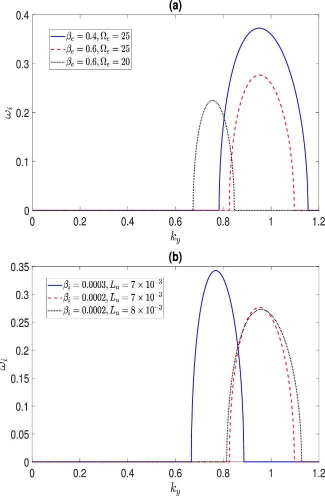
Figure 2. Classical plasmas with βe < 1. The profiles of the growth rates are shown with the variations of different plasma parameters as in the legends with m = 1900, Γ = 1.5 and $\tilde{g}=2.53\times 1{0}^{-16}$. The other fixed parameter values for subplots (a) and (b), respectively, are (Ln = 7 × 10⁻³ and βi = 0.0002) and (βe = 0.6 and Ωe = 25). |
3.1.2. Case II: βe > 1
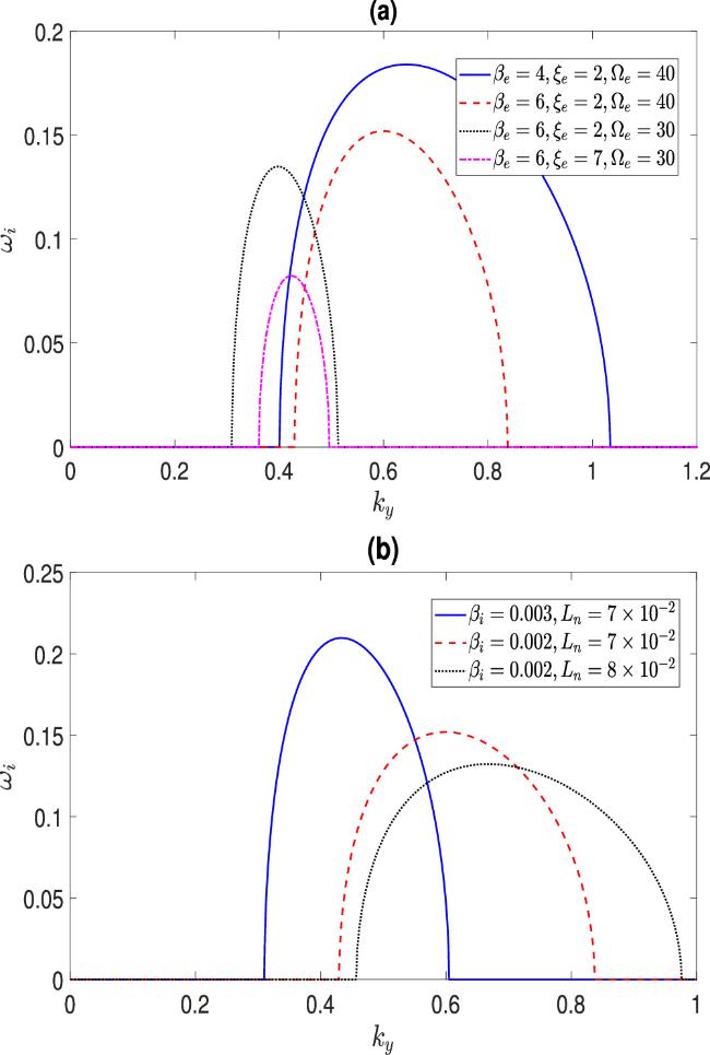
In the case of larger thermal energy than the rest mass energy of electrons, we choose the typical parametric values relevant for laboratory plasmas [39] as n0(0) ≃ 1015 − 1022cm−3, Ti ≃ 4.35 × 10⁷ − 4.35 × 10⁹ K, Te ≃ 1.18 × 10¹⁰ − 4.74 × 10¹⁰K, B0 ≃ 9.47 × 10⁴ − 2.99 × 10⁸G, g ≃ 102 − 108cm s−2, and Ln ≃ 6.83 × 10⁻⁶ − 7.2 × 10⁻¹cm. A reduction in the growth rate, similar to Case I, is also noted. However, the reduction becomes significant with increasing values of βe, and decreasing values of the magnetic field strength (Ωe) and the ion thermal energy (βi). Not only are the growth rates reduced like in Case I, but the instability domains also significantly shrink with increasing values of βe and βi but decreasing values of Ln. The results are displayed in figure 3. Also, similar to Case I, the instability domains shift towards lower (or higher) values of ky as the magnetic field strength decreases (or the length scale, Ln increases or the ion thermal energy decreases relative to the rest mass). Thus, it follows that although the qualitative features of the instability growth rates are similar, the instability growth rate is found to be higher in the case of βe < 1 compared to βe > 1 and the instability domains significantly differ in the two regimes of electron thermal energy. In particular, for βi ~ 0.0002, βe = 4, Ωe ~ 40, and Ln ~ 7 × 10⁻², the maximum growth rate is found to be ${\omega }_{i}^{\max }=0.18$ at ky = 0.51.
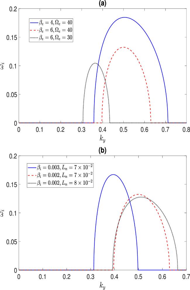
Figure 3. Classical plasmas with βe > 1. The profiles of the growth rates are shown with the variations of different plasma parameters as in the legends with m = 1900, Γ = 1.5, and $\tilde{g}=2.53\times 1{0}^{-16}$. The other fixed parameter values for subplots (a) and (b), respectively, are (Ln = 7 × 10⁻² and βi = 0.002) and (βe = 6 and Ωe = 40). |
3.2. Fully degenerate electrons
We consider the case in which electrons form a Fermi degenerate gas at zero temperature (Te = 0 K). In astrophysical environments, such as those in the core of massive stars like white dwarfs [10, 11], ions are typically nondegenerate, i.e., classical (Ti ≫ TFi) due to their inertia and electrons can be fully degenerate (Te ≪ TFe) providing the degeneracy pressure to prevent the collapse of the stars. Here, TFj denotes the Fermi temperature for j-th species particles. The Fermi–Dirac pressure law for degenerate electrons (at T = 0 K) gives [24, 40]26 ) can now be studied numerically for fully degenerate e-i plasmas. The results are displayed in figure 4. In this case, the expressions for Pe0(0) and b are given by
$\begin{eqnarray}{P}_{F}=\frac{{m}_{e}^{3}{c}^{3}}{8{\pi }^{2}{\hslash }^{3}{n}_{e0}(0)}\left[R{\left(1+{R}^{2}\right)}^{1/2}\left(\frac{2{R}^{2}}{3}-1\right)+{\sinh }^{-1}R\right],\end{eqnarray}$
where $R={R}_{0}(0){n}_{e}^{1/3}$ is the Fermi momentum normalized by mec with ${R}_{0}(0)=(\hslash /{m}_{e}c){\left(3{\pi }^{2}{n}_{e0}(0)\right)}^{1/3}$ denoting the degeneracy parameter and ℏ = h/2π the reduced Plank's constant. The normalized enthalpy of electrons is ${H}_{e}={n}_{e}\sqrt{1+{R}^{2}}$. Note that, the electron degeneracy can be highly relativistic if R ≫ 1 and non-relativistic if R ≪ 1. In fully degenerate e-i plasmas, the Fermi energy (kBTFe) is much higher than the thermal energy (kBTe) of electrons i.e., kBTFe ≫ kBTe and R0(0) measures the degree of degeneracy of unperturbed electrons. The general dispersion relation ( $\begin{eqnarray}\begin{array}{rcl}{P}_{e0}(0) & = & \frac{3}{8{R}_{0}^{3}(0)}\left[{R}_{0}(0){\left(1+{R}_{0}^{2}(0)\right)}^{1/2}\left(\frac{2{R}_{0}^{2}(0)}{3}-1\right)\right.\\ & & \left.+{\sinh }^{-1}{R}_{0}(0)\right],\end{array}\end{eqnarray}$
$\begin{eqnarray}b=\frac{1}{3}{R}_{0}^{2}(0){\left[1+{R}_{0}^{2}(0)\right]}^{-1/2}.\end{eqnarray}$
We choose the typical parametric values relevant for the environments of magnetized white dwarfs [10, 11] as: n0(0) ≃ 1030 − 1032 cm−3, Ti = 3.26 × 10⁶ − 3.26 × 10⁹K, B0 ≃ 7.48 × 10¹⁰ − 2.99 × 10¹³G, g ≃ 108cm s−2, and Ln ≃ 1.13 × 10⁻¹⁰ − 1.59 × 10⁻⁷ cm. From figure 4, we note that the qualitative features of the instability growth rate in fully degenerate plasmas are quite distinctive compared to the classical nondegenerate plasmas (cf. Figures 2 and 3). We also find that similar to figures 2 and 3, the instability growth rate is reduced but the instability domain expands due to the reduction of the ion thermal energy compared to the rest mass energy (see the dashed and dotted lines). Furthermore, while the magnetic field strength enhances the growth rate and the instability domain (see the blue solid line and dashed lines), the degeneracy parameter, in contrast, reduces both of them (see the dotted and dash-dotted lines). The latter is in agreement with the investigation [30] where the authors have shown that the quantum pressure can weaken the RTI in quantum plasmas. However, the growth rate can be reduced but the instability domain can be expanded by increasing the inhomogeneity scale size (see the dash-dotted and green solid lines). In particular, for βi ~ 0.003, R0(0) ~ 2, Ωe ~ 40, and Ln ~ 7 × 10⁻², the maximum growth rate is found to be ${\omega }_{i}^{\max }\approx 0.676$ at ky = 0.14. Thus, in comparison with the classical results, it may be concluded that the fully degenerate Fermi gas with higher relativistic degeneracy tends to weaken the RTI.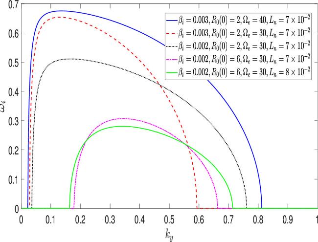
Figure 4. Fully degenerate plasmas: The profiles of the growth rates are shown with the variations of different plasma parameters as in the legends with m = 1900, Γ = 1.5, and $\tilde{g}=2.80\times 1{0}^{-21}$. |
3.3. Partially degenerate electrons
In many astrophysical situations (e.g., the environments of white dwarfs, neutron stars, and in gas giants like Jupiter) or laser produced plasmas, the strict condition Te ≪ TFe for full degeneracy of electrons may not always be fulfilled, i.e., there may not be any strict upper limit for the energy levels. Thus, one can reasonably assume either Te < TFe or Te > TFe. We, however, consider the regime where the electron Fermi energy is larger than the thermal energy, i.e., Te < TFe, the dimensionless electron chemical energy ξ = μ/kBTe is positive and finite, and the electron thermal and the rest mass energies do not differ significantly, i.e., βe ≡ kBTe/mec2 ~ 1 (implying that either βe < 1 or βe > 1). Thus, for partially degenerate electrons or electrons with arbitrary degeneracy, we consider the following expression for the electron number density [41, 42].38 ) can be put into the following alternative form [41, 43]
$\begin{eqnarray}{n}_{e}=\int f{\rm{d}}{p}_{e}=\frac{2}{{(2\pi \hslash )}^{3}}{\int }_{0}^{\infty }\frac{4\pi {p}_{e}^{2}}{\exp \left(\frac{E({p}_{e})-\mu }{{k}_{{\rm{B}}}{T}_{e}}\right)+1}{\rm{d}}{p}_{e},\end{eqnarray}$
where ℏ is the Planck's constant divided by 2π and μ is the chemical potential energy for electrons without the rest mass energy. Also, $E({p}_{e})=\sqrt{{c}^{2}{p}_{e}^{2}+{m}_{e}^{2}{c}^{4}}$ is the relativistic energy, and pe and me are, respectively, the relativistic momentum and the rest mass of electrons. Equation ( $\begin{eqnarray}{n}_{e}=\frac{8\pi \sqrt{2}}{{(2\pi \hslash )}^{3}}{m}_{e}^{3}{c}^{3}{\beta }_{e}^{3/2}\left[{F}_{1/2}(\xi ,{\beta }_{e})+{\beta }_{e}{F}_{3/2}(\xi ,{\beta }_{e})\right],\end{eqnarray}$
where Fk is the relativistic k-th order Fermi–Dirac integral, given by, $\begin{eqnarray}{F}_{k}(\xi ,{\beta }_{e})={\int }_{0}^{\infty }\frac{{\zeta }^{k}\sqrt{1+({\beta }_{e}/2)\zeta }}{1+\exp (\zeta -\xi )}{\rm{d}}\zeta ,\end{eqnarray}$
in which βe = kBTe/mec2 is the relativity parameter defined before, ζ = E(pe)/kBTe, and the normalized chemical potential energy ξ = μ/kBTe is called the electron degeneracy parameter.The electron degeneracy pressure at finite temperature (T ≠ 0K) is given by [41, 43]39 ) and following the method by Landau and Lifshitz [44], we obtain the following expressions for the dimensionless electron number density ne and the partially degenerate pressure Pe in two different cases of βe < 1 and βe > 1 as (see, for details, [45])
$\begin{eqnarray}{P}_{e}=\frac{1}{3{\pi }^{2}{\hslash }^{3}}{\int }_{0}^{\infty }\frac{{p}_{e}^{3}}{\exp \left(\frac{E({p}_{e})-\mu }{{k}_{{\rm{B}}}{T}_{e}}\right)+1}{\rm{d}}E,\end{eqnarray}$
which can be expressed as $\begin{eqnarray}{P}_{e}=\frac{{2}^{3/2}}{3{\pi }^{2}{\hslash }^{3}}{m}_{e}^{4}{c}^{5}{\beta }_{e}^{5/2}\left[{F}_{3/2}(\xi ,{\beta }_{e})+\frac{{\beta }_{e}}{2}{F}_{5/2}(\xi ,{\beta }_{e})\right].\end{eqnarray}$
Furthermore, ξ satisfies the following strict condition (without the relativistic and electrostatic potential energies) $\begin{eqnarray}{\sum }_{j=e,p}{\left[1+\exp \left(-\xi \right)\right]}^{-1}\leqslant 1.\end{eqnarray}$
Next, evaluating the integrals Fk(ξ, βe) in equation ( $\begin{eqnarray}{n}_{e}=\left\{\begin{array}{ll}{A}_{e}\left[\left\{{\xi }^{3/2}+\frac{{\pi }^{2}}{8}{\xi }^{-1/2}+\frac{7{\pi }^{4}}{640}{\xi }^{-5/2}\right\}+\frac{3{\beta }_{e}}{5}\left\{{\xi }^{5/2}+\frac{5{\pi }^{2}}{8}{\xi }^{1/2}-\frac{7{\pi }^{4}}{384}{\xi }^{-3/2}\right\}\right], & {\rm{for}}\,{\beta }_{e}\lt 1,\\ {A}_{e}\left[\left\{{\xi }^{2}+\frac{{\pi }^{2}}{3}\right\}+\frac{2{\beta }_{e}}{3}\left\{{\xi }^{3}+{\pi }^{2}\xi \right\}\right], & {\rm{for}}\,{\beta }_{e}\gt 1,\end{array}\right.\end{eqnarray}$
$\begin{eqnarray}{P}_{e}=\left\{\begin{array}{ll}\frac{2}{5}{\beta }_{e}{A}_{e}\left[\left\{{\xi }^{5/2}+\frac{5{\pi }^{2}}{8}{\xi }^{1/2}-\frac{7{\pi }^{4}}{384}{\xi }^{-3/2}\right\}+\frac{5{\beta }_{e}}{14}\left\{{\xi }^{7/2}+\frac{35{\pi }^{2}}{24}{\xi }^{3/2}+\frac{49{\pi }^{4}}{384}{\xi }^{-1/2}\right\}\right], & {\rm{for}}\,{\beta }_{e}\lt 1,\\ \frac{4}{9}{\beta }_{e}{A}_{e}\left[\left\{{\xi }^{3}+{\pi }^{2}\xi \right\}+\frac{3{\beta }_{e}}{8}\left\{{\xi }^{4}+2{\pi }^{2}{\xi }^{2}+\frac{7{\pi }^{4}}{15}\right\}\right], & {\rm{for}}\,{\beta }_{e}\gt 1,\end{array}\right.\end{eqnarray}$
where the coefficient Ae is given by $\begin{eqnarray}{A}_{e}=\left\{\begin{array}{ll}{\left[\left({\xi }_{0}^{3/2}+\frac{{\pi }^{2}}{8}{\xi }_{0}^{-1/2}+\frac{7{\pi }^{4}}{640}{\xi }_{0}^{-5/2}\right)+\frac{3{\beta }_{e}}{5}\left({\xi }_{0}^{5/2}+\frac{5{\pi }^{2}}{8}{\xi }_{0}^{1/2}-\frac{7{\pi }^{4}}{384}{\xi }_{0}^{-3/2}\right)\right]}^{-1}, & {\rm{for}}\,{\beta }_{j}\lt 1,\\ {\left[\left({\xi }_{0}^{2}+\frac{{\pi }^{2}}{3}\right)+\frac{2{\beta }_{e}}{3}\left({\xi }_{0}^{3}+{\pi }^{2}{\xi }_{0}\right)\right]}^{-1}, & {\rm{for}}\,{\beta }_{j}\gt 1.\end{array}\right.\end{eqnarray}$
The total energy density and the enthalpy for electrons are defined as ${{ \mathcal E }}_{e}\approx {n}_{e}\sqrt{{v}_{e}^{2}+1}$ and ${H}_{e}\equiv {n}_{e}\sqrt{{v}_{e}^{2}+1}+{P}_{e}$ so that at equilibrium, ${H}_{e0}(x)={n}_{e0}(x)(\sqrt{{v}_{e0}^{2}(x)+1}+{P}_{e0}(0))$, αe = He0(x)/ne0(x) ~ (1 + Pe0(0)). The expressions for Pe0(0) and b are $\begin{eqnarray}{P}_{e0}(0)=\left\{\begin{array}{ll}\frac{2}{5}{\beta }_{e}{A}_{e}\left[\left\{{\xi }_{0}^{5/2}+\frac{5{\pi }^{2}}{8}{\xi }_{0}^{1/2}-\frac{7{\pi }^{4}}{384}{\xi }_{0}^{-3/2}\right\}+\frac{5{\beta }_{e}}{14}\left\{{\xi }_{0}^{7/2}+\frac{35{\pi }^{2}}{24}{\xi }_{0}^{3/2}+\frac{49{\pi }^{4}}{384}{\xi }_{0}^{-1/2}\right\}\right], & {\rm{for}}\,{\beta }_{e}\lt 1,\\ \frac{4}{9}{\beta }_{e}{A}_{e}\left[\left\{{\xi }_{0}^{3}+{\pi }^{2}{\xi }_{0}\right\}+\frac{3{\beta }_{e}}{8}\left\{{\xi }_{0}^{4}+2{\pi }^{2}{\xi }_{0}^{2}+\frac{7{\pi }^{4}}{15}\right\}\right], & {\rm{for}}\,{\beta }_{e}\gt 1,\end{array}\right.\end{eqnarray}$
$\begin{eqnarray}b={P}_{e1}/{n}_{e1}\approx \left\{\begin{array}{ll}\frac{2{\beta }_{e}}{3}\frac{\left\{{\xi }_{0}^{3/2}+\frac{{\pi }^{2}}{8}{\xi }_{0}^{-1/2}\right\}+\frac{{\beta }_{e}}{2}\left\{{\xi }_{0}^{5/2}+\frac{5{\pi }^{2}}{8}{\xi }_{0}^{1/2}\right\}}{\left\{{\xi }_{0}^{1/2}-\frac{{\pi }^{2}}{24}{\xi }_{0}^{-3/2}\right\}+{\beta }_{e}\left\{{\xi }_{0}^{3/2}+\frac{{\pi }^{2}}{8}{\xi }_{0}^{-1/2}\right\}}, & {\rm{for}}\,{\beta }_{e}\lt 1,\\ \frac{2{\beta }_{e}}{3}\frac{\left\{{\xi }_{0}^{2}+\frac{{\pi }^{2}}{3}\right\}+\frac{{\beta }_{e}}{2}\left\{{\xi }_{0}^{3}+{\pi }^{2}{\xi }_{0}\right\}}{\left[{\xi }_{0}+{\beta }_{e}\{{\xi }_{0}^{2}+\frac{{\pi }^{2}}{3}\}\right]}, & {\rm{for}}\,{\beta }_{e}\gt 1.\end{array}\right.\end{eqnarray}$
Next, we study the RTI in two different cases, namely βe < 1 and βe > 1 as follows:
3.3.1. Case I: βe < 1
In this case, we consider the typical parametric values relevant for astrophysical plasmas [10, 11] as n0(0) ≃ 1029 − 1031 cm−3, Ti ≃ 1.08 × 10⁵ − 4.35 × 10⁹K, Te ≃ 1.78 × 10⁹ − 4.74 × 10⁹K, B0 ≃ 2.36 × 10⁹ − 2.24 × 10¹²G, g ≃ 108cm s−2, Ln ≃ 2.27 × 10⁻¹¹ − 4.5 × 10⁻¹⁰cm, and μ ≃ 1.63 × 10⁻⁷ − 1.31 × 10⁻⁶erg. The qualitative features of the growth rate of instability by the effects of βe, βi, ξe, Ωe, and Ln remain similar to the classical case (cf. Figure 2). However, the reduction of the growth rate and the expansion of the instability domain are noticeable with a small increment of the parameter βe and a decrement of βi. As before, the magnetic field strength increases both the growth rate and the instability domain. In comparison with the cases of classical (section 3.1 ) and fully degenerate (section 3.2 ) plasmas, an interesting and distinct feature is noted in the effects of ξe. As the latter is increased or the electron chemical potential energy is enhanced compared to the electron rest mass energy, the growth rate and the instability domains are significantly reduced [see subplot (a) of figure 5]. Physically, since an enhancement of the chemical energy corresponds to a decrement of the electron thermal energy, the drift velocities are reduced and so the perturbed E × B0-drift velocity can have an upward direction to move the plasma layer upward. This leads to a reduction of spikes in the plasma penetrating the lighter fluid (magnetic field), which supports the plasma, and consequently, the growth rate is reduced. Subplot (b) shows that similar to the cases of classical and fully degenerate electrons, not only are the growth rates significantly reduced, but the instability domains shift towards higher values of ky as βi is slightly reduced or the length scale of inhomogeneity Ln is increased. In particular, for βi ~ 0.0002, βe ~ 0.4, ξe ~ 2, Ωe ~ 25, and Ln ~ 7 × 10⁻³, the maximum growth rate can be observed as ${\omega }_{i}^{\max }=0.38$ at ky = 0.97.
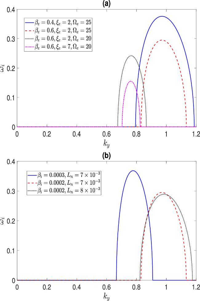
Figure 5. Partially degenerate plasmas with βe < 1. The profiles of the growth rates are shown with the variations of different plasma parameters as in the legends with m = 1900, Γ = 1.5 and $\tilde{g}=2.80\times 1{0}^{-21}$. The other fixed parameter values for subplots (a) and (b), respectively, are (Ln = 7 × 10⁻³ and βi = 0.0002) and (βe = 0.6, ξ = 2 and Ωe = 25). |
3.3.2. Case II: βe > 1
In the case of higher thermal energy than the rest mass energy of electrons, we choose the typical parametric values relevant for astrophysical plasmas [10, 11] as n0(0) ≃ 1030 − 1032 cm−3, Ti ≃ 1.08 × 10⁶ − 4.35 × 10¹⁰K, Te ≃ 1.78 × 10¹⁰ − 4.74 × 10¹⁰K, B0 ≃ 7.38 × 10⁹ − 4.11 × 10¹²G, g ≃ 108cm s−2, Ln ≃ 1.13 × 10⁻¹⁰ − 1.82 × 10⁻⁸cm, and μ ≃ 1.63 × 10⁻⁶ − 1.31 × 10⁻⁵erg. Here, a reduction of the growth rate is observed similar to Case I, however, in contrast to Case I, the instability domains get reduced with increasing values of βe > 1 and ξe. Also, similar to Case I, the growth rate is enhanced but the instability domain shrinks at increasing values of βi, and both are increased at increasing values of the magnetic field strength [see subplot (a) of figure 6]. Also, the growth rate of instability gets significantly reduced but the instability domain expands and shifts towards higher values of ky by the effects of the inhomogeneity length scale Ln [see subplot (b) of figure 6]. Thus, it may be concluded that higher electron chemical energy reduces the instability domain and the growth rate, i.e., the finite temperature degeneracy of electrons also tends to weaken the RTI. In particular, for βi ~ 0.002, ξe ~ 2, Ωe ~ 40, and Ln ~ 7 × 10⁻², the maximum growth rate is obtained as ${\omega }_{i}^{\max }=0.18$ at ky = 0.64.
Figure 6. Partially degenerate plasmas βe > 1. The profiles of the growth rates are shown with the variations of different plasma parameters as in the legends with m = 1900, Γ = 1.5 and $\tilde{g}=2.80\times 1{0}^{-21}$. The other fixed parameter values for subplots (a) and (b), respectively, are (Ln = 7 × 10⁻² and βi = 0.002) and (βe = 6, ξ = 2 and Ωe = 40). |
4. Conclusion
We have investigated the Rayleigh–Taylor instability of electrostatic perturbations in relativistic electron-ion magnetoplasmas under the influences of the unperturbed plasma density gradient and the constant gravity force. Specifically, we have focused on three different plasma regimes, namely, (i) when electrons are in isothermal equilibrium and follow the classical isothermal equation of state, (ii) electrons form a fully degenerate Fermi gas at zero temperature, and (iii) electrons are partially degenerate or have finite temperature degeneracy. Starting from a relativistic fluid model for electrons and ions and considering appropriate equations of state for classical and degenerate electrons, we have obtained the general dispersion relation, which we have analyzed in the three cases. In regimes of classical plasmas such as those in laboratory and magnetic confinement fusion plasmas, while the isothermal motion of electrons tends to reduce the instability growth rate, the ion thermal energy, and the external magnetic field enhance the RTI growth rate. Also, in regimes of higher electron thermal energy than its rest mass energy, the instability growth rate can be reduced with higher values of the length scale of density inhomogeneity than the ion plasma skin depth. In regimes of fully degenerate plasmas (or partially degenerate plasmas), such as those in the environments of massive white dwarf stars, the effect of the electron degeneracy pressure (or the electron chemical energy) is to reduce both the instability domain and the growth rate of RTI, implying that relativistic degeneracy or finite temperature degeneracy of electrons tends to suppress the RTI and a complete suppression may occur in the ultra-relativistic regime or in the regime of higher chemical energies than the rest mass energy. The prevention of such instabilities can lead to several important insights for understanding the underlying dynamics of RTIs.
In certain astrophysical plasmas, when the electron temperature drops below 109 K but higher than 107 K, electrons deviate from thermal and chemical equilibrium to form a partially degenerate gas, and, since they can strongly scatter with the plasma, their distributions can be governed by the Fermi–Dirac pressure law with the energy spectrum ranging from the thermal to Fermi energies. In these partially degenerate regimes, we have seen that higher chemical energy (than the thermal energy) and higher thermal energy (than the rest mass energy) of electrons are required to bring both the instability domain and the growth rate of RTI.
To conclude, the present theory should help understand the occurrence of RTI and the instability domains in a wide range of plasma environments ranging from laboratory to astrophysical settings where electrons can be in isothermal equilibrium and can deviate from the thermal and chemical equilibrium to form a partially degenerate or fully degenerate Fermi gas. In the present work, we have neglected the effects of fluid kinematic viscosity and particle collision. Such dissipative effects will certainly modify the instability criteria and can weaken the RTI growth. However, a detailed analysis is beyond the scope of the present work.