


1. Introduction
The study of nonlinear optical phenomena in nanoscale systems has attracted substantial interest due to their potential applications in photonic devices, sensing, and biomedical imaging [1–3]. Among these phenomena, second harmonic generation (SHG) is particularly significant, offering a pathway to convert low-frequency light into higher frequencies, thereby enabling various technological advancements [4–6]. Metallic nanoparticles (MNPs) are particularly attractive for enhancing SHG because of their unique plasmonic properties, which enable strong confinement and enhancement of electromagnetic fields at the nanoscale [7–10].
In 1961, for the first time, Franken et al [11] observed generation of second harmonics (SH) in quartz which was the first nonlinear phenomenon in the nonlinear optics. Its realization happened just after the appearance of the first laser by Maiman [12]. The problems of harmonics generation are investigated in several theoretical works, just as an example see [13–17].
The enhancement of SHG in MNPs is a subject of intensive research, as it bridges fundamental physics and practical applications. SHG in an individual NP has been studied extensively, revealing critical insights into the role of surface plasmons and local field enhancements [18–21]. However, recent studies have shifted focus towards the assemblies of NPs, where interparticle interactions can lead to significantly altered and often enhanced nonlinear optical responses [22–25].
NP trimers, consisting of three closely spaced NPs, represent a particularly fascinating system for studying these interactions due to their relatively simple yet sufficiently complex geometry [26–28]. The interactions in such systems can lead to complex electromagnetic coupling effects, modifying the optical properties and SHG efficiency in ways that are not observed in isolated NPs [29–34].
In this theoretical study, we aim to elucidate the mechanisms underlying SHG in an MNP trimer subjected to a laser beam radiation. By employing a classical electrodynamics framework, we analyze the nonlinear interactions between the laser beam fields and the NPs, taking into account dipole–dipole interactions among the particles [21, 25, 29, 35–39]. Through analytical derivation, we quantify the impact of these interactions on SHG for two distinct polarizations of the laser beam. Our findings are qualitatively in agreement with some experimental data [40, 41].
The results presented in this study contribute to a deeper understanding of the role of interparticle interactions in enhancing nonlinear optical processes in NP assemblies [42, 43]. These insights are crucial for the rational design of nanophotonic devices that leverage the unique properties of plasmonic NPs for advanced technological applications [44, 45]. The strength of interparticle interaction is extremely dependent on the distance of NPs which causes the dependence of linear and nonlinear properties of the NPs' arrangement on the average separation of particles. For example, the dependence of the extinction coefficient on the particles' separation can be used for measurement of the particles' distance in so-called plasmon nanoruler devices [6]. In another important application, for the detection of concentration of metal NPs, one can use maps of SH intensity [6]. However, the information about the dependence of SH radiation on interparticle interactions can give more proper estimations.
2. Model
In this study, we examine a trimer consisting of three identical spherical MNPs, each with a radius $a$ and separated by a distance $d$, subjected to electromagnetic radiation from a laser beam. Our analysis focuses exclusively on the dynamics of conduction electrons within each MNP, neglecting the role of ions in the interaction with the high-frequency electromagnetic fields of the incident laser beam. We assume that the laser beam is incident perpendicularly to the trimer axis, allowing us to distinguish between two possible polarizations of the electric field, as illustrated in figure 1: in case (a), the electric field is parallel to the trimer axis, while in case (b), it is perpendicular.
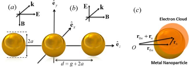
Figure 1. Configuration of the problem for two distinct scenarios: (a) the laser beam's electric field is aligned parallel to the trimer's symmetry axis, (b) the laser beam's magnetic field is aligned parallel to the trimer's symmetry axis, and (c) displacement of the conduction electron cloud from its initial equilibrium position shown only for one of the NPs, i.e. nth NP where n = 1, 2, 3. |
It should be mentioned that the model equations used here are similar to those that we have employed in our previous work for an MNP dimer [21], however we repeat some details here in order to avoid any confusion. Utilizing the rigid body approximation, we assume that all conduction electrons experience identical forces at any given moment, leading to uniform behavior among all electrons. This approximation holds true when the wavelength of the incident laser beam is significantly larger than the diameter of the NPs. The equation of motion for the conduction electrons in each MNP of the trimer can be expressed as follows:1 ) denotes the restoring force resulting from the displacement of electrons from their equilibrium state, with parameter $\xi $ being used to align the experimental data with the theoretical predictions. Under the ideal rigid body approximation, where all conduction electrons in the electronic cloud move uniformly, the value of $\xi $ is $1/3$. However, when considering real experimental data, $\xi $ is found to be less than $1/3$ and approaches zero for larger particles, reflecting the bulk medium characteristics. The electric field ${\boldsymbol{E}}({{\boldsymbol{r}}}_{0n}+{{\boldsymbol{r}}}_{{\boldsymbol{n}}},t)$ at the location of the nth MNP is the sum of the incident wave electric field ${{\boldsymbol{E}}}_{L}$ and the interaction term ${\sum }_{j\ne n}{{\boldsymbol{E}}}_{j\to n}$, which is induced by the electric dipole moments of the other NPs and it can be represented as
$\begin{eqnarray}\begin{array}{ccl}m\frac{{{\rm{d}}}^{2}{{\boldsymbol{r}}}_{n}}{{\rm{d}}{t}^{2}}+m\gamma \frac{{\rm{d}}{{\boldsymbol{r}}}_{n}}{{\rm{d}}t}+m\xi {\omega }_{p}^{2}{{\boldsymbol{r}}}_{n} & = & -e\left[{\boldsymbol{E}}\left({{\boldsymbol{r}}}_{0n}+{{\boldsymbol{r}}}_{n},t\right)+\frac{{\rm{d}}{{\boldsymbol{r}}}_{n}}{{\rm{d}}t}\right.\\ & & \left.{\rm{\times }}\,{\boldsymbol{B}}\left({{\boldsymbol{r}}}_{0n}+{{\boldsymbol{r}}}_{n},t\right)\right],n=1,2,3.\end{array}\end{eqnarray}$
Here, ${{\boldsymbol{r}}}_{0n}$, ${{\boldsymbol{r}}}_{n}$, $m$, $e$, $\gamma $, $\xi $ and ${\omega }_{p}$ represent the initial place of nth MNP, the displacement of the nth MNP conduction electron cloud from its initial equilibrium position, the electron mass, the magnitude of the electron charge, the damping coefficient, a function of the NP radius derived from experimental data, and the plasma frequency defined by the formula ${\omega }_{p}^{2}\,={n}_{0}{e}^{2}/{\varepsilon }_{0}m$, respectively. ${\varepsilon }_{0}$ is the vacuum permittivity, and ${n}_{0}$ is the equilibrium density of the electronic cloud. The third term on the left side of equation ( $\begin{eqnarray}\begin{array}{rcl}{\sum }_{j\ne n}{{\boldsymbol{E}}}_{j\to n} & = & \displaystyle \frac{1}{4\pi {\varepsilon }_{0}}\displaystyle \sum _{j\ne n}\left(\displaystyle \frac{{\boldsymbol{A}}}{{\left|{r}_{0n}-{r}_{0j}\right|}^{3}}\right.\\ & & \left.-\displaystyle \frac{{\rm{i}}k{\boldsymbol{A}}}{{\left|{r}_{0n}-{r}_{0j}\right|}^{2}}+\displaystyle \frac{{\boldsymbol{B}}}{\left|{r}_{0n}-{r}_{0j}\right|}\right),\end{array}\end{eqnarray}$
where $\begin{eqnarray}{\boldsymbol{A}}=3{\hat{{\boldsymbol{e}}}}_{j}\left({{\boldsymbol{p}}}_{j}.{\hat{{\boldsymbol{e}}}}_{j}\right)-{{\boldsymbol{p}}}_{j},{\boldsymbol{B}}={k}^{2}\left[{{\boldsymbol{p}}}_{j}-{\hat{{\boldsymbol{e}}}}_{j}\left({{\boldsymbol{p}}}_{j}.{\hat{{\boldsymbol{e}}}}_{j}\right)\right].\end{eqnarray}$
The normal vectors ${\hat{{\boldsymbol{e}}}}_{j}$ point from the center of the jth MNP toward the center of the nth MNP. The electric dipole moments of ${{\boldsymbol{p}}}_{j}$ are represented by ${{\boldsymbol{p}}}_{j}=-{Ze}{{\boldsymbol{r}}}_{j}$. Additionally, $Z=(4/3)\pi {a}^{3}{n}_{0}$ corresponds to the number of conduction electrons in each NP. To address the motion equation of electrons, we employ a well-established perturbative approach. In this framework, each parameter is expressed as a summation of different orders relative to the amplitude of the laser beam. $\begin{eqnarray}\begin{array}{rcl}{{\boldsymbol{r}}}_{i} & = & {{\boldsymbol{r}}}_{i}^{(1)}+{{\boldsymbol{r}}}_{i}^{(2)}+...,\\ {\boldsymbol{E}} & = & {{\boldsymbol{E}}}^{(1)}+{{\boldsymbol{E}}}^{(2)}+...,\\ {\boldsymbol{B}} & = & {{\boldsymbol{B}}}^{(1)}+{{\boldsymbol{B}}}^{(2)}+...,\,i=\mathrm{1,2}\,{\rm{and}}\,3.\end{array}\end{eqnarray}$
Given the small displacements of electronic clouds, denoted as ${{\boldsymbol{r}}}_{i}$, we can expand the fields using a Taylor series. Specifically, we write: $\begin{eqnarray}\begin{array}{ccc}{\boldsymbol{E}}({{\boldsymbol{r}}}_{0i}+{{\boldsymbol{r}}}_{i},t) & \,=\, & {{\boldsymbol{E}}}_{i}({{\boldsymbol{r}}}_{0i},t)+\displaystyle \sum _{l=1}^{\infty }\left({{\boldsymbol{r}}}_{i}^{(l)}.{\rm{\nabla }}\right){{\boldsymbol{E}}}_{i}({{\boldsymbol{r}}}_{0i},t)+...,\\ {{\boldsymbol{B}}}_{i}({{\boldsymbol{r}}}_{0i}+{{\boldsymbol{r}}}_{i},t) & = & \,{{\boldsymbol{B}}}_{i}({{\boldsymbol{r}}}_{0i},t)+\displaystyle \sum _{l=1}^{\infty }\left({{\boldsymbol{r}}}_{i}^{(l)}.{\rm{\nabla }}\right){{\boldsymbol{B}}}_{i}({{\boldsymbol{r}}}_{0i},t)+...,\\ & & i=1,2\,{\rm{and}}\,3.\end{array}\end{eqnarray}$
3. Parallel and perpendicular polarizations and fields inside an NP
When considering the normal incidence of a laser beam, we encounter two distinct cases regarding the orientation of the electric field: parallel to and perpendicular with the trimer axis. Each arbitrary case can be treated as a superposition of these modes. First, let's focus on parallel polarization. In this scenario, the laser beam's electric field aligns parallel to the orientation of the trimer axis, as depicted in figure 1(a) and it can be written as
$\begin{eqnarray}{{\boldsymbol{E}}}_{L,{||}}({\boldsymbol{r}},t)=\frac{1}{2}E{{\rm{e}}}^{{\rm{i}}({kx}-\omega t)}{\hat{{\boldsymbol{e}}}}_{z}+c.c.,\end{eqnarray}$
where $E$, $k$ and $\omega $ represent the amplitude, wavenumber and frequency of the incident wave, respectively, and $c.c.$ denotes the complex conjugate.Now, turning to the perpendicular case (as depicted in figure 1(b)), we assume that the laser electric field is perpendicular to the symmetry axis of the trimer. Specifically, we take the laser electric field as follows
$\begin{eqnarray}{{\boldsymbol{E}}}_{L,\perp }({\boldsymbol{r}},t)=\frac{1}{2}E{{\rm{e}}}^{{\rm{i}}({kx}-\omega t)}{\hat{{\boldsymbol{e}}}}_{y}+c.c..\end{eqnarray}$
For both cases (parallel and perpendicular), we can obtain the related magnetic field of the laser beam using Faraday's law. The expression for the magnetic field can be derived from the given equation ${\boldsymbol{k}}{\rm{\times }}{{\boldsymbol{E}}}_{L}=\omega {{\boldsymbol{B}}}_{L}$.In the context of electromagnetism, the electromagnetic fields of a laser beam inside an NP differ from their values in a vacuum. To address this, we adopt the standard approach commonly used in theoretical studies that describes the classical interaction of laser electromagnetic waves with NPs. Our first step involves determining the microscopic fields at the location of each individual MNP. We assume that the permittivity of the MNP is denoted as ${\varepsilon }_{n}$, while the ambient medium has a permittivity of ${\varepsilon }_{h}$. To analyze the situation where an external electric constant field $E$ exists in the presence of a spherical NP, we solve Laplace's equation with appropriate boundary conditions. This analysis yields the following results8 ), we obtain the electric field within the MNP as follows10 ), we observe that the microscopic electric field inside the MNP undergoes attenuation or amplification by a factor of
$\begin{eqnarray}{\phi }_{n}=-\left(\frac{3}{2+{\varepsilon }_{n}/{\varepsilon }_{h}}\right){Er}\cos \theta ,\end{eqnarray}$
$\begin{eqnarray}{\phi }_{h}=-{Er}\cos \theta +\left(\frac{{\varepsilon }_{n}/{\varepsilon }_{h}-1}{2+{\varepsilon }_{n}/{\varepsilon }_{h}}\right)\frac{{a}^{3}}{{r}^{2}}E\cos \theta ,\end{eqnarray}$
where ${\phi }_{n}$ and ${\phi }_{h}$ represent the electrostatic potentials inside and outside the MNP, respectively. Here, $r$ and $\theta $ denote the radial coordinate and azimuthal angle in the spherical coordinate system. By taking the gradient of the potential described by equation ( $\begin{eqnarray}{{\boldsymbol{E}}}_{{\boldsymbol{i}}}=\left(\frac{3}{2+{\varepsilon }_{n}/{\varepsilon }_{h}}\right){\boldsymbol{E}}.\end{eqnarray}$
Directly from equation ( $\begin{eqnarray}\alpha =\left(\frac{3}{2+{\varepsilon }_{n}/{\varepsilon }_{h}}\right).\end{eqnarray}$
4. Linear properties of an MNP trimer
For parallel polarization in the linear regime and for the first MNP, we can express the following relationship based on equation (1 )11 ), are considered to account for the variation of fields within the MNP. Similarly, two more equations can be formulated for the second and third MNPs. The solution to equation (12 ) has been previously derived in our earlier work [28], where we examined the linear properties of an MNP trimer. To ensure clarity, we provide a summary of the solution procedure here. By substituting equation (6 ) into equation (12 ) and considering the following interparticle interaction field term
$\begin{eqnarray}m\frac{{{\rm{d}}}^{2}{{\boldsymbol{r}}}_{1,{||}}^{(1)}}{{\rm{d}}{t}^{2}}+m\gamma \frac{{\rm{d}}{{\boldsymbol{r}}}_{1,{||}}^{(1)}}{{\rm{d}}{t}}+m\xi {\omega }_{p}^{2}{{\boldsymbol{r}}}_{1,{||}}^{(1)}=-e{{\boldsymbol{E}}}_{1,{||}}^{(1)},\end{eqnarray}$
where, ${{\boldsymbol{E}}}_{1,{||}}^{(1)}=\alpha {{\boldsymbol{E}}}_{L,{||}}+\alpha {{\boldsymbol{E}}}_{2\to 1,{||}}^{(1)}+\alpha {{\boldsymbol{E}}}_{3\to 1,{||}}^{(1)}$ and the coefficient $\alpha $, defined by equation ( $\begin{eqnarray}\begin{array}{ccc}\displaystyle \sum _{j=2}^{3}{{\boldsymbol{E}}}_{j\to 1,{\rm{||}}}^{(1)}({{\boldsymbol{r}}}_{01}) & = & \frac{-{Ze}}{2\pi {\varepsilon }_{0}}\displaystyle \sum _{j=2}^{3}\left(\frac{1}{{\left|(j-1)d\right|}^{3}}\right.\\ & & \left.-\frac{{\rm{i}}k}{{\left|(j-1)d\right|}^{2}}\right){{\boldsymbol{r}}}_{j,{\rm{||}}}^{(1)},\end{array}\end{eqnarray}$
and proposing periodic solutions of the form ${{\boldsymbol{r}}}_{n,{||}}^{(1)}\,=(1/2){\widetilde{r}}_{n,{||}}^{(1)}\exp [{\rm{i}}({kx}-\omega t)]{\hat{{\boldsymbol{e}}}}_{z}+c.c.$, where $n=1,2,3$ represents the amplitude of the electronic cloud displacement for each MNP, the amplitude can be directly derived as follows $\begin{eqnarray}{\widetilde{r}}_{1,{||}}^{(1)}={\widetilde{r}}_{3,{||}}^{(1)}=\left(\frac{1+{a}_{1}}{1-{a}_{2}-2{a}_{1}^{2}}\right){r}_{0},\end{eqnarray}$
$\begin{eqnarray}{\widetilde{r}}_{2,{||}}^{(1)}=\left(\frac{1+2{a}_{1}-{a}_{2}}{1-{a}_{2}-2{a}_{1}^{2}}\right){r}_{0},\end{eqnarray}$
where $\begin{eqnarray}{r}_{0}=\frac{\alpha {eE}}{m({\omega }^{2}+{\rm{i}}\omega \gamma -\xi {\omega }_{P}^{2})},\end{eqnarray}$
and $\begin{eqnarray}{a}_{1}=\frac{-\alpha Z{e}^{2}}{2\pi {\varepsilon }_{0}m({\omega }^{2}+{\rm{i}}\omega \gamma -\xi {\omega }_{P}^{2})}\left(\frac{1}{{d}^{3}}-\frac{{\rm{i}}k}{{d}^{2}}\right),\end{eqnarray}$
$\begin{eqnarray}{a}_{2}=\frac{-\alpha Z{e}^{2}}{2\pi {\varepsilon }_{0}m({\omega }^{2}+{\rm{i}}\omega \gamma -\xi {\omega }_{P}^{2})}\left(\frac{1}{8{d}^{3}}-\frac{{\rm{i}}k}{4{d}^{2}}\right).\end{eqnarray}$
Taking into account the linear displacement of the conduction electrons within the Drude model, we can readily derive the following expression for the permittivity of each MNP [28]: $\begin{eqnarray*}{\left(\frac{\varepsilon }{{\varepsilon }_{0}}\right)}_{1,{||}}={\left(\frac{\varepsilon }{{\varepsilon }_{0}}\right)}_{3,{||}}\end{eqnarray*}$
$\begin{eqnarray}=\,{\varepsilon }_{\infty }-\left(\frac{1+{a}_{1}}{1-{a}_{2}-2{a}_{1}^{2}}\right)\frac{{\omega }_{p}^{2}}{{\omega }^{2}+{\rm{i}}\omega \gamma -\xi {\omega }_{p}^{2}},\end{eqnarray}$
$\begin{eqnarray}{\left(\frac{\varepsilon }{{\varepsilon }_{0}}\right)}_{2,{||}}={\varepsilon }_{\infty }-\left(\frac{1+2{a}_{1}-{a}_{2}}{1-{a}_{2}-2{a}_{1}^{2}}\right)\frac{{\omega }_{p}^{2}}{{\omega }^{2}+{\rm{i}}\omega \gamma -\xi {\omega }_{p}^{2}}.\end{eqnarray}$
For further details, one can refer to our recent work [28].In the case where the electric field is perpendicular, the dipole electric fields of the second and third particles at the location of the first particle are given by [28],24 ) and (25 ) with their similar equations (17 ) and (18 ) of the parallel case of laser beam polarization, one can see that, here, there are some extra terms proportional to ${d}^{-1}$ originating from the term ${\boldsymbol{B}}$ in equation (3 ) used for the interparticle interactions. This term is proportional to ${{\boldsymbol{p}}}_{j}-{\hat{{\boldsymbol{e}}}}_{j}({{\boldsymbol{p}}}_{j}.{\hat{{\boldsymbol{e}}}}_{j})$ and for the parallel polarization case, it vanishes. As we will see in the numerical section, existence of such a term causes more intensive biparticle interactions which in turn, causes more intensive nonlinearity.
$\begin{eqnarray}\begin{array}{rcl}\displaystyle \sum _{j=2}^{3}{{\boldsymbol{E}}}_{j\to 1,\perp }^{\left(1\right)}\left({{\boldsymbol{r}}}_{01}\right) & = & \frac{{Ze}}{4\pi {\varepsilon }_{0}}\displaystyle \sum _{j=2}^{3}\left(\frac{1}{{\left|(j-1)d\right|}^{3}}\right.\\ & & -\frac{{\rm{i}}{k}}{{\left|(j-1)d\right|}^{2}}\left.-\frac{{k}^{2}}{\left|(j-1)d\right|}\right){{\boldsymbol{r}}}_{j,\perp }^{(1)}.\end{array}\end{eqnarray}$
For the perpendicular orientation of the laser electric field, using a similar approach and considering the displacement of each MNP as ${{\boldsymbol{r}}}_{n,\perp }^{(1)}=(1/2){\widetilde{r}}_{n,\perp }^{(1)}\exp [{\rm{i}}({kx}-\omega t)]{\hat{{\boldsymbol{e}}}}_{y}+c.c.$ and $n=1,2,3$, we can derive the displacement amplitudes as follows $\begin{eqnarray}{\widetilde{r}}_{1,\perp }^{(1)}={\widetilde{r}}_{3,\perp }^{(1)}=\left(\frac{1+{a}_{3}}{1-{a}_{4}-2{a}_{3}^{2}}\right){r}_{0},\end{eqnarray}$
$\begin{eqnarray}{\widetilde{r}}_{2,\perp }^{(1)}=\left(\frac{1+2{a}_{3}-{a}_{4}}{1-{a}_{4}-2{a}_{3}^{2}}\right){r}_{0},\end{eqnarray}$
where $\begin{eqnarray}{a}_{3}=\frac{\alpha Z{e}^{2}}{4\pi {\varepsilon }_{0}m({\omega }^{2}+{\rm{i}}\omega \gamma -\xi {\omega }_{P}^{2})}\left(\frac{1}{{d}^{3}}-\frac{{\rm{i}}{k}}{{d}^{2}}-\frac{{k}^{2}}{d}\right),\end{eqnarray}$
$\begin{eqnarray}{a}_{4}=\frac{\alpha Z{e}^{2}}{4\pi {\varepsilon }_{0}m({\omega }^{2}+{\rm{i}}\omega \gamma -\xi {\omega }_{P}^{2})}\left(\frac{1}{8{d}^{3}}-\frac{{\rm{i}}{k}}{4{d}^{2}}-\frac{{k}^{2}}{d}\right).\end{eqnarray}$
By comparing equations (The permittivity of each MNP under the perpendicular polarization of the incident laser beam is expressed as
$\begin{eqnarray*}{\left(\frac{\varepsilon }{{\varepsilon }_{0}}\right)}_{1,\perp }={\left(\frac{\varepsilon }{{\varepsilon }_{0}}\right)}_{3,\perp }\end{eqnarray*}$
$\begin{eqnarray}=\,{\varepsilon }_{{\rm{\infty }}}-\left(\frac{1+{a}_{3}}{1-{a}_{4}-2{a}_{3}^{2}}\right)\frac{{\omega }_{P}^{2}}{{\omega }^{2}+{\rm{i}}\omega \gamma -\xi {\omega }_{P}^{2}},\end{eqnarray}$
$\begin{eqnarray}{\left(\frac{\varepsilon }{{\varepsilon }_{0}}\right)}_{2,\perp }={\varepsilon }_{\infty }-\left(\frac{1+2{a}_{3}-{a}_{4}}{1-{a}_{4}-2{a}_{3}^{2}}\right)\frac{{\omega }_{P}^{2}}{{\omega }^{2}+{\rm{i}}\omega \gamma -\xi {\omega }_{P}^{2}}.\end{eqnarray}$
In both cases, in the non-interactional limit when $d\to \infty $, the amplitudes of the displacement converge to the trivial solution of a single MNP, given by $\begin{eqnarray}{\widetilde{r}}_{\rm{single}}^{(1)}={r}_{0},\end{eqnarray}$
which is in agreement with [37].For small values of ${a}_{i}$($i=1,2,3\,\rm{and}\,4$), by expanding the terms ${(1-{a}_{1}-2{a}_{1}^{2})}^{-1}$ and ${(1-{a}_{4}-2{a}_{3}^{2})}^{-1}$ with respect to ${a}_{i}$ and retaining only the linear terms of ${a}_{i}$ in equations (19 ), (20 ), (26 ) and (27 ), we obtain13 ) and (21 ). Notably, they share the same mathematical structure as the dipole fields.
$\begin{eqnarray}{\left(\frac{\varepsilon }{{\varepsilon }_{0}}\right)}_{{||},\perp }={\left(\frac{\varepsilon }{{\varepsilon }_{0}}\right)}_{\rm{single}}-{\left(\frac{{\rm{\Delta }}\varepsilon }{{\varepsilon }_{0}}\right)}_{\mathrm{int},{\rm{||}},\perp },\end{eqnarray}$
where the first term represents the relative permittivity of a single non-interacting MNP $\begin{eqnarray}{\left(\frac{\varepsilon }{{\varepsilon }_{0}}\right)}_{\rm{single}}={\varepsilon }_{\infty }-\frac{{\omega }_{P}^{2}}{{\omega }^{2}+{\rm{i}}\omega \gamma -\xi {\omega }_{P}^{2}},\end{eqnarray}$
and the second term represents the deviation arising from interactions which can be represented as $\begin{eqnarray}{\left(\frac{{\rm{\Delta }}\varepsilon }{{\varepsilon }_{0}}\right)}_{1,\mathrm{int},{\rm{||}}}={\left(\frac{{\rm{\Delta }}\varepsilon }{{\varepsilon }_{0}}\right)}_{3,\mathrm{int},{\rm{||}}}=\frac{({a}_{1}+{a}_{2}){\omega }_{P}^{2}}{{\omega }^{2}+{\rm{i}}\omega \gamma -\xi {\omega }_{P}^{2}},\end{eqnarray}$
$\begin{eqnarray}{\left(\frac{{\rm{\Delta }}\varepsilon }{{\varepsilon }_{0}}\right)}_{2,\mathrm{int},{\rm{||}}}=\frac{2{a}_{1}{\omega }_{P}^{2}}{{\omega }^{2}+{\rm{i}}\omega \gamma -\xi {\omega }_{P}^{2}},\end{eqnarray}$
$\begin{eqnarray}{\left(\frac{{\rm{\Delta }}\varepsilon }{{\varepsilon }_{0}}\right)}_{1,\mathrm{int},\perp }={\left(\frac{{\rm{\Delta }}\varepsilon }{{\varepsilon }_{0}}\right)}_{3,\mathrm{int},\perp }=\frac{({a}_{3}+{a}_{4}){\omega }_{P}^{2}}{{\omega }^{2}+{\rm{i}}\omega \gamma -\xi {\omega }_{P}^{2}},\end{eqnarray}$
$\begin{eqnarray}{\left(\frac{{\rm{\Delta }}\varepsilon }{{\varepsilon }_{0}}\right)}_{2,\mathrm{int},\perp }=\frac{2{a}_{3}{\omega }_{P}^{2}}{{\omega }^{2}+{\rm{i}}\omega \gamma -\xi {\omega }_{P}^{2}}.\end{eqnarray}$
Indeed, the parameters ${a}_{i}$($i=1,2,3\,\rm{and}\,4$) play a crucial role in capturing the interparticle interactions within the dynamics of the problem. These parameters are closely tied to the dipole interaction fields described by equations (5. Second-order nonlinear optical response of an MNP trimer
For the case of parallel polarization and for the first MNP, the second-order motion equation can be derived directly from equation (1 ).36 ) represent the electric field generated by the second-order electric dipole in the x-direction at the center of the MNP36 ) vanish. Finally, by incorporating equations (14 ), (15 ) and (37 ) into equation (35 ), we obtain
$\begin{eqnarray}m\frac{{{\rm{d}}}^{2}{{\boldsymbol{r}}}_{1,{||}}^{(2)}}{{\rm{d}}{t}^{2}}+m\gamma \frac{{\rm{d}}{{\boldsymbol{r}}}_{1,{||}}^{(2)}}{{\rm{d}}t}+m\xi {\omega }_{p}^{2}{{\boldsymbol{r}}}_{1,{||}}^{(2)}=-e\left({{\boldsymbol{E}}}_{1,{||}}^{(2)}+{{\boldsymbol{v}}}_{1,{||}}^{(1)}{\rm{\times }}{{\boldsymbol{B}}}_{1,{||}}^{(1)}\right),\end{eqnarray}$
where the term representing the second-order electric field is given by $\begin{eqnarray}\begin{array}{rcl}{{\boldsymbol{E}}}_{1,{||}}^{(2)} & = & \alpha [{{\boldsymbol{E}}}_{2\to 1,{||}}^{(2)}({{\boldsymbol{r}}}_{01})+{{\boldsymbol{E}}}_{3\to 1,{||}}^{(2)}({{\boldsymbol{r}}}_{01})+({{\boldsymbol{r}}}_{1,{||}}^{(1)}.{\rm{\\nabla }}){{\boldsymbol{E}}}_{L,{||}}^{(1)}({{\boldsymbol{r}}}_{01})\\ & & +({{\boldsymbol{r}}}_{1,{||}}^{(1)}.{\rm{\\nabla }}){{\boldsymbol{E}}}_{3\to 1,{||}}^{(1)}({{\boldsymbol{r}}}_{01})+({{\boldsymbol{r}}}_{1,{||}}^{(1)}.{\rm{\\nabla }}){{\boldsymbol{E}}}_{2\to 1,{||}}^{(1)}({{\boldsymbol{r}}}_{01})],\end{array}\end{eqnarray}$
where the first and second terms on the right-hand side of equation ( $\begin{eqnarray}\begin{array}{rcl}\displaystyle \sum _{j=2}^{3}{{\boldsymbol{E}}}_{j\to 1,{||}}^{(2)}({{\boldsymbol{r}}}_{01}) & = & \frac{{Ze}}{4\pi {\varepsilon }_{0}}\displaystyle \sum _{j=2}^{3}\left(\frac{1}{{\left|(j-1)d\right|}^{3}}\right.\\ & & \left.-\frac{2{\rm{i}}{k}}{{\left|(j-1)d\right|}^{2}}-\frac{4{k}^{2}}{\left|(j-1)d\right|}\right){\widetilde{r}}_{j,{||}}^{(2)}{\hat{{\boldsymbol{e}}}}_{x},\end{array}\end{eqnarray}$
and the remaining terms in equation ( $\begin{eqnarray}\begin{array}{ccc}\frac{{{\rm{d}}}^{2}{{\boldsymbol{r}}}_{1,{||}}^{(2)}}{{\rm{d}}{t}^{2}}+\gamma \frac{{\rm{d}}{{\boldsymbol{r}}}_{1,{||}}^{(2)}}{{\rm{d}}t}+\xi {\omega }_{p}^{2}{{\boldsymbol{r}}}_{1,{||}}^{(2)} & = & \frac{{\rm{i}}{ke}\alpha E}{4m}{\widetilde{r}}_{1,{||}}^{(1)}({{\rm{e}}}^{2{\rm{i}}({kx}-\omega t)}+c.c.){\hat{{\boldsymbol{e}}}}_{x}\\ & & -\frac{\alpha Z{e}^{2}}{4\pi {\varepsilon }_{0}m}\left(\frac{1}{{d}^{3}}-\frac{2{ik}}{{d}^{2}}-\frac{4{k}^{2}}{d}\right){{\boldsymbol{r}}}_{2,{||}}^{(2)}\\ & & -\frac{\alpha Z{e}^{2}}{4\pi {\varepsilon }_{0}m}\left(\frac{1}{8{d}^{3}}-\frac{2{ik}}{4{d}^{2}}-\frac{4{k}^{2}}{2d}\right){{\boldsymbol{r}}}_{3,{||}}^{(2)}.\end{array}\end{eqnarray}$
Similarly, the equations describing the displacement of the electronic cloud for the second and third NPs can be written as follows $\begin{eqnarray}\begin{array}{ccc}\frac{{{\rm{d}}}^{2}{{\boldsymbol{r}}}_{2,{||}}^{(2)}}{{\rm{d}}{t}^{2}}+\gamma \frac{{\rm{d}}{{\boldsymbol{r}}}_{2,{||}}^{(2)}}{{\rm{d}}t}+\xi {\omega }_{p}^{2}{{\boldsymbol{r}}}_{2,{||}}^{(2)} & = & \frac{{\rm{i}}{ke}\alpha E}{4m}{\widetilde{r}}_{2,{||}}^{(1)}({{\rm{e}}}^{2{\rm{i}}({kx}-\omega t)}+c.c.){\hat{{\boldsymbol{e}}}}_{x}\\ & & -\frac{\alpha Z{e}^{2}}{4\pi {\varepsilon }_{0}m}\left(\frac{1}{{d}^{3}}-\frac{2{ik}}{{d}^{2}}-\frac{4{k}^{2}}{d}\right){{\boldsymbol{r}}}_{1,{||}}^{(2)}\\ & & -\frac{\alpha Z{e}^{2}}{4\pi {\varepsilon }_{0}m}\left(\frac{1}{{d}^{3}}-\frac{2{ik}}{{d}^{2}}-\frac{4{k}^{2}}{d}\right){{\boldsymbol{r}}}_{3,{||}}^{(2)},\end{array}\end{eqnarray}$
$\begin{eqnarray}\begin{array}{ccc}\frac{{{\rm{d}}}^{2}{{\boldsymbol{r}}}_{3,{\rm{||}}}^{(2)}}{{\rm{d}}{t}^{2}}+\gamma \frac{{\rm{d}}{{\boldsymbol{r}}}_{3,{\rm{||}}}^{(2)}}{{\rm{d}}t}+\xi {\omega }_{p}^{2}{{\boldsymbol{r}}}_{3,{\rm{||}}}^{(2)} & = & \frac{{\rm{i}}{ke}\alpha E}{4m}{\widetilde{r}}_{3,{\rm{||}}}^{(1)}({{\rm{e}}}^{2{\rm{i}}({kx}-\omega t)}+c.c.){\hat{{\boldsymbol{e}}}}_{x}\\ & & -\frac{\alpha Z{e}^{2}}{4\pi {\varepsilon }_{0}m}\left(\frac{1}{{d}^{3}}-\frac{2{ik}}{{d}^{2}}-\frac{4{k}^{2}}{d}\right){{\boldsymbol{r}}}_{2,{\rm{||}}}^{(2)}\\ & & -\frac{\alpha Z{e}^{2}}{4\pi {\varepsilon }_{0}m}\left(\frac{1}{8{d}^{3}}-\frac{2{ik}}{4{d}^{2}}-\frac{4{k}^{2}}{2d}\right){{\boldsymbol{r}}}_{1,{\rm{||}}}^{(2)}.\end{array}\end{eqnarray}$
Considering the following solutions38 )–(40 ), the second-order amplitudes can be readily obtained as
$\begin{eqnarray}{{\boldsymbol{r}}}_{i,||}^{(2)}=\frac{1}{2}{\tilde{r}}_{i,||}^{(2)}{{\rm{e}}}^{2{\rm{i}}({kx}-\omega t)}{\hat{{\boldsymbol{e}}}}_{x}+c.c.,\,i=1,2\,\rm{and}\,3,\end{eqnarray}$
in equations ( $\begin{eqnarray}\begin{array}{rcl}{\widetilde{r}}_{1,{||}}^{(2)} & = & {\widetilde{r}}_{3,{||}}^{(2)}=\frac{1+{a}_{1}+{a}_{5}+2{a}_{1}{a}_{5}-{a}_{2}{a}_{5}}{(1-2{a}_{1}^{2}-{a}_{2})(1-2{a}_{5}^{2}-{a}_{6})}\\ & & {\rm{\times }}\,\frac{-{ike}\alpha E}{2m(4{\omega }^{2}+2i\omega \gamma -\xi {\omega }_{p}^{2})}{r}_{0},\end{array}\end{eqnarray}$
$\begin{eqnarray}\begin{array}{rcl}{\widetilde{r}}_{2,{||}}^{(2)} & = & \frac{(1-{a}_{6})(1+2{a}_{1}-{a}_{2})-2{a}_{5}(1+{a}_{1})}{(1-2{a}_{1}^{2}-{a}_{2})(1-2{a}_{5}^{2}-{a}_{6})}\\ & & {\rm{\times }}\frac{-{ike}\alpha E}{2m(4{\omega }^{2}+2i\omega \gamma -\xi {\omega }_{p}^{2})}{r}_{0},\end{array}\end{eqnarray}$
where $\begin{eqnarray}{a}_{5}=\frac{\alpha Z{e}^{2}}{4\pi {\varepsilon }_{0}m(4{\omega }^{2}+2i\omega \gamma -\xi {\omega }_{p}^{2})}\left(\frac{1}{{d}^{3}}-\frac{2{ik}}{{d}^{2}}-\frac{4{k}^{2}}{d}\right),\end{eqnarray}$
$\begin{eqnarray}{a}_{6}=\frac{\alpha Z{e}^{2}}{4\pi {\varepsilon }_{0}m(4{\omega }^{2}+2i\omega \gamma -\xi {\omega }_{p}^{2})}\left(\frac{1}{8{d}^{3}}-\frac{2{ik}}{4{d}^{2}}-\frac{4{k}^{2}}{2d}\right).\end{eqnarray}$
Similarly, for the case of perpendicular polarization, we can obtain $\begin{eqnarray}{{\boldsymbol{r}}}_{i,\perp }^{(2)}=\frac{1}{2}{\tilde{r}}_{i,\perp }^{(2)}{{\rm{e}}}^{2{\rm{i}}({kx}-\omega t)}{\hat{{\boldsymbol{e}}}}_{x}+c.c.,i=1,2\,\rm{and}\,3,\end{eqnarray}$
where $\begin{eqnarray}\begin{array}{rcl}{\widetilde{r}}_{1,\perp }^{(2)} & = & {\widetilde{r}}_{3,\perp }^{(2)}=\frac{1+{a}_{3}+{a}_{5}+2{a}_{3}{a}_{5}-{a}_{4}{a}_{5}}{(1-2{a}_{3}^{2}-{a}_{4})(1-2{a}_{5}^{2}-{a}_{6})}\\ & & {\rm{\times }}\,\frac{-{ike}\alpha E}{2m(4{\omega }^{2}+2i\omega \gamma -\xi {\omega }_{p}^{2})}{r}_{0},\end{array}\end{eqnarray}$
$\begin{eqnarray}\begin{array}{rcl}{\widetilde{r}}_{2,\perp }^{(2)} & = & \frac{(1-{a}_{6})(1+2{a}_{3}-{a}_{4})-2{a}_{5}(1+{a}_{3})}{(1-2{a}_{1}^{2}-{a}_{2})(1-2{a}_{5}^{2}-{a}_{6})}\\ & & {\rm{\times }}\,\frac{-{ike}\alpha E}{2m(4{\omega }^{2}+2i\omega \gamma -\xi {\omega }_{p}^{2})}{r}_{0}.\end{array}\end{eqnarray}$
In the non-interactional approximation (i.e., $d\to \infty $), we can obtain the amplitudes of the displacements of a single MNP as follows $\begin{eqnarray}{\widetilde{r}}_{\rm{single}}^{(2)}=\frac{-{\rm{i}}{ke}\alpha E}{2m(4{\omega }^{2}+2i\omega \gamma -\xi {\omega }_{p}^{2})}{r}_{0}.\end{eqnarray}$
6. Second harmonics generation
To assess the impact of nonlinear interactions on the SHG of each particle, it is necessary to compute the second-order electric dipole moment of each MNP as follows ${\widetilde{p}}_{i}^{(2)}\,=-{Ze}{\widetilde{r}}_{i}^{(2)},i=1,2,3$.
The time-averaged power of the SH radiation per unit solid angle, emitted by the oscillating second-order electric dipole moment, can be expressed as [28]52 )–(55 ) as follows56 )–(59 ), we can expand the terms ${\left[(1-2{a}_{1}^{2}-{a}_{2})(1-2{a}_{5}^{2}-{a}_{6})\right]}^{-1}$ and $[(1-2{a}_{3}^{2}-{a}_{4}){(1-2{a}_{5}^{2}-{a}_{6})]}^{-1}$, with respect to these small parameters to get the following approximate relations60 )–(63 ), the contribution of inter-particle dipole–dipole interactions can be separated from the non-interacting particle radiation power, resulting in the expression for ${{\rm{\Pi }}}_{{||},\perp }^{(2)}={{\rm{\Pi }}}_{\rm{Single}}+{{\rm{\Pi }}}_{\mathrm{int},||,\perp }^{(2)}$, which is given by
$\begin{eqnarray}\frac{d{{\rm{\Pi }}}^{(2)}}{{\rm{d}}{\rm{\Omega }}}=\frac{{c}^{2}{Z}_{0}{k}^{4}}{32{\pi }^{2}}{\left|{p}^{(2)}\right|}^{2}{\sin }^{2}\theta ,\end{eqnarray}$
where ${Z}_{0}=\sqrt{{\mu }_{0}/{\varepsilon }_{0}}=376.730{\rm{\Omega }}$ is the impedance of the vacuum and $c$ is the speed of light in the vacuum. After integrating with respect to the solid angle ${\rm{\Omega }}$, the total radiated power can be obtained as $\begin{eqnarray}{{\rm{\Pi }}}^{(2)}=\frac{{c}^{2}{Z}_{0}{k}^{4}}{12\pi }{\left|{p}^{(2)}\right|}^{2}.\end{eqnarray}$
Consequently, the total SH power of each NP for parallel and perpendicular polarizations is as follows $\begin{eqnarray}\begin{array}{rcl}{{\rm{\Pi }}}_{1,{||}}^{(2)} & \,= & {{\rm{\Pi }}}_{3,{||}}^{(2)}=\frac{{c}^{2}{Z}_{0}{k}^{4}{Z}^{2}{e}^{2}}{12\pi }\\ & & {\rm{\times }}\,{\left|\frac{1+{a}_{1}+{a}_{5}+2{a}_{1}{a}_{5}-{a}_{2}{a}_{5}}{(1-2{a}_{1}^{2}-{a}_{2})(1-2{a}_{5}^{2}-{a}_{6})}{\widetilde{r}}_{{\rm{single}}}^{(2)}\right|}^{2},\end{array}\end{eqnarray}$
$\begin{eqnarray}\begin{array}{rcl}{\,{\rm{\Pi }}}_{2,{||}}^{(2)} & \,= & \frac{{c}^{2}{Z}_{0}{k}^{4}{Z}^{2}{e}^{2}}{12\pi }\\ & & {\rm{\times }}\,{\left|\frac{(1-{a}_{6})(1+2{a}_{1}-{a}_{2})-2{a}_{5}(1+{a}_{1})}{(1-2{a}_{1}^{2}-{a}_{2})(1-2{a}_{5}^{2}-{a}_{6})}{\widetilde{r}}_{{\rm{single}}}^{(2)}\right|}^{2},\end{array}\end{eqnarray}$
$\begin{eqnarray}\begin{array}{rcl}{{\rm{\Pi }}}_{1,\perp }^{(2)} & = & {{\rm{\Pi }}}_{2,\perp }^{(2)}=\frac{{c}^{2}{Z}_{0}{k}^{4}{Z}^{2}{e}^{2}}{12\pi }\\ & & {\rm{\times }}\,{\left|\frac{1+{a}_{3}+{a}_{5}+2{a}_{3}{a}_{5}-{a}_{4}{a}_{5}}{(1-2{a}_{3}^{2}-{a}_{4})(1-2{a}_{5}^{2}-{a}_{6})}{\widetilde{r}}_{\rm{single}}^{(2)}\right|}^{2},\end{array}\end{eqnarray}$
$\begin{eqnarray}\begin{array}{rcl}{\,{\rm{\Pi }}}_{2,\perp }^{\left(2\right)} & \,= & \frac{{c}^{2}{Z}_{0}{k}^{4}{Z}^{2}{e}^{2}}{12\pi }\\ & & {\rm{\times }}\,{\left|\frac{\left(1-{a}_{6}\right)\left(1+2{a}_{3}-{a}_{4}\right)-2{a}_{5}\left(1+{a}_{3}\right)}{\left(1-2{a}_{1}^{2}-{a}_{2}\right)\left(1-2{a}_{5}^{2}-{a}_{6}\right)}{\widetilde{r}}_{\rm{single}}^{\left(2\right)}\right|}^{2}.\end{array}\end{eqnarray}$
If we denote the radiated power of a single NP as ${{\rm{\Pi }}}_{\rm{Single}}^{(2)}\,={c}^{2}{Z}_{0}{k}^{4}{Z}^{2}{e}^{2}{\left|{\widetilde{r}}_{\rm{Single}}\right|}^{2}/12\pi $, we can rewrite equations ( $\begin{eqnarray}{{\rm{\Pi }}}_{1,{||}}^{(2)}={{\rm{\Pi }}}_{3,{||}}^{(2)}={\left|\frac{1+{a}_{1}+{a}_{5}+2{a}_{1}{a}_{5}-{a}_{2}{a}_{5}}{(1-2{a}_{1}^{2}-{a}_{2})(1-2{a}_{5}^{2}-{a}_{6})}\right|}^{2}{{\rm{\Pi }}}_{\rm{Single}}^{(2)},\end{eqnarray}$
$\begin{eqnarray}{{\rm{\Pi }}}_{2,{||}}^{(2)}={\left|\frac{(1-{a}_{6})(1+2{a}_{1}-{a}_{2})-2{a}_{5}(1+{a}_{1})}{(1-2{a}_{1}^{2}-{a}_{2})(1-2{a}_{5}^{2}-{a}_{6})}\right|}^{2}{{\rm{\Pi }}}_{\rm{Single}}^{(2)},\end{eqnarray}$
$\begin{eqnarray}{{\rm{\Pi }}}_{1,\perp }^{(2)}={{\rm{\Pi }}}_{2,\perp }^{(2)}={\left|\frac{1+{a}_{3}+{a}_{5}+2{a}_{3}{a}_{5}-{a}_{4}{a}_{5}}{(1-2{a}_{3}^{2}-{a}_{4})(1-2{a}_{5}^{2}-{a}_{6})}\right|}^{2}{{\rm{\Pi }}}_{\rm{Single}}^{(2)},\end{eqnarray}$
$\begin{eqnarray}{{\rm{\Pi }}}_{2,\perp }^{(2)}={\left|\frac{(1-{a}_{6})(1+2{a}_{3}-{a}_{4})-2{a}_{5}(1+{a}_{3})}{(1-2{a}_{3}^{2}-{a}_{4})(1-2{a}_{5}^{2}-{a}_{6})}\right|}^{2}{{\rm{\Pi }}}_{\rm{Single}}^{(2)}.\end{eqnarray}$
Considering the smallness of p`arameters $\left|{a}_{i}\right|$ where $i=\mathrm{1,2},...,6$, in equations ( $\begin{eqnarray}{{\rm{\Pi }}}_{1,{\rm{||}}}^{(2)}={{\rm{\Pi }}}_{3,{\rm{||}}}^{(2)}{\rm{\approx }}{{\rm{\Pi }}}_{\rm{single}}^{(2)}+2\mathrm{Re}({a}_{1}+{a}_{2}+{a}_{5}+{a}_{6}){{\rm{\Pi }}}_{\rm{single}}^{(2)},\end{eqnarray}$
$\begin{eqnarray}{{\rm{\Pi }}}_{2,{\rm{||}}}^{(2)}{\rm{\approx }}{{\rm{\Pi }}}_{\rm{single}}^{(2)}+2\mathrm{Re}(2{a}_{1}-2{a}_{5}){{\rm{\Pi }}}_{\rm{single}}^{(2)},\end{eqnarray}$
$\begin{eqnarray}{{\rm{\Pi }}}_{1,\perp }^{(2)}={{\rm{\Pi }}}_{3,\perp }^{(2)}{\rm{\approx }}{{\rm{\Pi }}}_{\rm{single}}^{(2)}+2\mathrm{Re}({a}_{3}+{a}_{4}+{a}_{5}+{a}_{6}){{\rm{\Pi }}}_{\rm{single}}^{(2)},\end{eqnarray}$
$\begin{eqnarray}{{\rm{\Pi }}}_{2,\perp }^{(2)}{\rm{\approx }}{{\rm{\Pi }}}_{\rm{single}}^{(2)}+2\mathrm{Re}(2{a}_{3}-2{a}_{5}){{\rm{\Pi }}}_{\rm{single}}^{(2)}.\end{eqnarray}$
From equations ( $\begin{eqnarray}{{\rm{\Pi }}}_{1,\mathrm{int},{\rm{||}}}^{(2)}={{\rm{\Pi }}}_{3,\mathrm{int},{\rm{||}}}^{(2)}=2\mathrm{Re}({a}_{1}+{a}_{2}+{a}_{5}+{a}_{6}){{\rm{\Pi }}}_{\rm{single}}^{(2)},\end{eqnarray}$
$\begin{eqnarray}{{\rm{\Pi }}}_{2,\mathrm{int},{\rm{||}}}^{(2)}=2\mathrm{Re}(2{a}_{1}-2{a}_{5}){{\rm{\Pi }}}_{\rm{single}}^{(2)},\end{eqnarray}$
$\begin{eqnarray}{{\rm{\Pi }}}_{1,\mathrm{int},\perp }^{(2)}={{\rm{\Pi }}}_{3,\mathrm{int},\perp }^{(2)}=2\mathrm{Re}({a}_{3}+{a}_{4}+{a}_{5}+{a}_{6}){{\rm{\Pi }}}_{\rm{single}}^{(2)},\end{eqnarray}$
$\begin{eqnarray}{{\rm{\Pi }}}_{2,\mathrm{int},\perp }^{(2)}=2\mathrm{Re}(2{a}_{3}-2{a}_{5}){{\rm{\Pi }}}_{\rm{single}}^{(2)}.\end{eqnarray}$
7. Numerical discussion
For the numerical analysis, we select gold NPs with diameters of 4 nm and 20 nm which are located in a glass medium. The parameters $\xi $, $\gamma $, ${\varepsilon }_{\infty }$ and ${\omega }_{p}$, which are necessary for calculating permittivity as specified in equations (19 )–(20 ) and (26 )–(27 ), are obtained from [37] and for avoiding any confusion we brought their values again in the appendix section.
In figure 2(a), for the parallel case of the incident electric field, we have plotted the variations of SH total radiated power versus incident laser beam wavelength, for each NP of trimer, when the radius of the NPs is $a=2\rm{nm}$ and the gap between the NPs is $g=2a=4\,\rm{nm}$. For comparison, we have plotted the curve for the non-interactional case or single NP and dimer with the similar geometry of the trimer, as well. Here, we normalized the curves with the maximum of the single particle radiation power. Because of the symmetry, the first and final NPs behave in the same manner. For all NPs, dipolar interparticle interaction causes the increase in the SH radiated power and the red-shift of the plasmon resonance peak. Here, for the middle NP, we have an increase of approximately 50% in the peak power with respect to the single NP radiation. Considering our previous work related to the linear properties of the metal trimer [28], the displacement of the plasmon peak wavelength in this nonlinear phenomenon is less than the peak displacement for the linear phenomenon of light scattering, however the same dynamics are maintained. The effect of the dipole interaction on the middle NP is more intensive, as one could expect, because it has the minimum distance from both NPs. For the single NP, the peak of the SH radiation power approximately coincides with the plasmon peak power of the extinction coefficient [37]. With a little distance, below the curve of the middle NP, the associated curve of the dimer is located. In figure 2(b), we have demonstrated the SH total power versus the incident laser beam wavelength for the second configuration case, when the laser magnetic field is parallel to the trimer axis, taking the same parameters of figure 2(a). For this case, the interaction causes the decrease in the SH radiation power and the blue-shift of the plasmon peak. For all NPs, the curves approximately coincide each other. These dynamics are also in accordance with the linear behavior of the system. The origin of the different behaviors of the two configuration modes return to the term ${{\boldsymbol{p}}}_{j}^{(2)}.{\hat{{\boldsymbol{e}}}}_{j}$ in the interactional electric field in equation (37 ). For the parallel magnetic case, this term vanishes and the interparticle interaction is weaker than the first case. It is better to mention that such dynamics are revealed for the dimer's SH radiation in some experimental [41] and theoretical [21] works, where the interaction causes the enhancement and red-shift of the plasmon peak of SH radiation for the parallel polarization of the incident laser beam and, inversely, its reduction and blue-shift for the perpendicular polarization. In this case, the curve of the dimer's SH radiation power is located under the single particle's one and above the trimer's one.
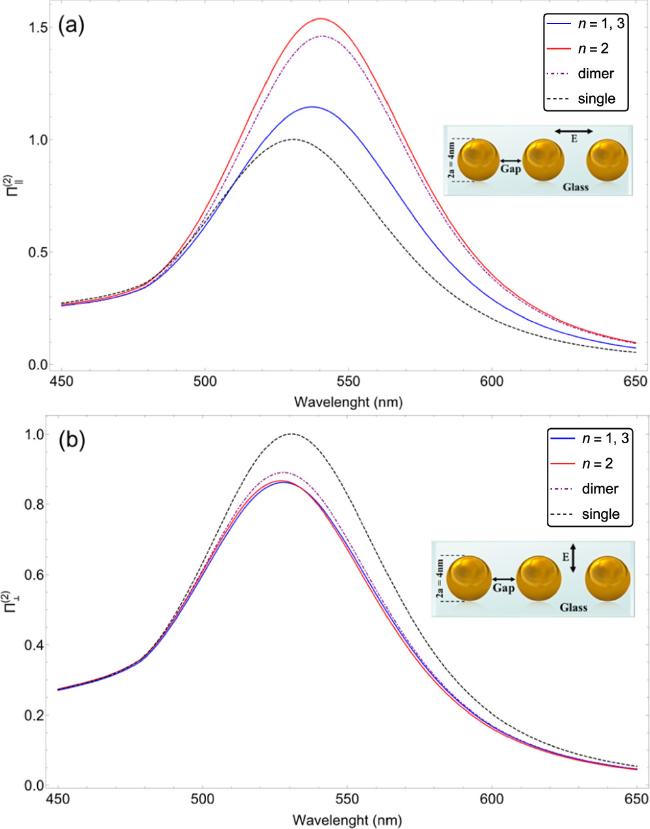
Figure 2. The total power radiation of the SH for (a) parallel and (b) perpendicular laser beam polarizations when the NP diameter is 2a = 4 nm and the gap distance is g = 2a. Here, n=1, 2, 3 indicate the first, second and third NP, respectively. |
In figure 3(a), for the case of the parallel laser beam electric field, we select larger NPs with a radius of $a=10{\rm{nm}}$ and set the other parameters as the former cases. It is clear that the increase in the size of the NPs' cases also increase the number of conduction electrons and consequently increase the induced electric dipoles, which in turn leads to more intensive interparticle interactions, resulting in, for all NPs, an increase in the SH radiated power approximately three times greater than the similar case with a smaller radius, i.e. Figure 2(a), and the same dynamics repeat again. In figure 3(b), for the parallel laser beam magnetic field case and for the larger NPs of $a=10{\rm{nm}}$, we have the SH power versus wavelength. Here, again, the increase in the size of the NPs causes a more intensive interparticle interaction. Here, deference between the radiation powers of the middle
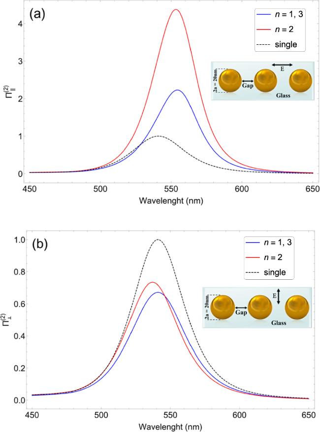
Figure 3. The total power radiation of the SH for (a) parallel and (b) perpendicular laser beam polarizations when the NP diameter is 2a = 20 nm and the gap distance is g = 2a. Here, n=1, 2, 3 indicates the first, second and third NP, respectively. |
and terminal NPs are evidence. Terminal NPs experience more reduction in the SH radiation power but less peak power red-shift.
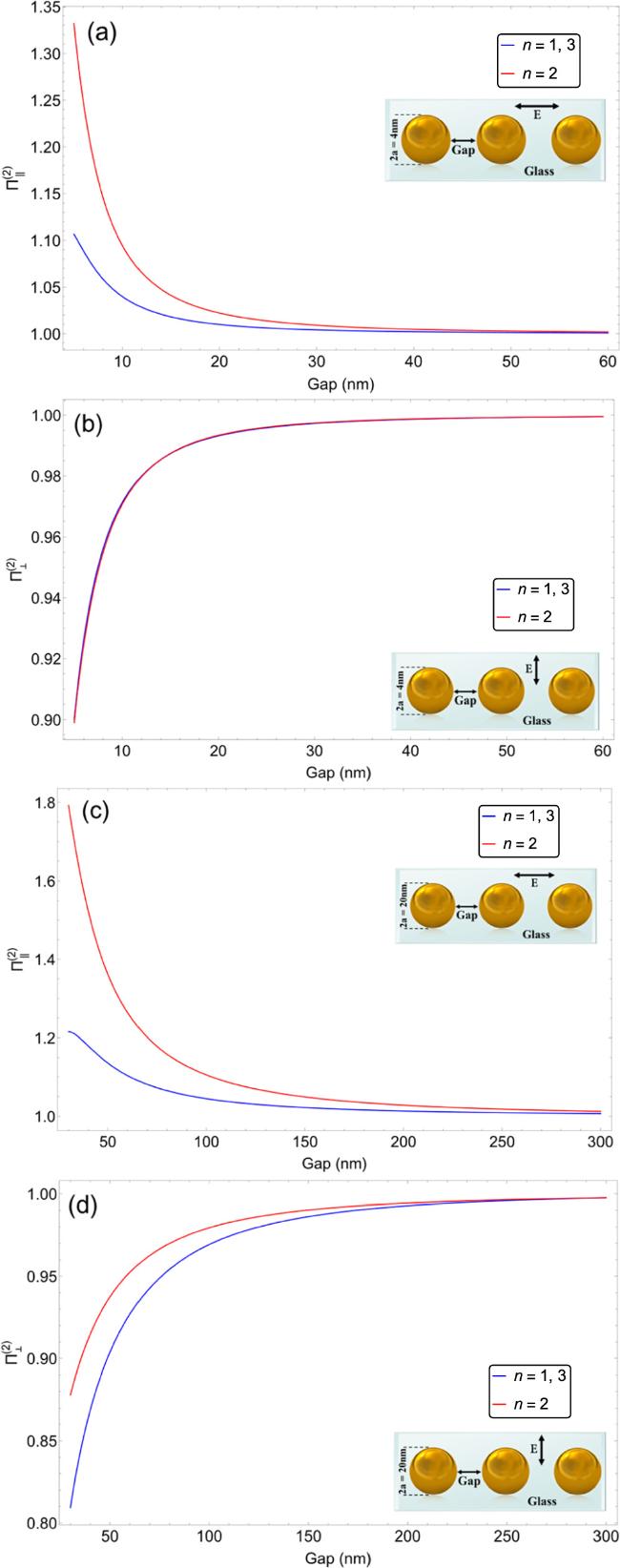
In order to show the influence of interparticle distance on the nonlinear dynamics of the trimer, in figures 4(a)–(d), for $a=2\,\rm{nm}$ and $a=10\,\rm{nm}$ and for both configurations, we have plotted the normalized SH peak power radiation of the NPs with respect to the gap distance of the NPs for both configurations. For all cases, when $g\gt 20a$, practically, interparticle interactions have no role in the dynamics of the system. Such a functionality of interparticle distance for the SH radiation of the planar array of Au NPs has been experimentally detected in [40].
Figure 4. The SHG efficiency with respect to the gap distance for (a, b) 2a = 4 nm and (c, d) 2a = 20 nm NP diameters and (a, c) parallel and (b, d) perpendicular laser beam polarizations. Here, n = 1, 2, 3 indicates the first, second and third NP, respectively. |
8. Conclusions
The SH generation of an MNP trimer was theoretically studied and analytical relationships were derived for the SH radiation power taking into account the dipole–dipole interaction of particles. The effect of laser beam polarization, the NPs size and their separation on the quality of SH generation was investigated. For the case when the laser beam electric field is parallel to the trimer axis, the interparticle interaction caused the increase in the SH radiation power and red-shift of plasmon peak, while for the perpendicular electric case the result was inverse, i.e. the reduction of the SH power and blue-shift of the plasmon peak. Additionally, it was observed that the effect of the interparticle dipole interaction on the middle NP is more intensive than other ones. Furthermore, the effect of the NPs gap on the SH radiation power was studied and it was found that after gap distance $g\gt 20a$, the NPs interaction has no important role on the trimer SHG power.