


1. Introduction
2. MC simulation results for the lattice φ4 model
Table 1. The values of ${\widetilde{\beta }}_{c}(L)$, χ/L7/4 and − (∂U/∂β)/L for λ = 0.1 and U = 1.1679229 ≈ U* depending on the lattice size L. |
| L | ${\widetilde{\beta }}_{c}$ | χ/L7/4 | − (∂U/∂β)/L |
|---|---|---|---|
| 6 | 0.6310451(76) | 1.92054(13) | 0.86991(19) |
| 8 | 0.6205904(55) | 1.70513(11) | 0.91937(19) |
| 12 | 0.6126206(35) | 1.494396(97) | 0.98891(23) |
| 16 | 0.6097694(27) | 1.394495(83) | 1.03316(23) |
| 24 | 0.6077895(17) | 1.302878(78) | 1.08511(27) |
| 32 | 0.6071420(14) | 1.261811(75) | 1.11200(29) |
| 48 | 0.60673002(87) | 1.226245(65) | 1.14005(32) |
| 64 | 0.60660154(68) | 1.210966(61) | 1.15320(34) |
| 96 | 0.60652379(44) | 1.198190(59) | 1.16602(37) |
| 128 | 0.60650059(31) | 1.192741(53) | 1.17128(36) |
| 192 | 0.60648656(21) | 1.188314(50) | 1.17676(38) |
| 256 | 0.60648299(17) | 1.186707(47) | 1.17978(37) |
| 384 | 0.60648037(11) | 1.185094(49) | 1.18112(38) |
| 512 | 0.606479833(90) | 1.184499(54) | 1.18115(45) |
| 768 | 0.606479199(84) | 1.183966(72) | 1.18249(67) |
| 1024 | 0.606479261(66) | 1.183828(71) | 1.18258(72) |
| 1536 | 0.606479163(42) | 1.183637(62) | 1.18270(72) |
| 2048 | 0.606479052(31) | 1.183539(72) | 1.18202(76) |
Table 2. The same quantities as in table 1 for λ = 0.1 and U = 2. |
| L | ${\widetilde{\beta }}_{c}$ | χ/L7/4 | − (∂U/∂β)/L |
|---|---|---|---|
| 6 | 0.5622957(89) | 0.500854(71) | 2.50489(62) |
| 8 | 0.5705578(64) | 0.446877(65) | 2.54550(65) |
| 12 | 0.5804632(43) | 0.394622(60) | 2.59107(77) |
| 16 | 0.5861528(33) | 0.370388(59) | 2.61472(77) |
| 24 | 0.5924095(22) | 0.349474(55) | 2.64609(86) |
| 32 | 0.5957579(16) | 0.341174(51) | 2.66479(96) |
| 48 | 0.5992428(11) | 0.335385(49) | 2.68905(95) |
| 64 | 0.60102839(66) | 0.333833(43) | 2.70895(94) |
| 96 | 0.60283621(49) | 0.333458(43) | 2.7284(10) |
| 128 | 0.60374599(36) | 0.333854(45) | 2.7382(11) |
| 192 | 0.60465782(23) | 0.334880(38) | 2.7563(11) |
| 256 | 0.60511400(17) | 0.335550(37) | 2.7625(11) |
| 384 | 0.60556994(12) | 0.336520(36) | 2.7729(11) |
| 512 | 0.60579760(11) | 0.336986(45) | 2.7772(15) |
| 768 | 0.606024909(96) | 0.337482(55) | 2.7827(20) |
| 1024 | 0.606138639(68) | 0.337825(56) | 2.7831(19) |
| 1536 | 0.606252317(45) | 0.338269(48) | 2.7885(18) |
| 2048 | 0.606308994(35) | 0.338425(52) | 2.7904(21) |
3. MC estimation of the correction-to-scaling exponent ω
3.1. Estimations from the susceptibility data
Table 3. The MC estimates of ω, obtained by fitting the susceptibility data in table 1 to the ansatz χ/L7/4 = A + BL−ω within $L\in [{L}_{{\rm{\min }}},2048]$. The quality of these fits is controlled by the χ2/d.o.f. and the goodness Q values in the last two columns. |
| ${L}_{{\rm{\min }}}$ | ω | χ2/d.o.f. | Q |
|---|---|---|---|
| 32 | 1.5124(27) | 7.92 | 7 · 10−12 |
| 48 | 1.5454(50) | 1.85 | 0.055 |
| 64 | 1.5567(78) | 1.61 | 0.115 |
| 96 | 1.577(16) | 1.52 | 0.154 |
| 128 | 1.546(24) | 1.34 | 0.237 |
Table 4. The MC estimates of ω, obtained by fitting the susceptibility data in table 2 to the ansatz χ/L7/4 = A + BL−ω + CL−1 within $L\in [{L}_{{\rm{\min }}},2048]$. The quality of these fits is controlled by the χ2/d.o.f. and the goodness Q values in the last two columns. |
| ${L}_{{\rm{\min }}}$ | ω | χ2/d.o.f. | Q |
|---|---|---|---|
| 24 | 1.269(14) | 3.98 | 1.9 · 10−5 |
| 32 | 1.333(20) | 2.37 | 0.011 |
| 48 | 1.431(40) | 1.61 | 0.117 |
| 64 | 1.540(69) | 1.24 | 0.276 |
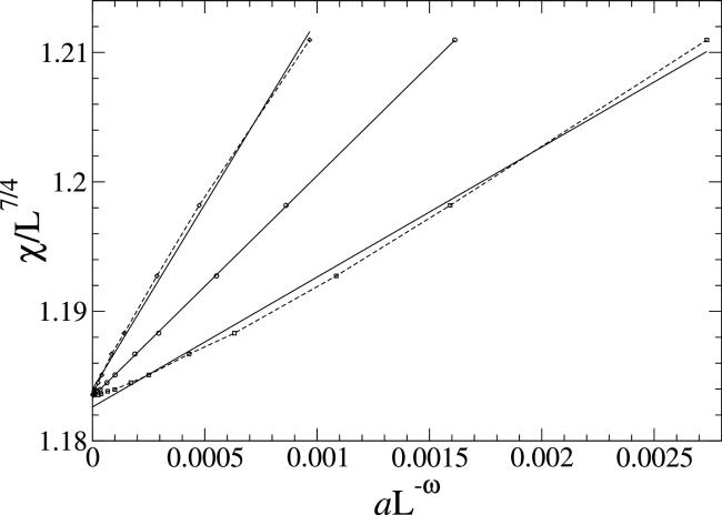
Figure 1. The χ/L7/4 versus aL−ω plots within L ∈ [64, 2048] for U = U* at a = 0.7, ω = 4/3 (squares); a = 1, ω = 1.546 (circles); and a = 1.4, ω = 7/4 (diamonds). The statistical errors of one σ are smaller than the symbol size. The linear fits are shown by straight lines. |
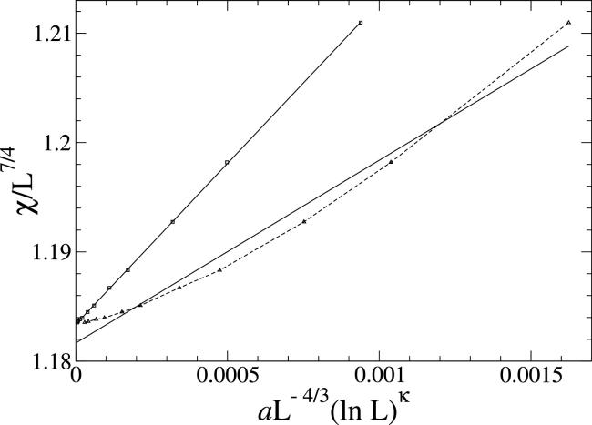
Figure 2. The χ/L7/4 versus $a{L}^{-4/3}{(\mathrm{ln}L)}^{\kappa }$ plots within L ∈ [64, 2048] for U = U* at a = 1, κ = − 1 (squares) and a = 0.1, κ = 1 (triangles). The statistical errors of one σ are smaller than the symbol size. The linear fits are shown by straight lines. |
3.2. Estimation from the ∂U/∂β data
Table 5. The MC estimates of ω, obtained by fitting the ∂U/∂β data in table 1 to the ansatz − (∂U/∂β)/L = A + BL−ω within $L\in [{L}_{{\rm{\min }}},2048]$. The quality of these fits is controlled by the χ2/d.o.f. and the goodness Q values in the last two columns. |
| ${L}_{{\rm{\min }}}$ | ω | χ2/d.o.f. | Q |
|---|---|---|---|
| 24 | 1.1747(95) | 5.96 | 8.3 · 10−10 |
| 32 | 1.246(15) | 2.41 | 0.0074 |
| 48 | 1.318(29) | 1.76 | 0.070 |
| 64 | 1.393(47) | 1.44 | 0.175 |
| 96 | 1.512(96) | 1.35 | 0.220 |
| 128 | 1.81(19) | 0.77 | 0.591 |
Table 6. The MC estimates of ω, obtained by fitting the ∂U/∂β data in table 1 to the ansatz − (∂U/∂β)/L = A + BL−ω + CL−2 within $L\in [{L}_{{\rm{\min }}},2048]$. The quality of these fits is controlled by the χ2/d.o.f. and the goodness Q values in the last two columns. |
| ${L}_{{\rm{\min }}}$ | ω | χ2/d.o.f. | Q |
|---|---|---|---|
| 8 | 1.2965(84) | 5.85 | 6.1 · 10−11 |
| 12 | 1.398(16) | 1.70 | 0.060 |
| 16 | 1.434(28) | 1.76 | 0.084 |
| 24 | 1.567(58) | 1.07 | 0.383 |
| 32 | 1.59(10) | 1.18 | 0.304 |
Table 7. The MC estimates of ω, obtained by fitting the ∂U/∂β data in table 2 to the ansatz − (∂U/∂β)/L = A + BL−ω within $L\in [{L}_{{\rm{\min }}},2048]$. The quality of these fits is controlled by the χ2/d.o.f. and the goodness Q values in the last two columns. |
| ${L}_{{\rm{\min }}}$ | ω | χ2/d.o.f. | Q |
|---|---|---|---|
| 16 | 0.4472(87) | 7.52 | 4.4 · 10−14 |
| 24 | 0.497(12) | 5.27 | 2.2 · 10−8 |
| 32 | 0.553(17) | 3.17 | 0.00045 |
| 48 | 0.629(26) | 1.61 | 0.105 |
| 64 | 0.621(33) | 1.80 | 0.072 |
| 96 | 0.715(54) | 1.32 | 0.234 |
| 128 | 0.850(85) | 0.69 | 0.657 |
Table 8. The MC estimates of ω, obtained by fitting the ∂U/∂β data in table 2 to the ansatz − (∂U/∂β)/L = A + BL−ω + CL−1 within $L\in [{L}_{{\rm{\min }}},2048]$. The quality of these fits is controlled by the χ2/d.o.f. and the goodness Q values in the last two columns. |
| ${L}_{{\rm{\min }}}$ | ω | χ2/d.o.f. | Q |
|---|---|---|---|
| 8 | 0.533(21) | 6.91 | 1.5 · 10−13 |
| 12 | 0.729(35) | 2.55 | 0.0022 |
| 16 | 0.819(49) | 2.11 | 0.017 |
| 24 | 1.039(93) | 1.37 | 0.186 |
| 32 | 1.08(14) | 1.51 | 0.139 |
| 48 | 0.92(21) | 1.61 | 0.117 |
| 64 | 1.61(44) | 1.05 | 0.392 |
3.3. Estimation from the pseudocritical couplings
Table 9. The MC estimates of ω, obtained by fitting the pseudocritical couplings in table 1 to the ansatz ${\widetilde{\beta }}_{c}(L)={\beta }_{c}+A\,{L}^{-1-\omega }$ within $L\in [{L}_{{\rm{\min }}},2048]$. The quality of these fits is controlled by the χ2/d.o.f. and the goodness Q values in the last two columns. |
| ${L}_{{\rm{\min }}}$ | ω | χ2/d.o.f. | Q |
|---|---|---|---|
| 32 | 1.4501(48) | 5.99 | 3.7 · 10−9 |
| 48 | 1.5019(91) | 1.28 | 0.243 |
| 64 | 1.509(14) | 1.38 | 0.198 |
| 96 | 1.531(29) | 1.47 | 0.172 |
| 128 | 1.511(46) | 1.67 | 0.124 |
Table 10. The χ2/d.o.f. and Q values for the fits of the pseudocritical couplings in table 1 to the ansatz ${\widetilde{\beta }}_{c}(L)={\beta }_{c}+A\,{L}^{-7/3}/\mathrm{ln}L$ within $L\in [{L}_{{\rm{\min }}},2048]$. |
| ${L}_{{\rm{\min }}}$ | χ2/d.o.f. | Q |
|---|---|---|
| 48 | 5.98 | 4 · 10−9 |
| 64 | 2.28 | 0.015 |
| 96 | 1.23 | 0.279 |
| 128 | 1.40 | 0.200 |
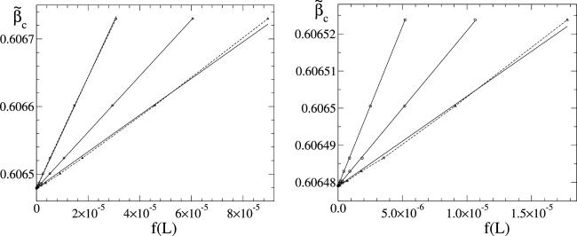
Figure 3. The ${\widetilde{\beta }}_{c}$ vs the f(L) plots at U = U* within L ∈ [48, 2048] (left) and L ∈ [96, 2048] (right) for f(L) = L−2.509 (circles), $f(L)={L}^{-7/3}/\mathrm{ln}L$ (squares) and f(L) = 0.75L−7/3 (triangles). The statistical errors of one σ are smaller than the symbol size in the left picture. These are about the same symbol size or smaller in the right picture. The linear fits are shown by solid straight lines. |
3.4. Summary of the MC estimations and comparison
4. The singularity of specific heat and the two-point correlation function
5. A renewed analysis by grouping of the Feynman diagrams
6. Summary and discussion
(i) In view of our best MC estimates (each from its own data set) valid for ∝ L−ω scaling of the non-analytical correction term, i.e., ω = 1.509(14), ω = 1.546(30), ω = 1.540(69), ω = 1.567(58) and ω = 1.61(44), the correction-to-scaling exponent ω is close to 1.5 if this scaling has, indeed, a pure power-law form. The most accurate estimate ω = 1.509(14) among these ones suggests that ω could be just 1.5, but we do not stress on this value, allowing for a slightly larger value as very probable. This concept is plausible from the point of view that the power-law scaling is the usual one. The only problem is that such values of ω are currently not confirmed by any exact result.
(ii) Looking for consistency with some exact result, we have found that ω is consistent with 4/3, provided that the ∝ L−ω scaling is modified by the logarithmic correction factor $1/\mathrm{ln}L$. The value 4/3 has been reported in [28] as the value of two coinciding correction-to-scaling exponents θ and $\theta ^{\prime} $, describing the fractal geometry of the critical Potts clusters in the case of the Ising model (q = 2) in two dimensions. We have considered the coincidence of these exponents as the reason for possible logarithmic correction. This conception seems to be very plausible from the point of view that it establishes the consistency with the exact exponent 4/3 found in [28]. However, we still have some concerns about its validity, since it is not rigorously clear whether or not the exponents θ and $\theta ^{\prime} $ are applicable to other quantities apart from those related to the fractal geometry of the critical Potts clusters. This is a relevant question from the point of view of the CFT discussed in [27], since the percolation problem of [28] is a nonunitary extension of the theory, and no correction exponent 4/3 has been found in the unitary φ4 theory, suggesting ω = 2. Nevertheless, we still consider options with ω ≠ 2 because the observed scaling of various quantities, e.g., ${\widetilde{\beta }}_{c}(L)$ at U = U* (accurately described by ω = 1.509(14) at κ = 0 in (
(iii) Considering logarithmic corrections, one more possibility has been revealed. Namely, the $\propto {L}^{-7/4}\mathrm{ln}L$ scaling with ω = 7/4 = 1.75 appears to be pretty well consistent with the data. This concept can be seen as plausible because the ω = 1.75 version is supported by the findings in [7], where this value of ω is considered to be exact. However, there are some concerns about the validity of this conception, too. The basic problem is the absence of any theoretical argument for the existence of the logarithmic correction in this case, noting that the data cannot be acceptably fit with ω = 1.75 without such a correction. A positive aspect, however, is that the logarithmic correction $\mathrm{ln}L$ is more usual than the $1/\mathrm{ln}L$ correction, and it really exists in many cases. A real support for ω = 1.75 comes from the ε-expansion in [7], yielding ω = 1.71(10), rather than from that suggested in [7]'s reference (our [27]), claiming ω = 2. The accuracy of the ε-expansion at ε = 2, however, is questionable.