


1. Introduction
Active matter is a non-equilibrium condensed system that encompasses various entities, including filaments driven by molecular motors [1, 2], bacteria propelled by flagella or cilia movement [3, 4], animal swarms [5], human crowds [6], and synthetic active particles driven by chemical reactions [7, 8], as shown in figure 1. The activity of these particles originates from self-propulsion and generates highly correlated cluster motions. Active matter does not satisfy equilibrium conditions and the transition between microstates breaks the time-reversal symmetry. Another significant feature of active matter is the presence of non-negligible random fluctuations in the movement of individual active units [9] caused by environmental factors or internal fluctuations. For instance, actin filaments have biochemical processes that generate forces or motion in a non-deterministic way. The interplay of driving forces with intrinsic noise can give rise to rich phase behaviors not observed in equilibrium systems, such as the spontaneous formation of flocking motion, as shown in figure 1(c).
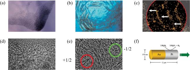
Figure 1. (a) A flock of birds responding to predators by flying in parallel. (b) A school of fish spontaneously forming a vortex-like columnar structure. (c) Polar order in actin filaments driven by molecular motors. (d) Active turbulence in Bacillus subtilis. (e) A monolayer of vibrating rods forming the nematic order with topological defects, where the red circle indicates a mobile + 1/2 defect and the green circle indicates an immobile −1/2 defect. (f) Random walk of gold-platinum rods driven by hydrogen peroxide. Images adopted from [1, 5, 8, 10, 11]. |
Wet active matter involves active particles that interact with a surrounding fluid. The presence of fluid leads to hydrodynamic interactions, which significantly influence the collective behavior of particles. By contrast, the interactions in dry active matter are typically limited to direct mechanical contacts, friction, or other non-hydrodynamic forces. Dry active particles can be divided into two categories: aligning and non-aligning particles. Aligning active matter refers to active systems composed of self-propelled particles that tend to align their directions of motion with their neighbors due to the elongated body or social cooperativity, whereas non-aligning active matter lacks this tendency. Distinguished by the interactions and intrinsic geometrical properties, there are six types of dry aligning active matter (DAAM): (1) polar active particles: particles aligned along their moving directions due to orientational forces; (2) self-propelled rods: elongated rods with forces aligning their long axes parallel to each other and moving along the direction of their heads; (3) active nematics: elongated units with head–tail symmetry and characterized by chaotic flows without directed motion of individual units, which move along their long axis due to the shape and propulsion mechanism; (4)–(6) chiral counterparts of the above three types of aligning active particles. The cartoons of these six kinds of DAAM are illustrated in figure 2. Active materials with other types of interactions or combination of features, such as chemotactic [12], dipolar [13], non-reciprocal [14] interactions, and self-propelled particles with velocity reversals and polar alignment [15], are beyond the scope of this review.
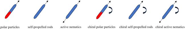
Figure 2. The cartoons of aligning active particles. Aligning active particles are generally self-propelled along their long axis, where black arrows indicate the velocity direction and right curved arrows indicate the clockwise chirality. Polar particles have head–tail asymmetry and orientational forces (polar alignment). Active nematics have head–tail symmetry and nematic forces, while self-propelled rods lack this symmetry but still experience nematic forces. Chiral aligning active particles have an intrinsic asymmetry that enables them to move in a curved or helical trajectory and exhibit left-handed or right-handed chirality. |
These six types of DAAM have corresponding experimental systems. Migrating animal herds [5, 16], migrating cell layers [17], vibrated asymmetric granular particles [18], and swimming bacillus subtilis bacteria [19] are some examples of polar particles. Many systems fall in the category of self-propelled rods, including DNAs with diffusiophoretic motion [20], and elongated myxobacteria driven by flagella characterized by rippling, streaming, and aggregation when they are starving [21, 22]. Examples of active nematics are elongated amoeboid [23, 24] cells, which exhibit non-directed motion. Vertically vibrated granular rods exhibit vortical pattern with certain number of rods, vibration amplitude, and frequency [25]. Active Filaments, such as microtubules or actin filaments, are driven by molecular motors like kinesin, dynein, or myosin that consume ATPs [26]. The activity of these motor proteins generates stress and flows. Chiral active particles typically exhibit chiral shapes [27], anisotropic [28] or non-reciprocal [29] interactions, or hydrodynamic interactions with walls or interfaces [30], thereby breaking the mirror symmetry. Examples of chiral polar particles include right-hand E. coli [31], sperm cells [32], magnetotatic bacteria in a rotating field [33], curved polymer [34], and synthetic swimmers with an L-shape [35]. Vibrioid or helical bacteria are typical chiral self-propelled rods [36], such as Caulobacter crescentus of crescent shape and Helicobacter pylori of helix form [37, 38]. Nematic cell monolayers [39], are typical chiral active nematics.
The collective behavior of active matter varies across different density limits. In the low-density regime or dilute limit, interactions between particles are infrequent, and the behavior of individual particles is more prominent [9]. In the intermediate-density regime, interactions between particles become more significant, leading to a variety of emergent collective behaviors, such as flocking, clustering, and pattern formation [5]. In the high-density limit, repulsive forces play an important role, leading to the formation of crystalline [40], jamming, and glassy phases [41]. At high densities, with increasing strength of the orientational force, polar particles undergo a reentrant glass transition towards a polarized amorphous solid [42].
Investigating phase transitions in DAAM helps understanding how phase transitions occur, what governs their behavior, and what are the underlying principles that apply across different types of active systems. DAAM may exhibit novel phase behaviors without direct analogues in corresponding non-active systems, such as flocking [5], active turbulence [43], and motility-induced phase separation which can arise solely from motility and excluded-volume effects [44]. As a result, studying these phenomena broadens our understanding of phases and phase transitions. The phase transitions of DAAM have attracted great interest since the development of the Vicsek model [45], a pioneer work in the study of self-organizing phenomena connecting microscopic interactions with macroscopic phase behaviors. There is an ongoing debate about whether the phase transition in the Vicsek model is continuous or discontinuous [46–48].
This review is focused on phase transitions of DAAM, which has been intensively studied in two-dimension. There are mainly three types of phase transitions for DAAM: continuous, discontinuous, and topological. The continuous phase transitions are characterized by a continuous change in the order parameter and critical phenomena, the discontinuous phase transitions are marked by a sudden change in the order parameter, and the topological phase transitions are associated with changes in the topological invariants that cannot be described by order parameters. We will emphasize general characteristics of phase transitions and the determination of phase transition points. The characteristics of equilibrium and dynamic phase transitions are also described.
2. Methods
2.1. Simulation models and order parameters
The Vicsek model is foundational in simulating active matter, showing how simple local rules can result in complex collective behaviors, such as the synchronized flight of bird flocks. The Vicsek model (VM) [45], mimics dry polar active matter in the dilute system, where repulsive interactions are ignored. Simulations utilizing the Vicsek model usually have the periodic boundary conditions applied. At each time step, N particles update their velocities simultaneously according to the average velocity direction of neighboring particles subject to a random noise as
$\begin{eqnarray}{{\boldsymbol{r}}}_{i}\left(t+{\rm{\Delta }}t\right)={{\boldsymbol{r}}}_{i}\left(t\right)+{v}_{0}\hat{{\boldsymbol{n}}}\left({\theta }_{i}\left(t\right)\right){\rm{\Delta }}t,\end{eqnarray}$
$\begin{eqnarray}{\theta }_{i}={\rm{\Theta }}\left({{\boldsymbol{v}}}_{i}+\displaystyle \displaystyle \sum _{\left|{{\boldsymbol{r}}}_{i}-{{\boldsymbol{r}}}_{j}\right|\lt R}{{\boldsymbol{v}}}_{j}\right)+{\zeta }_{i},\end{eqnarray}$
where ${{\boldsymbol{r}}}_{i}$ is the position of particle i, ${v}_{0}$ is the magnitude of the self-propulsion velocity, $\hat{{\boldsymbol{n}}}\left({\theta }_{i}\right)$ is the normal vector of the orientation angle ${\theta }_{i}$, ${\rm{\Delta }}t$ is the time step, ${\rm{\Theta }}\left({\boldsymbol{v}}\right)$ is the direction of vector ${\boldsymbol{v}}$, $R$ is the radius of polar interaction, ${\zeta }_{i}$ is a uniform white noise in the range of $\left[-\eta /2,\,\eta /2\right]$, and $\eta $ is the noise strength. Other models for dry polar active particles are usually modified on top of the Vicsek model, and thus can be viewed as Vicsek-like models (VLM).The motion of a DAAM may alternatively be described by the overdamped Langevin dynamics [48, 49]
$\begin{eqnarray}{{\boldsymbol{v}}}_{i}=A{v}_{0}{\boldsymbol{n}}\left({\theta }_{i}\right)+\displaystyle \frac{1}{{\gamma }_{0}}{{\boldsymbol{F}}}_{i}^{{\rm{r}}},\end{eqnarray}$
$\begin{eqnarray}{\dot{\theta }}_{i}={\omega }_{i}+\displaystyle \frac{K}{{n}_{i}}\displaystyle \displaystyle \sum _{\left|{{\boldsymbol{r}}}_{i}-{{\boldsymbol{r}}}_{j}\right|\lt R}\sin \left[m\left({\theta }_{j}-{\theta }_{i}\right)\right]+\sqrt{2{D}_{{\rm{r}}}}{\xi }_{i},\end{eqnarray}$
where A represents the sign of the self-propelled velocity, ${\gamma }_{0}$ is the damping coefficient, ${{\boldsymbol{F}}}_{i}^{{\rm{r}}}$ is the short-ranged repulsive force, ${\omega }_{i}$ is the intrinsic rotational rate drawn from a zero-mean distribution whose root-mean-square is ${\omega }_{0}$, $K$ is the strength of the alignment force, ${n}_{i}$ is the number of neighbors of particle i, m is an integer, ${D}_{{\rm{r}}}$ is the rotational diffusion constant, and ${\xi }_{i}$ is the Gaussian white noise [50] satisfying $\begin{eqnarray}\left\langle {\xi }_{i}\left(t\right)\right\rangle =0;\left\langle {\xi }_{i}\left(t\right){\xi }_{j}\left(t^{\prime} \right)\right\rangle ={\delta }_{i,j}\delta \left(t-t^{\prime} \right).\end{eqnarray}$
In the above model, alignment is polar for m = 1 and nematic for m = 2. Both self-propelled particles and active nematics exhibit nematic alignment. For polar and self-propelled particles, A = 1. Active nematics additionally exhibit velocity reversals with $A=\pm 1$, namely, their velocities change their signs A at a certain rate $a$. Chiral active particles have an intrinsic non-zero rotational rate related to the phenomenon that a group of coupled oscillators in the Kuramoto model [51, 52] spontaneously synchronizes to a common frequency. There are four dimensionless parameters: the packing fraction ${\rho }_{{\rm{r}}}=\frac{N\pi {R}_{{\rm{r}}}^{2}}{{L}^{2}}$ which compares the volume occupied by the particles with the volume of the system, the rotational Péclet number ${{\rm{Pe}}}_{{\rm{r}}}=\frac{{v}_{0}}{{D}_{{\rm{r}}}{R}_{{\rm{r}}}}=\frac{{l}_{{\rm{p}}}}{{R}_{{\rm{r}}}}$ which quantifies the effective self-propulsion strength, the effective alignment intensity $g=\frac{K}{{D}_{{\rm{r}}}}$ which compares the aligning tendency of velocity direction with the tendency for random reorientation, and the effective rotational rate ${\rm{\Omega }}=\frac{{\omega }_{0}}{{D}_{{\rm{r}}}}$ which compares the strength of deterministic and stochastic contributions to the orientation angle, where ${R}_{{\rm{r}}}$ is the characteristic length of the repulsive force and ${l}_{{\rm{p}}}$ is the persistence length.The average velocity $\varphi $ serves as a measure of the degree of polar order parameter
$\begin{eqnarray}\varphi =\displaystyle \frac{1}{N{v}_{0}}\left|\displaystyle \sum _{i=1}^{N}{{\boldsymbol{v}}}_{i}\right|,\end{eqnarray}$
where N is the number of particles. The polar order parameter $\phi =\left\langle \varphi \right\rangle $, where $\left\langle \right\rangle $ denotes ensemble average.The nematic order parameter for self-propelled rods and active nematics is defined as
$\begin{eqnarray}S=\left\langle \displaystyle \frac{3{\cos }^{2}{\theta }_{n}-1}{2}\right\rangle ,\end{eqnarray}$
where ${\theta }_{n}$ is the orientational angle of the long axis of a liquid crystal molecule. S usually varies between 0 and 1. S = 0 signifies the absence of nematic order, whereas S = 1 indicates perfect alignment of the system.2.2. Hydrodynamic theories
The continuum models use hydrodynamic theories to translate the microscopic interactions of individual active particles into macroscopic fields like density, velocity, and orientation by coarse graining and some assumptions. This approach enables the study of large-scale behaviors and patterns of active matter.
There are several ways to derive hydrodynamic equations [53]. One approach involves augmenting the Navier–Stokes equations with terms permitted by symmetries, using phenomenological coefficients, as seen in models like the Toner–Tu model [54, 55]. Alternatively, by employing the molecular chaos hypothesis, the Boltzmann–Ginzburg–Landau and Fokker–Planck/Smoluchowski approaches describe the temporal evolution of the one-body probability density function [56]. This is achieved by coarse-graining a microscopic model and truncating Fourier series expansions. The Boltzmann equation accounts for free evolution, self-diffusion, and collisions at low densities, while the Fokker–Planck equation incorporates advection, angular diffusion, noise, and mean-field interactions. The Enskog-type equation extends the Boltzmann equation to include multi-body collisions [57]. Through stability analysis, one can perturb the steady-state solution slightly to determine its robustness and stability. The reference frame for dry active matter is defined by the surface or medium in which it is situated, and thus it does not adhere to Galilean invariance.
John Toner and Yuhai Tu [55], utilized a phenomenological approach to derive the following continuum model for dry polar active matter:
$\begin{eqnarray}\begin{array}{lll}{\partial }_{t}{\boldsymbol{v}}+{\lambda }_{1}\left({\boldsymbol{v}}\cdot {\rm{\nabla }}\right){\boldsymbol{v}}+{\lambda }_{2}\left({\rm{\nabla }}\cdot {\boldsymbol{v}}\right){\boldsymbol{v}}+{\lambda }_{3}{\rm{\nabla }}\left(| {\boldsymbol{v}}{| }^{2}\right) & = & \alpha {\boldsymbol{v}}-{\beta }_{0}| {\boldsymbol{v}}{| }^{2}{\boldsymbol{v}}\\ & & \,-\,{\rm{\nabla }}P+{D}_{1}{\rm{\nabla }}\left({\rm{\nabla }}\cdot {\boldsymbol{v}}\right)\\ & & \,+\,{D}_{2}{{\rm{\nabla }}}^{2}{\boldsymbol{v}}+{D}_{3}{({\boldsymbol{v}}\cdot {\rm{\nabla }})}^{2}{\boldsymbol{v}}+{\boldsymbol{f}}{\boldsymbol{,}}\end{array}\end{eqnarray}$
$\begin{eqnarray}P=\displaystyle \sum _{n=1}^{\infty }{\sigma }_{n}{\left(\rho -{\rho }_{0}\right)}^{n},\end{eqnarray}$
$\begin{eqnarray}\left\langle {f}_{i}\left(t,{\boldsymbol{r}}\right){f}_{j}\left({t}^{{\rm{{\prime} }}},{{\boldsymbol{r}}}^{{\rm{{\prime} }}}\right)\right\rangle ={\rm{\Delta }}{\delta }_{{ij}}{\delta }^{d}\left({\boldsymbol{r}}-{{\boldsymbol{r}}}^{{\rm{{\prime} }}}\right)\delta \left(t-{t}^{{\rm{{\prime} }}}\right),\end{eqnarray}$
where $\rho $ is the density field, ${\rho }_{0}=\frac{N}{{L}^{2}}$ is the average density, $P$ is the pressure field, ${\boldsymbol{f}}$ is the Gaussian white noise, ${\rm{\Delta }}$ is a constant, and d is the spatial dimension. In order to satisfy the symmetry, ${\lambda }_{i}$, $\alpha $, ${\beta }_{0}$, ${D}_{i}$, and ${\sigma }_{n}$ are functions of $| {\boldsymbol{v}}{| }^{2}$ and $\rho $, where $i=1,2,3$. The Toner–Tu model satisfies the continuity equation derived from the conservation of particle number $\begin{eqnarray}\displaystyle \frac{\partial \rho }{\partial t}+{\rm{\nabla }}\cdot \left({\boldsymbol{v}}\rho \right)=0.\end{eqnarray}$
The continuum models for dry polar active matter can also be derived from the Boltzmann–Ginzburg–Landau [57–59] or Fokker–Planck approaches [56, 60, 61].For self-propelled rods, by deriving Boltzmann equations [62–64] or Fokker–Planck equations [65, 66], one can expand the one-body probability density function $f\left({\boldsymbol{r}},\theta ,t\right)\,=\frac{1}{2\pi }\displaystyle \sum _{k=-\infty }^{\infty }{f}_{k}\left({\boldsymbol{r}},t\right){{\rm{e}}}^{-{\rm{i}}k\theta }$ to get the polar field ${\boldsymbol{P}}=\frac{1}{\rho }\left(\begin{array}{c}\mathrm{Re}{f}_{1}\\ \rm{Im}{f}_{1}\end{array}\right)$ and the nematic order parameter tensor ${\boldsymbol{Q}}=\frac{1}{2\rho }\left(\begin{array}{cc}\mathrm{Re}{f}_{2} & \rm{Im}{f}_{2}\\ \rm{Im}{f}_{2} & -\mathrm{Re}{f}_{2}\end{array}\right)$. Then, one can write down the following closed equations:
$\begin{eqnarray}\begin{array}{lll}{\partial }_{t}{f}_{1} & = & -\displaystyle \frac{1}{2}\left({\rm{\nabla }}\rho +{{\rm{\nabla }}}^{\ast }{f}_{2}\right)+\displaystyle \frac{{\gamma }_{1}}{2}{f}_{2}^{\ast }{\rm{\nabla }}{f}_{2}\\ & & -\,\left(\alpha -{\beta }_{0}{\left|{f}_{2}\right|}^{2}\right){f}_{1}+\varsigma {f}_{1}^{\ast }{f}_{2},\end{array}\end{eqnarray}$
$\begin{eqnarray}\begin{array}{lll}{\partial }_{t}{f}_{2} & = & -\displaystyle \frac{1}{2}{\rm{\nabla }}{f}_{1}+\displaystyle \frac{o}{4}{{\rm{\nabla }}}^{2}{f}_{2}-\displaystyle \frac{{\kappa }_{0}}{2}{f}_{1}^{\ast }{\rm{\nabla }}{f}_{2}-\displaystyle \frac{{\chi }_{0}}{2}{{\rm{\nabla }}}^{\ast }\left({f}_{1}{f}_{2}\right)\\ & & +\,\left({\mu }_{0}-\xi {\left|{f}_{2}\right|}^{2}\right){f}_{2}+\omega {f}_{1}^{2}+\tau {\left|{f}_{1}\right|}^{2}{f}_{2},\end{array}\end{eqnarray}$
where all coefficients depend only on the noise strength $\eta $ and the density field $\rho $. The gradient ${\rm{\nabla }}={\partial }_{x}+{\rm{i}}{\partial }_{y}$ is a complex operator.For active nematics, the continuum model can also be derived by the Toner–Tu framework [67, 68], the Boltzmann–Ginzburg–Landau approach [69], and the Fokker–Planck approach [70]. For chiral polar particles, the Boltzmann equations [71] and the Fokker–Planck [53] equations are employed. For chiral self-propelled rods, the Fokker–Planck equations are employed [72]. For chiral active nematics, the nematohydrodynamic equations are a set of continuum equations that describe the orientational order of elongated particles, accounting for both their chirality and active nature [73].
3. Continuous phase transitions
For the continuous thermodynamic phase transition in equilibrium, the second or higher derivative of the free energy diverges at the critical point, the order parameter is continuous around this point, and there exist critical exponents. Some critical exponents can be estimated via finite-size scaling [74]. The scaling laws reveal that these critical exponents are universal, depending only on the dimensionality and symmetry of the system rather than its microscopic details. At the critical temperature, the Binder cumulant of order parameter for different system sizes intersects at the same point [75]. The correlation length and susceptibility diverge when approaching the critical point, exhibiting a power-law behavior that signifies large responses to small perturbations [76]. The renormalization group theory aids in determining the critical points, critical exponents, and universal classes of the Ising model [77, 78]. According to the Landau–de Genne theory [79], when the external field is very strong, the thermotropic isotropic-nematic phase transition of liquid crystal is continuous.
The Mermin–Wagner theorem states that two-dimensional systems with continuous rotational symmetry have no long-range order at finite temperatures [80]. In the context of animals with a specific field of view, the critical noise tends to 0 when the viewing angle for VLM is less than $\pi $ [81], which is in accordance with the Mermin–Wagner theorem. The Berezinskii–Kosterlitz–Thouless (BKT) theory shows that such systems can exhibit quasi-long-range order, where the order-parameter correlation function decays according to a power law [82]. In the limit of speed ${v}_{0}$ approaching 0, the VM is similar to the XY model [83]. However, when the noise is weak, all polar active particles align their flights in parallel, indicating a continuous symmetry breaking and resulting in a global polar order. At high noise intensities, particle velocity directions are heavily perturbed by random fluctuations, leading to the absence of a global polar order. As the noise strength increases, the transition from the polar ordered phase to the disordered phase occurs. At low velocities $\left({v}_{0}\leqslant 0.1\right)$, due to the absence of a minimum in the Binder cumulant near the phase transition point and the fact that the distribution of the order parameter exhibits only a single peak, Vicsek et al suggested that the Vicsek model exhibits a continuous phase transition [84]. However, this conclusion may be unreliable due to the limitations imposed by the finite system size and the restricted simulation time [85].
With increasing density, thermal hard rods of length $l$ undergo a continuous isotropic-nematic transition (INT) at a density ${\rho }_{N}=3/\left(\pi {l}^{2}\right)$ [86]. For self-propelled rods, the density of INT [66, 87, 88] is
$\begin{eqnarray}{\rho }_{{\rm{IN}}}=\displaystyle \frac{{\rho }_{N}}{1+\displaystyle \frac{{v}_{0}^{2}}{5{k}_{{\rm{B}}}T}}.\end{eqnarray}$
In active systems, an ordered state emerges at lower densities due to additional momentum transfer from self-propulsion.3.1. Continuity of the order parameter
In the noise-induced phase transition, the polar order parameter is continuous for the VM, as depicted in figure 3(a), the momentum-conserving VLM [89], and the metric-free(topological) models [90–92], with the neighboring particles determined by the Voronoi [90] or k-nearest [91, 93, 94] algorithm. In the metric-free model whose interactions are no longer based on the distance, stability analysis of the hydrodynamic description suggests that a density-independent collision rate per particle prevents the formation of the band phase [95] characterizing continuous phase transitions. These topological models are crucial in studying animal groups [96–99] or pedestrians [100]. Besides, increasing the density reveals a continuous change of the order parameter with a weak orientational force in the dense polar system [42].
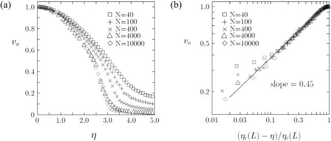
Figure 3. Features of continuous phase transitions close to the phase transition point in the Vicsek model at low velocities, including: (a) Continuous behavior of the order parameter ${v}_{a}=\left\langle \varphi \right\rangle $; (b) scaling of the order parameter. Images adopted from [45]. |
The nematic order parameter of active nematics S becomes continuous as the density of filaments or motors increases in INT [101]. Specifically, through simulations and using the Smoluchowski equation, Kraikivski et al [101] have determined that the transition point satisfies $S=0.2$. In experiments with confined granular rods, the nematic order parameter remains continuous during the isotropic-nematic transition, achieved by varying the length-to-diameter ratio [102].
3.2. Critical exponents and scaling relation
As the system size $L\to \infty $, the scaling of the polar order parameter for the VM is
$\begin{eqnarray}\phi \unicode{x0007E}\left\{\begin{array}{ll}{\varepsilon }^{\beta } & {\rm{for}}\eta \lt {\eta }_{c}({\rho }_{0},L)\\ 0 & {\rm{for}}\eta \gt {\eta }_{c}({\rho }_{0},L)\end{array}\right.,\end{eqnarray}$
where $\varepsilon =\frac{{\eta }_{c}\left({\rho }_{0},L\right)-\eta }{{\eta }_{c}\left({\rho }_{0},L\right)}$ is the reduced noise, ${\eta }_{c}$ is the critical noise intensity, and $\beta $ is the critical exponent. $\beta =0.45$ for the VM [45], different from the mean-field value of $1/2$ [103], as shown in figure 3(b). The scaling of the fluctuation is $\begin{eqnarray}X=\left(\left\langle {\varphi }^{2}\right\rangle -{\left\langle \varphi \right\rangle }^{2}\right){L}^{2}\sim {\left|\varepsilon \right|}^{-\gamma },\end{eqnarray}$
where $\gamma \approx 2$ for the VM.Finite-size scaling is a useful tool for studying out-of-equilibrium phase transitions even in the absence of a rigorous statistical theory [104, 105]. The finite-size scaling ansatz [106] is
$\begin{eqnarray}\phi \left(\varepsilon ,L\right)={L}^{-\beta /\nu }\tilde{\phi }\left(\varepsilon {L}^{1/\nu }\right),\end{eqnarray}$
$\begin{eqnarray}X\left(\varepsilon ,L\right)={L}^{\gamma /\nu }\tilde{X}\left(\varepsilon {L}^{1/\nu }\right),\end{eqnarray}$
where $v$ is the critical exponent of correlation length, and $\tilde{\phi }$ or $\tilde{X}$ is the scaling function. Considering the scaling relations $\left\langle {\varphi }^{n}\right\rangle \propto {L}^{-n\beta /\nu }$ at the phase transition point ${\eta }_{c}\left({\rho }_{0},\infty \right)$, the Binder cumulant of the order parameter $G=1\,-\left\langle {\varphi }^{4}\right\rangle /\left(3{\left\langle {\varphi }^{2}\right\rangle }^{2}\right)$ for different system sizes intersects at a universal point of VM [107] and VLM [90], which determines the critical point.With the VM, Vicsek et al [108] studied the susceptibility $\chi \left(\eta \right)=\mathop{\mathrm{lim}}\limits_{h\to 0}\left(\phi (\eta ,h)-\phi (\eta ,h=0)\right)/h$ with respect to the external field. The equation of velocity direction is replaced by
$\begin{eqnarray}{\theta }_{i}={\rm{\Theta }}\left({{\boldsymbol{v}}}_{i}+\displaystyle \displaystyle \sum _{\left|{{\boldsymbol{r}}}_{i}-{{\boldsymbol{r}}}_{j}\right|\lt R}{{\boldsymbol{v}}}_{j}+h{\boldsymbol{e}}\right)+{\zeta }_{i},\end{eqnarray}$
where ${\boldsymbol{e}}$ is the arbitrary unit vector and h is the strength of the perturbation. They obtained the relation $\begin{eqnarray}\phi \left(\eta ,h\right)=\chi \left(\eta \right){h}^{\displaystyle \frac{1}{\delta }};\chi \left(\eta \right)={\left|\varepsilon \right|}^{-\gamma ^{\prime} },\end{eqnarray}$
where the critical exponent $\delta =1.1$ and critical exponent $\begin{eqnarray}\left(\gamma ^{\prime} \right)\approx \left\{\begin{array}{ll}1 & {\rm{for}}\,\eta \lt {\eta }_{c}({\rho }_{0},L)\\ 4 & {\rm{for}}\,\eta \gt {\eta }_{c}({\rho }_{0},L)\end{array}\right..\end{eqnarray}$
These critical exponents remain unchanged even when a repulsive interaction is introduced [109], but the critical exponents differ between the approach using the vectorial noise with a forward update rule and the method employing the angular noise with a backward update rule, indicating that they belong to different universality classes.There is a hyperscaling relation connecting the VM [107] and the VLM [90, 109]:
$\begin{eqnarray}\gamma +2\beta =vd,\end{eqnarray}$
where d denotes the spatial dimension. Fisher's scaling law is given by [110] $\begin{eqnarray}\gamma =v\left(2-\kappa \right),\end{eqnarray}$
where $\kappa $ is the critical exponent that characterizes the decay of the correlation function at the critical point.4. Discontinuous phase transitions
For discontinuous phase transitions in equilibrium, at the phase transition point, the first derivative of the free energy diverges, and the order parameter that characterizes symmetry breaking undergoes an abrupt change. At the transition temperature or pressure, the two phases (e.g. solid and liquid) coexist in equilibrium. The presence of energy barrier during the transition leads to hysteresis. In the ordered phase, the Binder cumulant of the order parameter approaches 2/3, while in the disordered phase with a continuous rotational symmetry, it takes a value around 1/3. Near the phase transition point, the Binder cumulant of the order parameter reaches a minimal value below zero [111]. In the nematic phase, molecules of the liquid crystal exhibit long-range nematic order. As temperature increases, there occurs a weak discontinuous phase transition from the nematic phase to a disordered isotropic phase with a slight latent entropy at the transition [112].
At a high speed ${v}_{0}\geqslant 0.3$, Chaté et al [113], suggest that the VM undergoes a discontinuous phase transition, as the order parameter is discontinuous near the phase transition point, the Binder cumulant G has a minimum less than zero, and the distribution of the order parameter exhibits two peaks. However, this conclusion may be unreliable due to the interplay between the anisotropic diffusion and the periodic boundary conditions [84]. Simulations adopting the vectorial noise in the VM exhibit first-order phase transitions with both backward and forward updates [114]. If the alignment range is small, the phase transition exhibits discontinuous behavior characterized by cluster formation. In contrast, with a large alignment range, the phase transition becomes continuous [115], akin to the one-dimensional model [116]. Chen et al [47] employed relative local density and velocity to construct microstates forming an ensemble matrix and investigated the finite-size effects of singular values as the order parameters. Their findings revealed that the velocity-based order parameter undergoes a continuous transition, while the density-based order parameter exhibits a discontinuous transition.
4.1. Discontinuity of the order parameter
As shown in figure 4(a), when the system size L is large enough, there is a discontinuous change of the order parameter at the phase transition point, in the VM or the VLM with vectorial noise, which can be induced by shear stress [117]. According to the geometric interpretation of information, the curvature of internal energy diverges at the phase transition point in the VLM [118]. With increasing alignment strength, the configurational entropy and the rates for the change of work and internal energy decrease. Besides, increasing the density reveals a discontinuous change for the order parameter with a strong alignment force in the dense polar system [42].
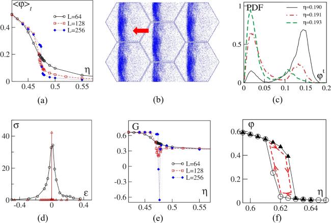
Figure 4. Characteristics of discontinuous phase transitions near the phase transition point in the VM and VLM at high velocities. (a) The order parameter is discontinuous $\left(\rho =2,{v}_{0}=0.5\right)$; (b) High-density band structures coexist with low-density disordered gas for a hexagonal simulation cell, visualized by points representing particle positions, and the red arrow indicates band-structure movement direction $\left(\rho =2/\sqrt{3},{v}_{0}=10,L=128/\sqrt{3}\right)$; (c) The reduced average velocity exhibits a bimodal distribution, indicative of spontaneous transitions between band and disordered phases $\left(\rho =0.125,{v}_{0}=0.5,L=512\right)$; (d) The variance $\sigma ={L}^{2}\left(\left\langle {\varphi }^{2}\right\rangle -{\left\langle \varphi \right\rangle }^{2}\right)$ exhibits an abrupt peak $\left(\varepsilon =\left({\eta }_{{\rm{c}}}-\eta \right)/{\eta }_{{\rm{c}}},\rho =2,{v}_{0}=0.5,L=64\right)$; (e) The Binder cumulant G exhibits minima below 0 $\left(\rho =2,{v}_{0}=0.5\right)$; (f) A hysteresis phenomenon is observed, characterized by parameter changes over time, illustrated by red arrows $\left(\rho =0.5,{v}_{0}=0.5,L=32\right)$. The symbol $\eta $ used in the pictures is $2\pi $ times the previously defined symbol $\eta $. The density $\rho =N/{L}^{d}$. Figures 4(a)–(e) illustrate the VM, while figure 4(f) shows the VLM in three dimensions with a vectorial noise. Images adopted from [84, 85, 113]. |
4.2. Phase coexistence
Phase coexistence, a characteristic of discontinuous phase transitions, can be categorized into spatial coexistence and temporal coexistence. For spatial phase coexistence of the VM, a disordered gas coexists with band structures [85], with a well-defined width and a peak in the structure factor at low wave numbers, as shown in figure 4(b). This phenomenon persists even in the fore-and-aft asymmetric VLM [119], the VLM with complex nonlinear noise [120], or the VLM with limited-vision cones [121]. The superdiffusion impedes the formation of large band domains in this phase, contrasting with normal fluctuations observed in the active Ising model. The band phase in the VM can be elucidated using stochastic scalar and vectorial partial differential equations [122], whereas full phase separation in the active Ising model can be described by similar frameworks [123]. For large system sizes, the cross-sea phase appears in the VM as a superposition of two waves intersecting at a characteristic crossing angle [124]. The wavelength of the cross-sea pattern is approximately twice that of the band pattern. The band phase, supported by the Enskog-like kinetic theory [125] and the phenomenological approach [126], remains stable at noise intensities higher than those of the cross-sea phase, as identified using convolutional neural networks [127].
For phase coexistence over time, the system in the VM switches between high-speed band phases and low-speed disordered phases, leading to a bimodal distribution of the reduced average velocity, as shown in figure 4(c). Due to the sudden increase in the fourth moment of the bimodal distribution, the Binder cumulants for the reduced average velocity and structural order parameters $1-\left\langle {C}_{2}^{4}\right\rangle /\left(3{\left\langle {C}_{2}^{2}\right\rangle }^{2}\right)$ [128] exhibit minima [124], and the fluctuations of the reduced average velocity show abrupt peaks at the phase transition point, as shown in figures 4(d) and (e) [85, 113]. This behavior is analogous to the discontinuous phase transition in the Ising model with an external magnetic field [129], providing evidences for metastability and switching phenomena [130]. Switching of vortical state and polar state occurs in the fish school in experiments [131], and their corresponding simulations [132, 133], induced by asymmetric nucleation [134], or anomalous agents [135].
It is of interest to identify similarities between the phases formed by polar particles and those observed in equilibrium states. Dense, ordered bands identified in the Vicsek model are spatially periodic, resembling a smectic phase [136]. The Vicsek model exhibits linear scaling across the coexistence region, akin to a liquid-gas transition. Introducing both attractive and repulsive forces into the Vicsek model facilitates a solid–liquid phase transition [113], at a high density. By integrating experimental observations of Quincke rollers [137], with hydrodynamic equations [138–140], it is concluded that increasing density leads to a discontinuous solid–liquid phase transition, characterized by the nucleation, growth, and gradual coarsening of active solids [141] , akin to processes observed in the lattice gas model [142]. The coexistence of a polar liquid and amorphous active solids resembles motility-induced phase separation observed in the VLM [143–146].
The nature of the phase transition between the polar phase and the disordered phase remains under debate. The effect of the periodic boundary conditions may induce a discontinuous phase transition. The bands in the simulation box move either parallel to the boundaries or diagonally [84]. When the boundary is slowly rotated [114], or shifted [147], the characteristics of the discontinuous phase transition of the VM vanish. Predictions of continuous transitions are supplanted by solutions featuring traveling bands [148], for the VLM with topological interactions among k-nearest neighbors.
Similar to polar particles, polar aggregates of self-propelled rods coexisting with an isotropic gas display significant fluctuations in volume and shape due to the ejection of large polar clusters [149]. Quasi-two-dimensional penetrable self-propelled rods exhibit a coexistence phase with polar bands and a disordered gas phase [150], even in the presence of hydrodynamic interactions [87]. Both the polar phase and the nematic-laning phase are stable under the same condition starting from different initial conditions [151], which is a kind of temporal phase coexistence. The system may switch between a nematic band phase and a disordered phase under a strong noise [88] , as shown in figure 5. The chaotic thin bands can bend, break, reform, and merge. The phase transition mechanism of self-propelled rods is more complex than that of polar particles, making it more challenging to accurately and explicitly determine the phase transition point. The phase transition point of INT, $S=0.11$ [150], can be determined by considering the finite value of energy barrier in the generalized Onsager's approach. Non-equilibrium properties and the phase transition point can be examined by analyzing deviations from the large deviation principle. Specifically, the distribution of the work done by the active force in the coexistence phase [152], does not conform the rate function [153], while the rate function can characterize the disordered phase.
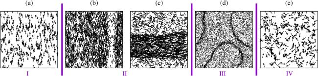
Figure 5. Steady-state snapshots. (a) Nematic phase with a noise of 0.08. (b), (c) Nematic band phase with the coexistence of the low-density disordered region and the high-density band with a noise of 0.1 and 0.13, respectively. (d) Chaotic thin band phase with a noise of 0.168. (e) Disordered phase with a noise of 0.2. Images adopted from [88]. |
For active nematics, in the INT induced by increasing density, Shi et al [154], observed the coexistence of dense nematic bands and isotropic gas, as illustrated in figures 6(a), (b) and (c). Considering the hydrodynamic description, the chaotic phase coexistence arises from the instabilities of the rotational and nematic band solutions. Half-integer and full-integer defects can coexist [155]. There is also spatial coexistence and switching between turbulent and nematic phases interfaced with a passive liquid crystal [156].
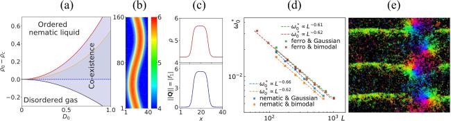
Figure 6. (a) Phase diagram in the $\left({D}_{0},{\rho }_{0}\right)$ plane, where ${D}_{0}=\left({D}_{\parallel }-{D}_{\perp }\right)/\left({D}_{\parallel }+{D}_{\perp }\right)$, ${D}_{\parallel }$ and ${D}_{\perp }$ are the longitudinal and transversal diffusion constants, respectively, and ${\rho }_{0}$ is the density. The black and red solid lines represent the binodal lines, while the dashed blue and dashed yellow lines indicate the spinodal lines. (b) Color maps depicting the density field, showing that the coexistence phase is unstable and the dense nematic bands are chaotic. (c) Density and nematic orders of the band solutions of continuum models. (d) The maximum noise strength ${\omega }_{0}^{\ast }$ for polar or nematic phase is a function of system size L, where ferro means polar alignment. (e) Snapshot of the phase coexistence between bands, rotational vortices, and disordered gas. Images adopted from [71, 154]. |
At low chirality, phase coexistence exists in the active matter composed of either chiral polar particles or chiral self-propelled rods [53, 71, 157]. In an infinite-size system, the polar and nematic phases are unstable to any degree of chirality with zero-mean Gaussian distribution, symmetric bimodal distribution, or unimodal distribution, as illustrated in figures 6(d) and (e), while the band phase remains robust. At high chirality, chiral polar particles self-organize into dense clouds [158]. The rotating-packets phase with a rotating global polarity and the rotational-vortices phase are found in experiments [159–161] and simulations for active semiflexible filaments [162], or curved active polymers [34]. The macrodroplet phase, rotational-vortices phase, and rotating-packets phase represent a form of microphase separation, where the number of patterns increases with density, aligning with continuum theories. Depending on initial conditions, the macrodroplet phase and the rotating-packets phase can coexist at moderate chirality. Rotating packets exhibit chirality-sorting, a self-sorting phenomenon observed in experiments [163]. For nematic chiral particles, nematic-vortices phase and active-foams phase are observed [71].
4.3. Hysteresis
Hysteresis, another feature of discontinuous phase transition, occurs when the noise is first increased and then decreased in the VLM, as shown in figure 4(f). At the phase transition point, the order parameter for the increasing-noise process exceeds that for the decreasing-noise process. The process of increasing density exhibits hysteresis during the discontinuous phase transitions from the reverse-band phase to the disordered phase [164]. In the reverse-band phase, low-density particles align and move, while high-density bands remain locally stationary. This phenomenon was initially observed in a model of collective cell migration [165], and linked to the density waves seen in traffic flow [166]. Hysteresis is also observed during expansion and compression of self-propelled rods when varying the packing fraction [151].
5. Topological phase transitions
In equilibrium, topological phase transitions typically involve changes in topological invariants or defects, such as Chern numbers [167]. Topological invariants are stable configurations that remain unchanged under smooth transformations and typically emerge during topological phase transitions. Topological defects appear to be irregularities or discontinuities in the order parameter, such as dislocations in crystalline materials [168]. The topological charge𝑘 of a disclination is an important topological invariant that quantifies the angular mismatch around the defect core, as depicted in figure 7. The topological charge is determined by
$\begin{eqnarray}k=\displaystyle \frac{1}{2\pi }\oint {\rm{d}}{\theta }_{n},\end{eqnarray}$
where ${\theta }_{{\rm{n}}}$ is the orientational angle of the rod-like molecule, and the integral encircles the disclination point counterclockwise [169]. The motion of topological defects can lead to the phase transition. The BKT [170, 171] phase transition is induced by the binding and unbinding of topological defects known as vortices (+1 defect and −1 defect), which is observed for the XY model, 2D liquid crystals [172], superfluid helium films [173], and thin film superconductors [174]. At low temperatures, the correlation function exhibits a power-law decay, and vortex-antivortex pairs appear, indicating quasi-long-range order. This behavior arises from the effective attraction between opposite charge pairs. As temperature increases to approach the transition point, thermal fluctuations intensify, leading to the unbinding of these pairs, and the correlation length exhibits exponential divergence [175], leading to a proliferation of free vortices. At high temperatures, short-range order exists and the correlation function decays exponentially. In liquid crystal, topological defects of nematic particles anneal to minimize the free energy, and eventually form an ordered nematic phase.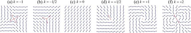
Figure 7. Configurations of topological defects in nematic systems. The blue arrows denote particle orientations and red arrows indicate defect orientations. The configurations of (a)–(f) have different defect charges k. Images adopted from [169]. |
For high-density DAAM, strong interactions and geometric properties of asymmetrical particle shape enhance the formation of topological defects. Creation, annihilation, and coordinate motion of topological defect pairs can drive non-equilibrium topological phase transition, which may be related to the control of multicellular organization and tissue mechanics. The geometric structure of topological defects determines their motion characteristics; for example, only +1/2 defect has a local asymmetric geometric polarity and is motile, as shown in figure 7.
Weber et al [40], have studied the phase transitions of polar particles at high densities. The velocity of particle $i$ is updated by ${{\boldsymbol{v}}}_{i}\left(t+{\rm{\Delta }}t\right)\,=\,$${v}_{{\rm{o}}}\displaystyle {\sum }_{\left|{{\boldsymbol{r}}}_{i}-{{\boldsymbol{r}}}_{j}\right|\lt R}\left({{\boldsymbol{v}}}_{j}\left(t\right)/\left|{{\boldsymbol{v}}}_{j}\left(t\right)\right|\right)/\left|\displaystyle {\sum }_{\left|{{\boldsymbol{r}}}_{i}-{{\boldsymbol{r}}}_{j}\right|\lt R}\left({{\boldsymbol{v}}}_{j}\left(t\right)/\left|{{\boldsymbol{v}}}_{j}\left(t\right)\right|\right)\right|$ $+{v}_{{\rm{r}}}\displaystyle {\sum }_{\left|{{\boldsymbol{r}}}_{i}-{{\boldsymbol{r}}}_{j}\right|\lt R}\left({{\boldsymbol{r}}}_{i}\left(t\right)-{{\boldsymbol{r}}}_{j}\left(t\right)\right)/\left|{{\boldsymbol{r}}}_{i}\left(t\right)-{{\boldsymbol{r}}}_{j}\left(t\right)\right|$, where ${v}_{{\rm{o}}}$ is the strength of the orientational forces and ${v}_{{\rm{r}}}$ is the strength of the repulsive forces. The relative strength of repulsive and orientational forces induces a transition from the polar phase with line defect to an active hexagonal close-packed crystal phase, as shown in figure 8. The polar phase is distinguished by the collective movement of polycrystalline structures, accompanied by excitations resembling sound waves. In contrast, the active crystal phase represents a defect-free state characterized by long-range bond-orientational hexatic order parameter ${\Psi }_{6}\,=\left\langle {\left|{{\mathscr{N}}}_{i}\right|}^{-1}{\sum }_{j\in {{\mathscr{N}}}_{i}}{{\rm{e}}}^{{\rm{i}}6{\theta }_{ij}}\right\rangle $ and quasi-long-range translational order of the correlation function ${C}_{{\boldsymbol{G}}}\left(r\right)={\left({\sum }_{i}{\left|{{\rm{e}}}^{-{\rm{i}}{\boldsymbol{G}}\cdot {{\boldsymbol{r}}}_{i}}\right|}^{2}\right)}^{-1}{\sum }_{\left|{{\boldsymbol{r}}}_{i}-{{\boldsymbol{r}}}_{j}\right|=r}{{\rm{e}}}^{-{\rm{i}}{\boldsymbol{G}}\cdot \left({{\boldsymbol{r}}}_{i}-{{\boldsymbol{r}}}_{j}\right)}$, where ${{\mathscr{N}}}_{i}$ is the number of Voronoi neighbors of particle i, ${\theta }_{ij}$ is the bond angle between particles i and j, and ${\boldsymbol{G}}$ denotes the reciprocal lattice vector. Topological defects in the active crystal phase contract with each other and self-annihilate. During the phase transition, there is a proliferation of topological defects, as shown in figure 8(d). By both experiment and simulation, Copenhagen et al [176], have investigated the transition of malignant cancer cells induced by the creation and annihilation of topological defects, and found that different phases exhibit distinct distributions of topological defect pairs with opposite velocity directions. In polar active matter, both half- and full-integer topological defects can emerge [155]. The annihilation of defect pairs leads to a transition from the polar phase to the rotating phase with an effective repulsive interaction between defect pairs.
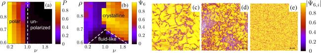
Figure 8. Polar order parameter $P$ (a) and hexatic order parameter ${{\rm{\Psi }}}_{6}$ (b) as functions of the packing fraction $\rho $ as well as the ratio between the repulsive and orientational forces $\nu ={v}_{{\rm{r}}}/{v}_{{\rm{o}}}$. The dashed white lines indicate tentative phase boundaries with $P=0.2$ and ${{\rm{\Psi }}}_{6}=0.2$. (c) Aligned dislocations forming a network without well-defined grain boundaries with $v=0.25$. (d) Assembled dislocations with $v=0.75$. (e) Hexatic crystal with $v=1.5$. The packing fraction $\rho =0.85$ for (c), (d) and (e). Images adopted from [40]. |
Similar to 2D XY model, active nematics at high densities undergo a BKT-like phase transition with increasing noise, resulting in continuous symmetry breaking [177]. At low noise levels, the orientational spatial correlation functions decay algebraically, while they decay exponentially in the disordered phase. The correlation length diverges as the system approaches the critical point. Instabilities at large wavelengths [178], lead to spontaneous nucleation and unbinding of defects, which can disrupt the long-range nematic order [179–181]. In experiments, as density increases, elongated cells change from a disordered phase to a nematic phase, where trapped topological defects prevent the formation of a perfectly ordered nematic phase [182]. On a spherical surface, transitions between different phases characterized by defect trajectories are induced by elastic forces [183].
The effective interaction between topological defects affects the ordered state of active nematics. A disclination with a charge of +1/2 exhibits polarization, causing an unbalanced stress field around the defect and resulting in axial migration [184]. By contrast, −1/2 defects typically display a 'three-arm' symmetry with more erratic motion and slower diffusion than +1/2 defects [11]. When pairs of −1/2 and +1/2 defects come into proximity, they can annihilate each other [185], thereby reducing the system's energy. Considering the collective motion of +1/2 defects, increasing density induces a phase transition of defects from the ordered polar phase to an isotropic phase, as shown in figure 9. This observation may suggest the presence of an effective polar force between +1/2 defects. We can measure the defect nematic order parameter ${S}_{{\rm{defect}}}=\left\langle \cos \left(2\left(\psi -\left\langle \psi \right\rangle \right)\right)\right\rangle $ and the defect polar order parameter $P=\left\langle \cos \left(\left(\psi -\left\langle \psi \right\rangle \right)\right)\right\rangle $, where $\psi $ is the velocity orientation of the +1/2 defect. As a +1/2 defect moves across the system, it reorients the local nematic field by approximately 90 degrees in its track. The defect order parameters can thus be used to quantify the degree of alignment of both defect motion and the nematic field. Unlike in equilibrium lyotropic liquid crystals, where order typically increases with density, here the defect order parameters decrease continuously as the density increases, suggesting a possible continuous phase transition. There are two types of particle collisions: one that promotes nematic order and one that inhibits it [186]. At low densities, based on a modified Smoluchowski equation, the angular information exchanged during collisions persists long enough to facilitate the nematic order [66]. However, at high densities, the linear instability of bending deformations causes a breakdown of the nematic order. Exploring the scaling laws and universal behaviors of these non-equilibrium behaviors remains an important direction for future research. In circular confinement, a transition to anisotropic flow with ±1 defects occurs when the elastic interactions between defects become dominant [187].
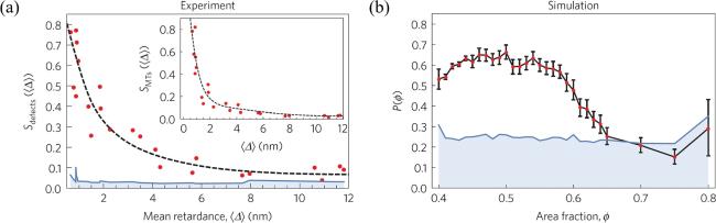
Figure 9. (a) Defect nematic order parameter ${S}_{{\rm{defects}}}$ increases as the mean retardance, which is positively correlated with density, decreases in experiments. The blue shaded region represents the 'noise floor.' (b) Defect polar order parameter $P$ increases as density decreases in simulations. The distinctions between nematic and polar orders may arise from the bend modulus difference, boundary conditions difference, and the effects of hydrodynamic interactions. Images adopted from [185]. |
Topological defects play a significant role in active nematics, such as densely packed cell layers, influencing and regulating various biological functions [188]. In monolayers of Madin Darby canine kidney epithelia, excess cells are vertically extruded at +1/2 defects and die [189], driven by the mechanical stresses. The dynamics of topological defects contribute to shape changes in growing colonies of dividing cells, by interacting with the interface at a specific interaction range [190]. Topological defects influence the density of cultured stem cells, with cells concentrating at +1/2 defects and escaping from −1/2 defects, arising from the interplay between the anisotropic friction and the active force [184].
Chirality introduces two distinct symmetry-breaking properties to DAAM: odd viscosity, characterized by an asymmetric viscosity tensor [191], and stress chirality, characterized by the asymmetric shear stress. Characterized by an ultraviolet divergence in the hydrodynamic field theory, a topological transition is marked by a sign change in odd viscosity without closing the bulk gap [192]. However, the intrinsic rotation of chiral active nematics [193], suppresses the defect separation that drives chaotic flows in non-rotating active fluids. This suppression explains the circular motion observed in the organization of sperm cells [159] and bacteria [30]. Stress chirality of monolayers of nematic cells [39] influences the dynamics of topological defects, and the transition from a polar phase to a disordered phase can be deduced through particle-image-velocimetry measurements and the classical pitchfork bifurcation.
6. Conclusions and outlook
The non-equilibrium characteristics of active matter, including the coupling of local density and mean velocity, as well as the emergence of various patterns, clusters, active topological defects, and abnormal fluctuations, may have influence on their phase transitions. The phase behavior of polar particles, self-propelled rods, and active nematics increases in complexity. However, in the ordered phase, they share a common characteristic known as giant number fluctuations,which refers to significant particle number fluctuations $\sqrt{\left\langle {\left(n-\left\langle n\right\rangle \right)}^{2}\right\rangle }\propto {\left\langle n\right\rangle }^{\alpha },\alpha \gt 0.5$ in subsystems, consistent with the results from the Toner–Tu equation [55], for polar particles. Additionally, the fluctuations of the disordered phase of DAAM conform to the equilibrium theory.
In this review, we summarize the non-equilibrium phase transition characteristics of dry aligning active matter, including polar particles, self-propelled rods, active nematics, and their chiral counterparts, along with combined theoretical tools of macroscopic (analytical) and microscopic (computational) models. Based on the understanding of equilibrium phase transitions, continuous, discontinuous, and topological phase transitions of dry aligning active matter are discussed and debated. The Vicsek model is likely to display discontinuous phase transitions at high particle velocities and continuous phase transitions at low particle velocities. A tri-critical point may exist at intermediate velocities, which separates the continuous and discontinuous phase transitions. Furthermore, this active system could exhibit both continuous and discontinuous phase transitions simultaneously [47]. In non-equilibrium critical phenomena, the diversity of universality categories increases significantly, and these diversities are often influenced by various symmetric properties [194].
Other phase transitions may also occur in DAAM. The mixed-order phase transitions, also referred to as the hybrid phase transitions, combine the characteristics of both first-order and second-order phase transitions. Systems with long-range interactions exhibit mixed-order traits, as seen in examples such as the one-dimensional Ising model [195–197], the percolation transition [198], and the jamming transition [199] in complex networks, and the DNA denaturation transition [200], where the order parameter is discontinuous while the correlation length diverges. The mixed-order phase transitions can also occur in active matter. For momentum-conserving polar particles, the polar order is continuous at the phase transition point, whereas the high density moving clusters coexist with disordered gas [89]. The substantial increases in pressure and shear viscosity, along with slower structural and mechanical relaxations, suggest a type of glass transition towards an internally glassy, solid-like structure, akin to experimental systems involving self-propelled colloids [201].
Considering the heterogeneous nature of particles and their environment, which can be complex, confined, or crowded [202], it is crucial to assess the robustness and stability of phases. Any level of quenched disorder renders the polar phase unstable [203], while heterogeneous alignment ability [204] and speed inhomogeneity [205] can significantly influence phase transition behaviours. The transition between order and disorder can be triggered by various phenomena, such as the growth and spreading of dense cell colonies [206], the vibrations of granular rods [25, 207], as well as factors like density, length-to-width ratio, and boundary conditions of self-propelled rods [66, 208]. Artificial active matter, including colloids driven by catalytic reactions, represents functional nanomachines capable of precise manipulation at the nanoscale in response to external stimuli [209]. However, the fundamental nature of these transitions remains unclear.
Beyond dry active matter, hydrodynamic interactions in wet active matter may have significant influences on phase transitions. The transition from nematic phase to turbulence in active nematic particles suggests the existence of universal scaling laws and universality classes [43, 210, 211], primarily influenced by hydrodynamic interactions. The breaking of the SO(2) symmetry characterizes the transition from the defect-free active turbulence to the active turbulence with topological defects, related to fast decay of the two-point correlation [212]. Exploring the interplay between active turbulence and phase transitions is a compelling area of study. In extensile active nematics, internal activity generates forces that push particles apart along their axis, contrasting with contractile systems. The nematic order parameter and bond-orientational order parameter of active contractile polar filaments undergo a discontinuous phase transition induced by increasing active temperature, shifting from a quasi-long-range ordered solid with tetradic order to a bond-nematic liquid phase [213]. Conversely, the transition from a moving aster street to a stationary aster lattice remains continuous with increasing density of filaments and motors. Active backflow [214], induced by active stresses enhances the annihilation dynamics by speeding up the defect motion towards each other [179], for contractile systems. Conversely, in extensile microtubules and kinesin assemblies [180], defect pairs are driven apart [215], leading to defect proliferation. Polar-isotropic [216–218], and nematic–isotropic [219], transition occurs in active gels, while polar and nematic order are unstable in low Reynolds numbers ($\mathrm{Re}\ll 1$) where viscosity dominates [178].
The prospective applications of active matter are very broad, spanning biomedical fields, unmanned aerial vehicles (UAVs), soft robotics [220], self-healing materials [221], and smart materials [222]. For instance, collective behavior of bacteria and cells in biomedicine can help develop new treatments and drug delivery systems by using E. coli bacterium [223], and clusters of autonomously moving robots or UAVs can be programmed to perform tasks through coordinated collective behavior [224, 225]. Signaling mechanisms, whether through biochemical pathways in cellular biology or within bacterial colonies, or via external stimuli-like food, sound, smell, or light for animal systems, are pivotal in both inducing and regulating phase transitions in active matter. By enhancing communication and coordination among constituent units, signaling mechanisms facilitate transitions between distinct phases. This functionality is crucial in various biological processes such as tissue growth, morphogenesis, biofilm formation, wound healing, as well as in pathological conditions like cancer growth and metastasis [209].
Exploring the physical mechanisms of DAAM may unveil novel principles in the non-equilibrium statistical physics. DAAM exhibits distinctly non-equilibrium characteristics with phase transition mechanisms that are highly intricate and not fully elucidated. The Ginzburg–Landau free energy functional of continuum models accurately predicts temperature dependence near continuous phase transition points, but its predictive capability across the entire phase diagram is limited because the consideration of activity is not theoretically rigorous [226]. Therefore, advancing a universal theory for non-equilibrium phase transitions represents a promising avenue for future research. Precisely linking simulation and continuum models, along with developing models that can explain and regulate biological functions, is also a key future direction.