Welcome to visit Communications in Theoretical Physics,
Mathematical Physics

Rogue wave patterns in the nonlinear Schrödinger-Boussinesq system

  • Xiaoyu Cheng ,
  • Qing Huang
Expand
  • School of Mathematics, Northwest University, Xi’an, 710127, China

Received date: 2024-11-06

  Revised date: 2025-01-16

  Accepted date: 2025-01-26

  Online published: 2025-04-07

Copyright

© 2025 Institute of Theoretical Physics CAS, Chinese Physical Society and IOP Publishing. All rights, including for text and data mining, AI training, and similar technologies, are reserved.
This article is available under the terms of the IOP-Standard License.

Cite this article

Xiaoyu Cheng , Qing Huang . Rogue wave patterns in the nonlinear Schrödinger-Boussinesq system[J]. Communications in Theoretical Physics, 2025 , 77(7) : 075004 . DOI: 10.1088/1572-9494/adae70

1. Introduction

Rogue waves are a kind of interesting solutions in nonlinear wave systems, which ’come from nowhere and disappear with no trace’ [1]. In other words, they generate from a constant (uniform) background, run to high amplitudes, and then return to the same background. Rogue waves which were initially explored in oceanography and later observed in the field of optics, have garnered significant attentions in recent years within the broader realm of physics and nonlinear wave studies. Especially in the field of integrable nonlinear wave systems, rogue waves have become a focal point of extensive research because of their mathematical novelty, physical significance and explicit analytical expressions. For rogue waves, the simplest (lowest-order) analytical solution was given for the nonlinear Schrödinger (NLS) equation by Peregrine [2]. This solution begins with a constant amplitude background and evolves into a peak three times the background height before decaying back into the background. Higher-order rogue waves were discovered subsequently [3-5]. In addition, rogue waves have been successfully identified in numerous integrable systems, including the coupled NLS equation [6-8], the Manakov system [9-11], and the Davey-Stewartson equations [12, 13] and so on.
The Kadomtsev-Petviashvili (KP) reduction technique, a very powerful tool for constructing localized waves of integrable systems, has been used to build up higher-order rogue wave solutions of many integrable systems, such as NLS equation [4, 14], Boussinesq equation [15], three-wave resonant interaction systems [16] and nonlinear Schrödinger-Boussinesq (NLS-Boussinesq) equation [17]. Owing to the intricate and diverse dynamic behaviors of higher-order rogue wave solutions, there has been increasing interest in classifying their structures. This classification enables the prediction of subsequent rogue wave structures based on the initial ones. Numerous patterns of higher-order rogue wave solutions including triangular, circular, pentagram, heptagram, circle-arc, double-column and many other structures for the NLS equation [3, 18-20], and modified-triangle, circle-triangle and multi-circle patterns for the derivative NLS equation [21] have been obtained. Meanwhile, the connection between predicted rogue wave patterns for NLS equation and the root structures of Yablonskii-Vorob’ev polynomials was established [14], which reveals the presence of more complex rogue wave patterns and more importantly makes it possible to predict complex patterns in higher-order rogue waves. What’s more, in [14] the predicted solutions were used to analyze the dynamic behaviors of the rogue waves since they showed excellent agreement with the true ones. Shortly afterwards similar connections have been identified for the derivative NLS equation [10], the Boussinesq equation [10], the Manakov system [10], the KP equation [22, 23] and many other systems. Very recently, the rogue wave patterns are related to the root structures of the Adler-Moser polynomials with purely simple roots in [24, 25] and with multiple roots in [26], leading to the discovery of new rogue wave patterns.
In this paper, we consider the rogue wave patterns of the coupled NLS-Boussinesq system
$\begin{eqnarray}\begin{array}{c}\left\{\begin{array}{c}{\rm{i}}{{\rm{\Phi }}}_{t}-{{\rm{\Phi }}}_{{xx}}-u{\rm{\Phi }}=0,\\ {u}_{{xx}}+{u}_{{xxxx}}+3{({u}^{2})}_{{xx}}-3{u}_{{tt}}+{(|{\rm{\Phi }}{|}^{2})}_{{xx}}=0,\end{array}\right.\end{array}\end{eqnarray}$
which was first given in [27], where Ø(x, t) is a complex function and u(x, t) is a real function. This system is recognized for describing the nonlinear propagation of coupled Langmuir and dust-acoustic waves in a multi-component dusty plasma, including some ions, electrons and charged dust particles. The amplitude of the Langmuir wave can be controlled by the NLS equation under conditions of slow modulation. While for small amplitude but finite amplitude ion-acoustic waves, it must be controlled by the driven Boussinesq equation to show bidirectional propagation. There has been a substantial amount of research on soliton solutions for the NLS-Boussinesq system. Its complete integrability was studied from the view of Painléve analysis [28] and N-soliton solutions were derived [29]. A hierarchy of rational solutions, Peregrine breathers and second-order rational solutions were given by using Hirota technique in [30]. Using KP hierarchy reduction technique, general higher-order rogue waves of the system (1) were constructed when the corresponding algebraic equation has a non-imaginary simple root [17]. Additionally, more general rogue wave expressions were provided for cases with a simple root and two simple roots and for the unique large parameter case the rogue wave patterns are determined by the root structure of the Yablonskii-Vorob’ev polynomial hierarchy [31]. Here we aim to predict the rogue wave patterns of system (1) for multiple large parameters, based on the root structure of Adler-Moser polynomials and the approach developed in [24].
The outline of this paper is as follows. In section 2, rogue wave solutions for system (1) are presented. In section 3, for illustration, we display the figures of the first-order, second-order and third-order rogue waves. In section 4, the detailed analytical predictions and shapes of rogue wave patterns for system (1) are provided. Since the predicted solutions coincide with the corresponding true solutions, rogue wave patterns can be predicted efficiently. The last section contains the concluding remarks and brief discussion of the results obtained.

2. General rogue wave solutions

The bilinear equations of system (1) is [17]
$\begin{eqnarray}\begin{array}{rcl}({\rm{i}}{D}_{t} & - & 2{\rm{i}}\alpha {D}_{x}-{D}_{x}^{2})g\cdot f=0,\\ ({D}_{x}^{4} & + & {D}_{x}^{2}-3{D}_{t}^{2}-1)f\cdot f+| g{| }^{2}=0,\end{array}\end{eqnarray}$
which associates with (1) by the transformation
$\begin{eqnarray}{\rm{\Phi }}={{\rm{e}}}^{{\rm{i}}(\alpha x+{\alpha }^{2}t)}\frac{g}{f},\,\,\,\,u=2{{\rm{\partial }}}_{x}^{2}{\rm{ln}}f,\end{eqnarray}$
where α represents an arbitrary real constant, f and g are real and complex functions respectively. Here D is the Hirota’s bilinear differential operator defined by [32]
$\begin{eqnarray*}\begin{array}{l}F({D}_{x},{D}_{y},{D}_{t},\cdots \,){G}_{1}(x,y,t,\cdots \,){G}_{2}(x,y,t,\cdots \,)\\ =\,F({\partial }_{x}-{\partial }_{{x}^{{\prime} }},{\partial }_{y}-{\partial }_{{y}^{{\prime} }},{\partial }_{t}-{\partial }_{{t}^{{\prime} }},\cdots \,){G}_{1}(x,y,t,\cdots \,)\\ {\,\times \,G}_{2}({x}^{{\prime} },{y}^{{\prime} },{t}^{{\prime} },\cdots \,){| }_{{x}^{{\prime} }=x,{y}^{{\prime} }=y,{t}^{{\prime} }=t,\cdots },\end{array}\end{eqnarray*}$
where F is a polynomial of Dx, Dy, Dt, ... and Gi are differentiable functions of their arguments x, y, t, ... .
To ensure the completeness of the paper and facilitate our discussion of rogue wave patterns with multiple large parameters, we briefly introduce the related basic results of rogue wave solution of system (1) in [31], which involve the Schur polynomials Sj(x) with x = (x1, x2,...) defined as
$\begin{eqnarray}\displaystyle \sum _{j=0}^{\infty }{S}_{j}({\boldsymbol{x}}){\epsilon }^{j}=\exp \left(\displaystyle \sum _{k=1}^{\infty }{x}_{k}{\epsilon }^{k}\right),\end{eqnarray}$
or more explicitly,
$\begin{eqnarray*}{S}_{j}({\boldsymbol{x}})=\displaystyle \sum _{{l}_{1}+2{l}_{2}+\cdots +m{l}_{m}=j}\left(\displaystyle \prod _{k=1}^{m}\displaystyle \frac{{x}_{k}^{{l}_{k}}}{{l}_{k}!}\right),\,\,\,\,\,\,\,j\geqslant 0,\end{eqnarray*}$
and Sj(x) ≡ 0 for j < 0. Since only the case (ρ, h) = (1, 0) for the rogue wave dynamics is considered in [31]. Here, following [31] we present the rogue wave solutions with their specific choice of (ρ, h).

[31] If p0 is a non-imaginary simple root of the algebraic equation ${{ \mathcal Q }}^{{\prime} }(p)=0$ with ${ \mathcal Q }(p)={p}^{3}+\frac{p}{4}\,-\frac{1}{8(p-{\rm{i}}\alpha )}$, the NLS-Boussinesq system (1) under boundary condition

$\begin{eqnarray*}({\rm{\Phi }}(x,t),u(x,t))\to ({{\rm{e}}}^{{\rm{i}}(\alpha x+{\alpha }^{2}t)},0),\,\,\,\,x,t\to \infty \end{eqnarray*}$
admits Nth order rogue wave solutions
$\begin{eqnarray}\begin{array}{rcl}{{\rm{\Phi }}}_{N}(x,t) & = & {{\rm{e}}}^{{\rm{i}}(\alpha x+{\alpha }^{2}t)}\frac{{\sigma }_{1}}{{\sigma }_{0}},\\ {u}_{N}(x,t) & = & 2{{\rm{\partial }}}_{x}^{2}{\rm{ln}}{\sigma }_{0},\,\,\,\,\,\,\,N\in {{\mathbb{Z}}}^{+},\end{array}\end{eqnarray}$
where
$\begin{eqnarray*}{\sigma }_{n}=\mathop{\det }\limits_{1\,\leqslant \,i,j\,\leqslant \,N}({m}_{2i-1,2j-1}^{(n)}),\end{eqnarray*}$
with
$\begin{eqnarray*}{m}_{ij}^{(n)}=\displaystyle \sum _{\nu =0}^{\min (i,j)}{\left(\displaystyle \frac{| {p}_{1}{| }^{2}}{{({p}_{0}+{p}_{0}^{* })}^{2}}\right)}^{\nu }{S}_{i-\nu }({{\boldsymbol{x}}}^{+}+\nu {\boldsymbol{s}})\,{S}_{j-\nu }({{\boldsymbol{x}}}^{-}+\nu {{\boldsymbol{s}}}^{* }).\end{eqnarray*}$
Here s = (s1, s2,...) is defined by
$\begin{eqnarray*}\mathrm{ln}\left(\displaystyle \frac{1}{k}\displaystyle \frac{{p}_{0}+{p}_{0}^{* }}{{p}_{1}}\displaystyle \frac{p(k)-{p}_{0}}{p(k)+{p}_{0}^{* }}\right)=\displaystyle \sum _{r=1}^{\infty }{s}_{r}{k}^{r},\end{eqnarray*}$
with ${p}_{1}={p}^{{\prime} }(0)$, p(k) which satisfies the equation
$\begin{eqnarray*}{{ \mathcal Q }}_{1}(p(k))={{ \mathcal Q }}_{1}({p}_{0})\cosh (k),\end{eqnarray*}$
and the vectors ${{\boldsymbol{x}}}^{\pm }=({x}_{1}^{\pm },0,{x}_{3}^{\pm },0,\cdots \,{,}0,{x}_{2r+1}^{\pm },0,\cdots \,)$ are defined by
$\begin{eqnarray*}\begin{array}{rcl}{x}_{2r+1}^{+} & = & {\alpha }_{2r+1}x-{\beta }_{2r+1}{\rm{i}}t+n{\vartheta }_{2r+1}+{a}_{2r+1},\\ {x}_{2r+1}^{-} & = & {\alpha }_{2r+1}^{* }x+{\beta }_{2r+1}^{* }{\rm{i}}t-n{\vartheta }_{2r+1}^{* }+{a}_{2r+1}^{* },\end{array}\end{eqnarray*}$
with complex constants αr, βr, νr given by
$\begin{eqnarray*}\begin{array}{rcl}p(k)-{p}_{0} & = & \displaystyle \sum _{r=1}^{\infty }{\alpha }_{r}{k}^{r},\\ {p}^{2}(k)-{p}_{0}^{2} & = & \displaystyle \sum _{r=1}^{\infty }{\beta }_{r}{k}^{r},\\ \mathrm{ln}\frac{p(k)-{\rm{i}}\alpha }{{p}_{0}-{\rm{i}}\alpha } & = & \displaystyle \sum _{r=1}^{\infty }{\vartheta }_{r}{k}^{r},\end{array}\end{eqnarray*}$
and a1 = 0, a2r+1 are arbitrary complex constants.

3. Dynamics of general rogue wave solutions

The dynamical properties of the higher-order rogue wave solutions given in Lemma 1 can be further analyzed, where α and a2r+1 play the extremely vital roles.

3.1. The first-order fundamental rogue wave

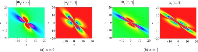
Selecting N = 1 in equation (5), the first-order fundamental rogue wave is written as
$\begin{eqnarray}\begin{array}{rcl}{{\rm{\Phi }}}_{1}(x,t) & = & {{\rm{e}}}^{{\rm{i}}(\alpha x+{\alpha }^{2}t)}{\hat{{\rm{\Phi }}}}_{1}(x,t),\\ {\hat{{\rm{\Phi }}}}_{1}(x,t) & = & \frac{({p}_{1}x-2{p}_{0}{p}_{1}{\rm{i}}t+{\vartheta }_{1})({p}_{1}^{\ast }x+2{p}_{0}^{\ast }{p}_{1}^{\ast }{\rm{i}}t-{\vartheta }_{1}^{\ast })+{\zeta }_{0}}{|{p}_{1}x-2{p}_{0}{p}_{1}{\rm{i}}t{|}^{2}+{\zeta }_{0}},\\ {u}_{1}(x,t) & = & 2{{\rm{\partial }}}_{x}^{2}{\rm{ln}}(|{p}_{1}x-2{p}_{0}{p}_{1}{\rm{i}}t{|}^{2}+{\zeta }_{0}),\end{array}\end{eqnarray}$
where ${\vartheta }_{1}=\frac{{p}_{1}}{{p}_{0}-{\rm{i}}\alpha },\,{\zeta }_{0}=\frac{| {p}_{1}{| }^{2}}{{({p}_{0}+{p}_{0}^{* })}^{2}}.$ For illustration, we only give the first-order rogue waves in two cases with respect to α, as shown in figure 1: (i) p0 = δ1 with α = 0; (ii) p0δ2 with $\alpha =\frac{1}{2}$, where ${\varrho }_{1}=\frac{\sqrt{6\sqrt{6}-3}}{12}+\frac{\sqrt{6\sqrt{6}+3}}{12}\,{\rm{i}}$ and δ2 = 0.27540 + 0.64170 i.
Figure 1. The first-order rogue waves of NLS-Boussinesq system.

3.2. The second-order rogue wave

Taking N = 2 in equation (5), the second-order rogue wave of NLS-Boussinesq system is given by
$\begin{eqnarray}\begin{array}{rcl}{{\rm{\Phi }}}_{2}(x,t) & = & \frac{{\sigma }_{1}}{{\sigma }_{0}}{{\rm{e}}}^{{\rm{i}}(\alpha x+{\alpha }^{2}t)},\\ {u}_{2}(x,t) & = & 2{{\rm{\partial }}}_{x}^{2}{\rm{ln}}({\sigma }_{0}),\end{array}\end{eqnarray}$
where
$\begin{eqnarray*}\begin{array}{rcl}{\sigma }_{n} & = & \left(\right.{({x}_{10}^{+})}^{3}-3{x}_{10}^{+}{({x}_{11}^{+})}^{2}+6{x}_{10}^{+}{x}_{20}^{+}-6{x}_{10}^{+}{x}_{21}^{+}+6{x}_{30}^{+}\left)\right.\\ & & \times \left(\right.{({x}_{10}^{-})}^{3}-3{x}_{10}^{-}{({x}_{11}^{-})}^{2}+6{x}_{10}^{-}{x}_{20}^{-}-6{x}_{10}^{-}{x}_{21}^{-}+6{x}_{30}^{-}\left)\right.\\ & & +36{\zeta }_{0}({x}_{10}^{+}{x}_{10}^{-})({x}_{12}^{+}{x}_{12}^{-})+36{\zeta }_{0}^{2}({x}_{10}^{+}{x}_{10}^{-}+{x}_{12}^{+}{x}_{12}^{-})+6{\zeta }_{0}^{3},\\ n & = & 0,1,\end{array}\end{eqnarray*}$
with
$\begin{eqnarray*}\begin{array}{rcl}{x}_{j\nu }^{+} & = & {\alpha }_{j}x-{\beta }_{j}{\rm{i}}t+n{\vartheta }_{j}+\nu {s}_{j}+{a}_{j},\\ {x}_{j\nu }^{-} & = & {\alpha }_{j}^{* }x+{\beta }_{j}^{* }{\rm{i}}t-n{\vartheta }_{j}^{* }+\nu {s}_{j}^{* }+{a}_{j}^{* },\\ j & = & 1,2,3,\quad \nu =0,1,2.\end{array}\end{eqnarray*}$
Here
$\begin{eqnarray*}\begin{array}{rcl}{\alpha }_{n} & = & \frac{{p}_{n}}{n!},\quad {\beta }_{1}=2{p}_{0}{p}_{1},\quad {\beta }_{2}={p}_{1}^{2}+{p}_{0}{p}_{2},\\ {\beta }_{3} & = & {p}_{1}{p}_{2}+\frac{1}{3}{p}_{0}{p}_{3},\end{array}\end{eqnarray*}$
$\begin{eqnarray*}\begin{array}{rcl}{\vartheta }_{1} & = & \frac{{p}_{1}}{{p}_{0}-{\rm{i}}\alpha },\quad {\vartheta }_{2}=\frac{{p}_{2}}{2({p}_{0}-{\rm{i}}\alpha )}-\frac{{p}_{1}^{2}}{2{({p}_{0}-{\rm{i}}\alpha )}^{2}},\\ {\vartheta }_{3} & = & \frac{2{p}_{1}^{3}-3{p}_{1}{p}_{2}({p}_{0}-{\rm{i}}\alpha )+{p}_{3}{({p}_{0}-{\rm{i}}\alpha )}^{2}}{6{({p}_{0}-{\rm{i}}\alpha )}^{3}},\end{array}\end{eqnarray*}$
$\begin{eqnarray*}\begin{array}{rcl}{s}_{1} & = & \frac{({p}_{0}+{p}_{0}^{* }){p}_{2}-2{p}_{1}^{2}}{2{p}_{1}({p}_{0}+{p}_{0}^{* })},\\ {s}_{2} & = & \frac{12{p}_{1}^{4}-12{p}_{2}({p}_{0}+{p}_{0}^{* }){p}_{1}^{2}+4{p}_{3}{({p}_{0}+{p}_{0}^{* })}^{2}{p}_{1}-3{p}_{2}^{2}{({p}_{0}+{p}_{0}^{* })}^{2}}{24{({p}_{0}+{p}_{0}^{* })}^{2}{p}_{1}^{2}},\end{array}\end{eqnarray*}$
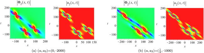
with ${p}_{n}=\frac{{{\rm{d}}}^{n}p(k)}{{\rm{d}}{k}^{n}}{| }_{k=0}$. Moreover, the solution (7) depends on not only α but also a3. To contrast with the first-order rogue waves shown in figure 1, α and p0 are chosen to be identical with those in section 3.1 and the corresponding second-order rogue wave patterns with a3 are displayed in figure 2.
Figure 2. The second-order rogue waves of NLS-Boussinesq system.

3.3. The third-order rogue wave

For N = 3 in equation (5), the third-order rogue wave of NLS-Boussinesq system is expressed as
$\begin{eqnarray}{{\rm{\Phi }}}_{3}(x,t)=\frac{{\sigma }_{1}}{{\sigma }_{0}}{{\rm{e}}}^{{\rm{i}}(\alpha x+{\alpha }^{2}t)},\,{u}_{3}(x,t)=2{{\rm{\partial }}}_{x}^{2}{\rm{ln}}({\sigma }_{0}),\end{eqnarray}$
where
$\begin{eqnarray*}{\sigma }_{n}=\mathop{\det }\limits_{1\,\leqslant \,i,j\leqslant 3}({m}_{2i-1,2j-1}^{(n)})=\left|\begin{array}{ccc}{m}_{11}^{(n)} & {m}_{13}^{(n)} & {m}_{15}^{(n)}\\ {m}_{31}^{(n)} & {m}_{33}^{(n)} & {m}_{35}^{(n)}\\ {m}_{51}^{(n)} & {m}_{53}^{(n)} & {m}_{55}^{(n)}\end{array}\right|.\end{eqnarray*}$
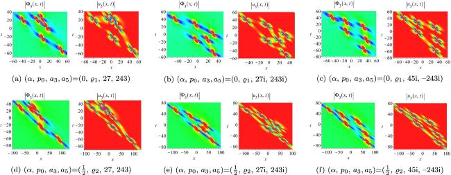
For the sake of brevity, the detailed expression of σn is not given here. It should be pointed out that the third-order rogue wave equation (8) contains (α, a3, a5) which will determine the rogue wave patterns. For illustration, the third-order rogue waves with (a3, a5) are displayed in figure 3. Here, taking figure 3(b) as an example, it exhibits the skewed heart-shaped structures for the third-order rogue wave with (α, p0, a3, a5) = (0, δ1, 27i, 243i) of system (1).
Figure 3. The third-order rogue waves of NLS-Boussinesq system.

4. Predictions for rogue wave patterns

The Nth order rogue waves of system (1) depend on parameters a3, a5,..., a2N-1. Rogue wave patterns have been predicted for a unique large parameter [31]. Now, we consider rogue wave patterns when there are multiple large parameters in equation (5) by means of Adler-Moser polynomials. We now briefly introduce the basic knowledge of Adler-Moser polynomials.
The Adler-Moser polynomials ΘN(z), proposed by Adler and Moser [33], were further formulated in [34] as
$\begin{eqnarray*}\begin{array}{rcl}{{\rm{\Theta }}}_{N}(z) & = & \displaystyle \prod _{j=1}^{N}(2j-1)!!\\ & & \times \left|\begin{array}{cccc}{\theta }_{1}(z) & {\theta }_{0}(z) & \cdots \, & {\theta }_{2-N}(z)\\ {\theta }_{3}(z) & {\theta }_{2}(z) & \cdots \, & {\theta }_{4-N}(z)\\ \vdots & \vdots & \vdots & \vdots \\ {\theta }_{2N-1}(z) & {\theta }_{2N-2}(z) & \cdots \, & {\theta }_{N}(z)\\ \end{array}\right|,\end{array}\end{eqnarray*}$
where θk(z) ≡ 0 if k < 0 and for k ≥ 0, θk(z) are Schur polynomials of the form
$\begin{eqnarray}\displaystyle \sum _{k=0}^{\infty }{\theta }_{k}(z){\epsilon }^{k}=\exp \left(z\epsilon +\displaystyle \sum _{i=1}^{\infty }{\kappa }_{i}{\epsilon }^{2i+1}\right),\end{eqnarray}$
with arbitrary complex constants κi.
When there is a unique nonzero parameter, Adler-Moser polynomials reduce to Yablonskii-Vorob’ev polynomials, and thus they are generalizations of Yablonskii-Vorob’ev polynomials. Adler-Moser polynomials are endowed by the existence of multi-parameter with much more diverse root structures than Yablonskii-Vorob’ev polynomials. Since a multiple root could split into simple roots upon a slight perturbation of parameters, without loss of any generality, we assume that ΘN(z), which is of degree $\frac{N(N+1)}{2}$, has $\frac{N(N+1)}{2}$ simple roots.
Assume that each parameter in {a3, a5,..., a2N-1} satisfies
$\begin{eqnarray}{a}_{2i+1}={\kappa }_{i}{A}^{2i+1},\quad 1\,\leqslant \,i\,\leqslant \,N-1,\end{eqnarray}$
where A ≫ 1, complex constants κi = O(1) and not all κi are zero. Now, we predict the patterns of the rogue wave solution (ØN(x, t), uN(x, t)).

If all roots of ΘN(z)=0 are simple, the Nth rogue wave (ØN(x, t), uN(x, t)) in equation (5) with large parameters (10) asymptotically separates into $\frac{N(N+1)}{2}$ fundamental rogue waves $({{\rm{e}}}^{{\rm{i}}(\alpha x+{\alpha }^{2}t)}{\hat{{\rm{\Phi }}}}_{1}(x-{\check{x}}_{0},t-{\check{t}}_{0}),{u}_{1}(x-{\check{x}}_{0},t-{\check{t}}_{0}))$ near $({\check{x}}_{0},{\check{t}}_{0})$, where $({\hat{{\rm{\Phi }}}}_{1}(x,t),{u}_{1}(x,t))$ satisfies equation (6) and its position $({\check{x}}_{0},{\check{t}}_{0})$ is given by

$\begin{eqnarray}\begin{array}{rcl}{\check{x}}_{0} & = & \frac{1}{{\rm{Re}}({p}_{0})}{\rm{Re}}\left(\frac{{\tilde{z}}_{0}A}{{p}_{1}}{p}_{0}^{\ast }\right)+{{\rm{\Delta }}}_{1},\\ {\check{t}}_{0} & = & -\frac{1}{2{\rm{Re}}({p}_{0})}{\rm{Im}}\left(\frac{{\tilde{z}}_{0}A}{{p}_{1}}\right)+{{\rm{\Delta }}}_{2},\end{array}\end{eqnarray}$
with ${\tilde{z}}_{0}$ being any of the $\frac{N(N+1)}{2}$ simple roots of ΘN(z) = 0 and 1, 2 are given by
$\begin{eqnarray}\begin{array}{rcl}{{\rm{\Delta }}}_{1} & = & -\frac{1}{{\rm{Re}}({p}_{0})}{\rm{Re}}\left(\frac{(N-1){s}_{1}}{{p}_{1}}{p}_{0}^{\ast }\right),\\ {{\rm{\Delta }}}_{2} & = & \frac{1}{2{\rm{Re}}({p}_{0})}{\rm{Im}}\left(\frac{(N-1){s}_{1}}{{p}_{1}}\right).\end{array}\end{eqnarray}$
The errors of these fundamental rogue waves are O(A-1). That is, when $\sqrt{{(x-{\check{x}}_{0})}^{2}+{(t-{\check{t}}_{0})}^{2}}=O(1)$, we get
$\begin{eqnarray*}\begin{array}{rcl}{{\rm{\Phi }}}_{N}(x,t) & = & {{\rm{e}}}^{{\rm{i}}(\alpha x+{\alpha }^{2}t)}{\hat{{\rm{\Phi }}}}_{1}(x-{\check{x}}_{0},t-{\check{t}}_{0})+O({A}^{-1}),\\ {u}_{N}(x,t) & = & {u}_{1}(x-{\check{x}}_{0},t-{\check{t}}_{0})+O({A}^{-1}).\end{array}\end{eqnarray*}$
For (x, t) which is not in the neighborhood of any of these fundamental waves, (ØN(x, t), uN(x, t)) asymptotically approaches the constant amplitude background $({{\rm{e}}}^{{\rm{i}}(\alpha x+{\alpha }^{2}t)},0)$ as A → + .

When parameters {a3, a5,..., a2N-1} satisfy equation (10) with A ≫ 1, we have

$\begin{eqnarray*}\begin{array}{rcl}{S}_{j}({{\boldsymbol{x}}}^{+}+\nu {\boldsymbol{s}}) & = & {S}_{j}(\tilde{{\boldsymbol{v}}})\,(1+O({A}^{-1})),\\ \tilde{{\boldsymbol{v}}} & = & ({p}_{1}x-2{p}_{0}{p}_{1}{\rm{i}}t,0,{\kappa }_{1}{A}^{3},0,{\kappa }_{2}{A}^{5},0,\cdots \,).\end{array}\end{eqnarray*}$
Note that νs1 term is much smaller than ${x}_{1}^{+}$, so it has no contribution to the leading-order term, thus we ignore the νs1 term in $\tilde{{\boldsymbol{v}}}$. By the relation (4) and (9), it is deduced that ${S}_{j}(\tilde{{\boldsymbol{v}}})={A}^{j}{\theta }_{j}(\tilde{z})$, $\tilde{z}={A}^{-1}({p}_{1}x-2{p}_{0}{p}_{1}{\rm{i}}t)$. Then we find that
$\begin{eqnarray*}\mathop{\det}\limits_{1\,\leqslant \,i,j\,\leqslant \,N}({S}_{2i-j}({{\boldsymbol{x}}}^{+}+\nu {\boldsymbol{s}}))\sim {c}_{N}^{-1}{A}^{\frac{N(N+1)}{2}}{{\rm{\Theta }}}_{N}(\tilde{z}),\end{eqnarray*}$
where ${c}_{N}=\displaystyle \prod _{j=1}^{N}(2j-1)!!.$ Similarly, it is not difficult to verify that
$\begin{eqnarray*}\mathop{\det}\limits_{1\,\leqslant \,i,j\,\leqslant \,N}({S}_{2i-j}({{\boldsymbol{x}}}^{-}+\nu {{\boldsymbol{s}}}^{\ast }))\sim {c}_{N}^{-1}{A}^{\frac{N(N+1)}{2}}{{\rm{\Theta }}}_{N}({\tilde{z}}^{\ast }).\end{eqnarray*}$
To proceed further, using the determinant identities and Laplace expansion, σn is rewritten as
$\begin{eqnarray}\begin{array}{c}{\sigma }_{n}\,=\,\displaystyle \sum _{0\,\leqslant \,{\nu }_{1}\lt {\nu }_{2}\lt \cdots \lt {\nu }_{N}\,\leqslant \,2N-1}\mathop{\det }\limits_{1\,\leqslant \,i,j\,\leqslant \,N\,}\left({\left(\frac{| {p}_{1}| }{{p}_{0}+{p}_{0}^{* }}\right)}^{{\nu }_{j}}{S}_{2i-1-{\nu }_{j}}({{\boldsymbol{x}}}^{+}+{\nu }_{j}{\boldsymbol{s}})\right)\\ \,\times \mathop{\det }\limits_{1\,\leqslant \,i,j\,\leqslant \,N}\left({\left(\frac{| {p}_{1}| }{{p}_{0}+{p}_{0}^{* }}\right)}^{{\nu }_{j}}{S}_{2i-1-{\nu }_{j}}({{\boldsymbol{x}}}^{-}+{\nu }_{j}{{\boldsymbol{s}}}^{* })\right),\end{array}\end{eqnarray}$
where Sj ≡ 0 if j < 0.

Since the highest order term of A in σn comes from the index νj = j - 1, we have

$\begin{eqnarray*}{\sigma }_{n}\sim {c}_{N}^{-2}{\left(\frac{|{p}_{1}{|}^{2}}{{({p}_{0}+{p}_{0}^{\ast })}^{2}}\right)}^{\frac{N(N-1)}{2}}{A}^{N(N+1)}|{{\rm{\Theta }}}_{N}(\tilde{z}){|}^{2},\end{eqnarray*}$
which implies that $\frac{{\sigma }_{1}}{{\sigma }_{0}}\sim 1$ for large A. Therefore, (ØN(x, t), uN(x, t)) would be approximately $({{\rm{e}}}^{{\rm{i}}(\alpha x+{\alpha }^{2}t)},0)$ except at or near $({\tilde{x}}_{0},{\tilde{t}}_{0})$, which satisfies
$\begin{eqnarray*}{\tilde{z}}_{0}={A}^{-1}({p}_{1}{\tilde{x}}_{0}-2{p}_{0}{p}_{1}{\rm{i}}{\tilde{t}}_{0}),\end{eqnarray*}$
where ${{\rm{\Theta }}}_{N}({\tilde{z}}_{0})=0$. It is evident that the position $({\tilde{x}}_{0},{\tilde{t}}_{0})$ can be explicitly expressed as
$\begin{eqnarray*}\begin{array}{rcl}{\tilde{x}}_{0} & = & \frac{1}{{\rm{Re}}({p}_{0})}{\rm{Re}}\left(\frac{{\tilde{z}}_{0}A}{{p}_{1}}{p}_{0}^{* }\right),\\ {\tilde{t}}_{0} & = & -\frac{1}{2{\rm{Re}}({p}_{0})}{\rm{Im}}\left(\frac{{\tilde{z}}_{0}A}{{p}_{1}}\right).\end{array}\end{eqnarray*}$

Next, when $\sqrt{{(x-{\tilde{x}}_{0})}^{2}+{(t-{\tilde{t}}_{0})}^{2}}=O(1)$, we have the asymptotics

$\begin{eqnarray*}\begin{array}{rcl}{S}_{j}({{\boldsymbol{x}}}^{+}+\nu {\boldsymbol{s}}) & = & {S}_{j}(\check{{\boldsymbol{v}}})\,(1+O({A}^{-2})),\\ \check{{\boldsymbol{v}}} & = & ({x}_{1}^{+}+\nu {s}_{1},0,{\kappa }_{1}{A}^{3},0,{\kappa }_{2}{A}^{5},0,\cdots \,).\end{array}\end{eqnarray*}$
Based on the relation ${S}_{j}(\check{{\boldsymbol{v}}})={A}^{j}{\theta }_{j}(\check{z})$ with $\check{z}={A}^{-1}({x}_{1}^{+}+\nu {s}_{1})$, we rewrite the asymptotics of Sj(x+ + νs) as follows
$\begin{eqnarray}{S}_{j}({{\boldsymbol{x}}}^{+}+\nu {\boldsymbol{s}})={A}^{j}{\theta }_{j}(\check{z})\,(1+O({A}^{-2})).\end{eqnarray}$
According to the asymptotics equation (14), the leading-order term of A in σn given by equation (13) comes from two possible choices of index as follows.

Regarding the first index ν = (0, 1,..., N - 1), in view of equation (14) we deduce that

$\begin{eqnarray}\begin{array}{l}\mathop{\det }\limits_{1\,\leqslant \,i,j\,\leqslant \,N}\left({\left(\frac{| {p}_{1}| }{{p}_{0}+{p}_{0}^{* }}\right)}^{{\nu }_{j}}{S}_{2i-1-{\nu }_{j}}({{\boldsymbol{x}}}^{+}+{\nu }_{j}{\boldsymbol{s}})\right)\\ =\,{\left(\frac{| {p}_{1}| }{{p}_{0}+{p}_{0}^{* }}\right)}^{\frac{N(N-1)}{2}}{A}^{\frac{N(N+1)}{2}}\mathop{\det }\limits_{1\,\leqslant \,i,j\,\leqslant \,N}\\ ({\theta }_{2i-j}({A}^{-1}({x}_{1}^{+}+(j-1){s}_{1})))\\ (1+O({A}^{-2})).\end{array}\end{eqnarray}$
Expanding ${\theta }_{2i-j}({A}^{-1}({x}_{1}^{+}+(j-1){s}_{1}))$ at ${\tilde{z}}_{0}$ yields
$\begin{eqnarray}\begin{array}{l}{\theta }_{2i-j}({A}^{-1}({x}_{1}^{+}+(j-1){s}_{1}))={\theta }_{2i-j}({\tilde{z}}_{0})+{\theta }_{2i-j}^{{\prime} }({\tilde{z}}_{0})\\ \quad ({x}_{1}^{+}(x-{\tilde{x}}_{0},t-{\tilde{t}}_{0})+(j-1){s}_{1}){A}^{-1}+O({A}^{-2}).\end{array}\end{eqnarray}$
Using the relation ${\theta }_{2i-j+1}^{{\prime} }({\tilde{z}}_{0})={\theta }_{2i-j}({\tilde{z}}_{0})$ and based on equation (16), it can be found that
$\begin{eqnarray*}\begin{array}{c}\mathop{\det}\limits_{1\,\leqslant \,i,j\,\leqslant \,N}({\theta }_{2i-j}({A}^{-1}({x}_{1}^{+}+(j-1){s}_{1})))\\ =\mathop{\det}\limits_{1\,\leqslant \,i\,\leqslant \,N}({\theta }_{2i-1}({\tilde{z}}_{0}),\\ {\theta }_{2i-2}({\tilde{z}}_{0}),\cdots \,{,}{\theta }_{2i-N+1}({\tilde{z}}_{0}),{\theta }_{2i-N-1}({\tilde{z}}_{0})\\ \times \,({x}_{1}^{+}(x-{\tilde{x}}_{0},t-{\tilde{t}}_{0})+(N-1){s}_{1}){A}^{-1})+O({A}^{-2})\\ =\,{c}_{N}^{-1}{{\rm{\Theta }}}_{N}^{{\rm{{\prime} }}}({\tilde{z}}_{0})({x}_{1}^{+}(x-{\tilde{x}}_{0},t-{\tilde{t}}_{0})+(N-1){s}_{1}){A}^{-1}+O({A}^{-2}),\end{array}\end{eqnarray*}$
which leads to
$\begin{eqnarray}\begin{array}{l}\mathop{\det}\limits_{1\,\leqslant \,i,j\,\leqslant \,N}({\theta }_{2i-j}({A}^{-1}({x}_{1}^{+}+(j-1){s}_{1})))\\ \,=\,{c}_{N}^{-1}{A}^{-1}{{\rm{\Theta }}}_{N}^{{\rm{{\prime} }}}({\tilde{z}}_{0})\,{x}_{1}^{+}(x-{\check{x}}_{0},t-{\check{t}}_{0})+O({A}^{-2}),\end{array}\end{eqnarray}$
when absorbing the (N - 1)s1 term to ${\tilde{x}}_{0}$ and ${\tilde{t}}_{0}\,\mathrm{terms},\,\mathrm{where}{\ }({\check{x}}_{0},{\check{t}}_{0})$ are given in equation (11). Inserting equation (17) into (15) yields
$\begin{eqnarray}\begin{array}{c}\mathop{\det}\limits_{1\,\leqslant \,i,j\,\leqslant \,N}\left({\left(\frac{|{p}_{1}|}{{p}_{0}+{p}_{0}^{\ast }}\right)}^{{\nu }_{j}}{S}_{2i-1-{\nu }_{j}}({{\boldsymbol{x}}}^{+}+{\nu }_{j}{\boldsymbol{s}})\right)\\ =\,{c}_{N}^{-1}{A}^{\frac{N(N+1)-2}{2}}{{\rm{\Theta }}}_{N}^{{\rm{{\prime} }}}({\tilde{z}}_{0}){\left(\frac{|{p}_{1}|}{{p}_{0}+{p}_{0}^{\ast }}\right)}^{\frac{N(N-1)}{2}}\\ {\times \,x}_{1}^{+}(x-{\check{x}}_{0},t-{\check{t}}_{0})\,(1+O({A}^{-1})).\end{array}\end{eqnarray}$
Similar analysis gives
$\begin{eqnarray}\begin{array}{c}\mathop{\det}\limits_{1\,\leqslant \,i,j\,\leqslant \,N}\left({\left(\frac{|{p}_{1}|}{{p}_{0}+{p}_{0}^{\ast }}\right)}^{{\nu }_{j}}{S}_{2i-1-{\nu }_{j}}({{\boldsymbol{x}}}^{-}+{\nu }_{j}{{\boldsymbol{s}}}^{\ast })\right)\\ =\,{c}_{N}^{-1}{A}^{\frac{N(N+1)-2}{2}}{{\rm{\Theta }}}_{N}^{{\rm{{\prime} }}}({\tilde{z}}_{0}^{\ast }){\left(\frac{|{p}_{1}|}{{p}_{0}+{p}_{0}^{\ast }}\right)}^{\frac{N(N-1)}{2}}\\ {\times \,x}_{1}^{-}(x-{\check{x}}_{0},t-{\check{t}}_{0})\,(1+O({A}^{-1})).\end{array}\end{eqnarray}$

For the second index ν = (0, 1,..., N - 2, N), from equation (14) we obtain the asymptotics of the determinant involving x+

$\begin{eqnarray}\begin{array}{c}\mathop{\det}\limits_{1\,\leqslant \,i,j\,\leqslant \,N}\left({\left(\frac{|{p}_{1}|}{{p}_{0}+{p}_{0}^{\ast }}\right)}^{{\nu }_{j}}{S}_{2i-1-{\nu }_{j}}({{\boldsymbol{x}}}^{+}+{\nu }_{j}{\boldsymbol{s}})\right)={c}_{N}^{-1}\,{A}^{\frac{N(N+1)-2}{2}}\\ \,{\times \,{\rm{\Theta }}}_{N}^{{\rm{{\prime} }}}({\tilde{z}}_{0}){\left(\frac{|{p}_{1}|}{{p}_{0}+{p}_{0}^{\ast }}\right)}^{\frac{N(N-1)+2}{2}}\,(1+O({A}^{-1})).\end{array}\end{eqnarray}$
Similarly, we arrive at
$\begin{eqnarray}\begin{array}{l}\mathop{\det }\limits_{1\,\leqslant \,i,j\,\leqslant \,N}\left({\left(\frac{| {p}_{1}| }{{p}_{0}+{p}_{0}^{* }}\right)}^{{\nu }_{j}}{S}_{2i-1-{\nu }_{j}}({{\boldsymbol{x}}}^{-}+{\nu }_{j}{{\boldsymbol{s}}}^{* })\right)={c}_{N}^{-1}\,{A}^{\frac{N(N+1)-2}{2}}\\ \quad {\times \,{\rm{\Theta }}}_{N}^{{\prime} }({\tilde{z}}_{0}^{* }){\left(\frac{| {p}_{1}| }{{p}_{0}+{p}_{0}^{* }}\right)}^{\frac{N(N-1)+2}{2}}\,(1+O({A}^{-1})).\end{array}\end{eqnarray}$

In summary, inserting equations (18)-(21) into equation (13), we find that

$\begin{eqnarray}\begin{array}{rcl}{\sigma }_{n} & = & {c}_{N}^{-2}{\left(\frac{|{p}_{1}{|}^{2}}{{({p}_{0}+{p}_{0}^{\ast })}^{2}}\right)}^{\frac{N(N-1)}{2}}{A}^{N(N+1)-2}\,|{{\rm{\Theta }}}_{N}^{{\rm{{\prime} }}}({\tilde{z}}_{0}){|}^{2}\\ & & \times \left({x}_{1}^{+}(x-{\check{x}}_{0},t-{\check{t}}_{0}){x}_{1}^{-}(x-{\check{x}}_{0},t-{\check{t}}_{0})+\frac{|{p}_{1}{|}^{2}}{{({p}_{0}+{p}_{0}^{\ast })}^{2}}\right)\\ & & \times (1+O({A}^{-1})).\end{array}\end{eqnarray}$
Under the assumption that all the roots of the Adler-Moser polynomials are simple, we know that ${{\rm{\Theta }}}_{N}^{{\prime} }({\tilde{z}}_{0})\ne 0$. That is to say, the coefficient of leading-order term AN(N+1)-2 in equation (22) does not vanish. Therefore, inserting equation (22) into equation (5), we obtain
$\begin{eqnarray*}\begin{array}{rcl}{{\rm{\Phi }}}_{N}(x,t) & = & {{\rm{e}}}^{{\rm{i}}(\alpha x+{\alpha }^{2}t)}{\hat{{\rm{\Phi }}}}_{1}(x-{\check{x}}_{0},t-{\check{t}}_{0})+O({A}^{-1}),\\ {u}_{N}(x,t) & = & {u}_{1}(x-{\check{x}}_{0},t-{\check{t}}_{0})+O({A}^{-1}),\end{array}\end{eqnarray*}$
which indicates that the Nth order rogue wave (ØN(x, t), uN(x, t)) approximates a fundamental rogue wave $({{\rm{e}}}^{{\rm{i}}(\alpha x+{\alpha }^{2}t)}{\hat{{\rm{\Phi }}}}_{1}(x-{\check{x}}_{0},t-{\check{t}}_{0}),{u}_{1}(x-{\check{x}}_{0},t-{\check{t}}_{0}))$ with the error O(A-1).

According to theorem 1, when there are multiple large parameters in equation (5), we have
$\begin{eqnarray*}\begin{array}{rcl}|{{\rm{\Phi }}}_{N}(x,t)| & \approx & 1+\displaystyle \sum _{k=1}^{\frac{N(N+1)}{2}}\left(|{\hat{{\rm{\Phi }}}}_{1}(x-{\check{x}}_{0}^{(k)},t-{\check{t}}_{0}^{(k)})|-1\right),\\ |{u}_{N}(x,t)| & \approx & \displaystyle \sum _{k=1}^{\frac{N(N+1)}{2}}|{u}_{1}(x-{\check{x}}_{0}^{(k)},t-{\check{t}}_{0}^{(k)})|,\end{array}\end{eqnarray*}$
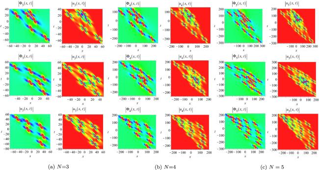
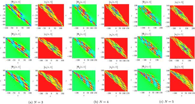
where $({\hat{{\rm{\Phi }}}}_{1}(x,t),{u}_{1}(x,t))$ are the fundamental rogue waves in equation (6), with their positions $({\check{x}}_{0}^{(k)},{\check{t}}_{0}^{(k)})$ given by equation (11). Now we show these predicted rogue wave patterns in figures 4 and 5 and compare them with true rogue wave patterns obtained in section 3. Here, the same α and p0 as those for true rogue waves are selected, all parameters satisfy equation (10) with A = 3. In these panels, the rogue wave patterns are determined by the root structure of the Adler-Moser polynomials through translation, dilation, stretch, rotation and shear. For instance, the third row in figure 4 show the fan-shaped structures.
Figure 4. Predicted NLS-Boussinesq rogue wave patterns when 3 ≤ N ≤ 5 and α = 0. (κ1, κ2, κ3, κ4) are taken as (1, 1, 1, 1), (i, i, i, i) and $\left(\frac{5{\rm{i}}}{3},-{\rm{i}},\frac{5{\rm{i}}}{7},-\frac{5{\rm{i}}}{9}\right)$ in the first, second and third row respectively.
Figure 5. Predicted NLS-Boussinesq rogue wave patterns when 3 ≤ N ≤ 5 and $\alpha =\frac{1}{2}.\left({\kappa }_{1},{\kappa }_{2},{\kappa }_{3},{\kappa }_{4}\right)$ are taken as (1, 1, 1, 1), (i, i, i, i) and $\left(\frac{5{\rm{i}}}{3},-{\rm{i}},\frac{5{\rm{i}}}{7},-\frac{5{\rm{i}}}{9}\right)$ in the first, second and third row respectively.
Now, taking N = 3 as an example, we compare the predicted rogue wave patterns with true ones. Under the same parameters, when α = 0, the true patterns are shown in figures 3(a)-(c), and the prediction patterns are displayed in figure 4(a); when $\alpha =\frac{1}{2}$, the true patterns are illustrated in figures 3(d)-(f) and the prediction patterns are exhibited in figure 5(a). It is evident that the true rogue wave patterns are nearly indistinguishable from the predictions in various aspects, including the individual positions of the fundamental rogue waves, the overall shapes formed by these fundamental waves.

5. Conclusion

In this paper, we gave a detailed analysis of the patterns, with interesting geometric structures, of higher-order rogue wave solutions, depending on multiple parameters, for the NLS-Boussinesq system. For the unique large parameter, rogue wave patterns appear in triangles, pentagons, or their skewed versions [31]. In case of multiple large parameters, many new patterns, associated with the Adler-Moser polynomials, arise and they form heart-, fan-shaped structures or their skewed versions. These predicted rogue wave patterns have been found to describe the true ones with great accuracy, thus the predicted solutions, rather than the true solutions, could be the better candidate for analyzing the dynamics of the rogue wave solutions for their simpler and quicker calculations, especially in higher-order rogue waves.
Here our predicted rogue wave patterns with multiple large parameters were constructed on the assumption that all roots of the Adler-Moser polynomials are simple. Very recently, for the multiple roots of the Adler-Moser polynomials, rogue wave patterns of the NLS equation were given in [26], leading to the discovery of new rogue wave patterns. It would be interesting to build up the rogue wave patterns of system (1) when the Adler-Moser polynomials have some multiple roots in future.

The authors would like to thank the anonymous reviewers for their helpful comments and suggestions. This work is supported by the National Natural Science Foundation of China (Grant Nos. 11871396, 12271433) and Shaanxi Fundamental Science Research Project for Mathematics and Physics (Grant No. 23JSY036). The first author is also partly supported by Graduate Student Innovation Project of Northwest University (Grant No. CX2024129).

1
Akhmediev N, Ankiewicz A, Taki M 2009 Waves that appear from nowhere and disappear without a trace Phys. Lett. A 373 675 678

DOI

2
Peregrine D H 1983 Water waves, nonlinear Schrödinger equations and their solutions J. Austral. Math. Soc. Ser. B 25 16 43

DOI

3
Guo B L, Ling L M, Liu Q P 2012 Nonlinear Schrödinger equation: generalized darboux transformation and rogue wave solutions Phys. Rev. E 85 026607

DOI

4
Ohta Y, Yang J K 2012 General high-order rogue waves and their dynamics in the nonlinear Schrödinger equation Proc. R. Soc. London, Ser. A 468 1716 1740

DOI

5
Ling L M, Guo B L, Zhao L C 2014 High-order rogue waves in vector nonlinear Schrödinger equations Phys. Rev. E 89 041201(R)

DOI

6
Zhao L C, Guo B L, Ling L M 2016 High-order rogue wave solutions for the coupled nonlinear Schrödinger equations-II J. Math. Phys. 57 043508

DOI

7
Ohta Y, Wang D S, Yang J K 2011 General N-dark-dark solitons in the coupled nonlinear Schrödinger equations Stud. Appl. Math. 127 345 371

DOI

8
Zhang X, Wang Y F, Yang S X 2024 Hybrid structures of the rogue waves and breather-like waves for the higher-order coupled nonlinear Schrödinger equations Chaos Solitons Fractals 180 114563

DOI

9
Chen S H, Mihalache D 2015 Vector rogue waves in the Manakov system: diversity and compossibility J. Phys. A 48 215202

DOI

10
Yang B, Yang J K 2021 Universal rogue wave patterns associated with the Yablonskii-Vorob’ev polynomial hierarchy Physica D 425 132958

DOI

11
Li B Q, Ma Y L 2022 Interaction properties between rogue wave and breathers to the Manakov system arising from stationary self-focusing electromagnetic systems Chaos Solitons Fractals 156 111832

DOI

12
Ohta Y, Yang J K 2012 Rogue waves in the Davey-Stewartson I equation Phys. Rev. E 86 036604

DOI

13
Ohta Y, Yang J K 2013 Dynamics of rogue waves in the Davey-Stewartson II equation J. Phys. A 46 105202

DOI

14
Yang B, Yang J K 2021 Rogue wave patterns in the nonlinear Schrödinger equation Physica D 419 132850

DOI

15
Yang B, Yang J K 2020 General rogue waves in the Boussinesq equation J. Phys. Soc. Jpn. 89 024003

DOI

16
Yang B, Yang J K 2021 General rogue waves in the three-wave resonant interaction systems IMA J. Appl. Math. 86 378 425

DOI

17
Zhang X E, Chen Y 2018 General high-order rogue waves to nonlinear Schrödinger-Boussinesq equation with the dynamical analysis Nonlinear Dyn. 93 2169 2184

DOI

18
Kedziora D J, Ankiewicz A, Akhmediev N 2011 Circular rogue wave clusters Phys. Rev. E 84 056611

DOI

19
Kedziora D J, Ankiewicz A, Akhmediev N 2013 Classifying the hierarchy of nonlinear-Schrödinger-equation rogue-wave solutions Phys. Rev. E 88 013207

DOI

20
Ling L M, Zhao L C 2013 Simple determinant representation for rogue waves of the nonlinear Schrödinger equation Phys. Rev. E 88 043201

DOI

21
Zhang Y S, Guo L J, Xu S W, Wu Z Y, He J S 2014 The hierarchy of higher order solutions of the derivative nonlinear Schrödinger equation Commun. Nonlinear Sci. Numer. Simul. 19 1706 1722

DOI

22
Yang B, Yang J K 2022 Pattern transformation in higher-order lumps of the Kadomtsev-Petviashvili I equation J. Nonlinear Sci. 32 52

DOI

23
Dong J Y, Ling L M, Zhang X E 2022 Kadomtsev-Petviashvili equation: one-constraint method and lump pattern Physica D 432 133152

DOI

24
Yang B, Yang J K 2024 Rogue wave patterns associated with Adler-Moser polynomials in the nonlinear Schrödinger equation Appl. Math. Lett. 148 108871

DOI

25
Duan Z Y, Tao X Y, Yang B 2024 Patterns of rogue waves in the sharp-line Maxwell-Bloch system Chaos Solitons Fractals 187 115407

DOI

26
Lin H A, Ling L M 2025 Rogue wave patterns associated with Adler-Moser polynomials featuring multiple roots in the nonlinear Schrödinger equation Stud. Appl. Math. 154 e12782

DOI

27
Rao N N 1989 Exact solutions of coupled scalar field equations J. Phys. A 22 4813

DOI

28
Chowdhury A R, Dasgupta B, Rao N N 1998 Painlevé analysis and Backlund transformations for coupled generalized Schrödinger-Boussinesq system Chaos Solitons Fractals 9 1747 1753

DOI

29
Hase Y, Satsuma J 1988 An N-soliton solution for the nonlinear Schrödinger equation coupled to the Boussinesq equation J. Phys. Soc. Jpn. 57 679 682

DOI

30
Mu G, Qin Z Y 2012 Rogue waves for the coupled Schrödinger-Boussinesq equation and the coupled Higgs equation J. Phys. Soc. Jpn. 81 084001

DOI

31
Fang Q, Duan Z Y, Yang B 2025 Pattern dynamics of higher-order rogue waves in the nonlinear Schrödinger-Boussinesq equation Nonlinear Dyn. 113 3735 3752

DOI

32
Hirota R 1980 Direct Methods in Soliton Theory Springer

33
Adler M, Moser J 1978 On a class of polynomials connected with the Korteweg-de Vries equation Commun. Math. Phys. 61 1 30

DOI

34
Clarkson P A 2009 Vortices and polynomials Stud. Appl. Math. 123 37 62

DOI

Outlines

/