Welcome to visit Communications in Theoretical Physics,
Mathematical Physics

Analyzing point liquid loading effects on transversely isotropic poroelastic media using Green’s function

  • Muzammal Hameed Tariq 1 ,
  • Yue-Ting Zhou , 1, 2
Expand
  • 1 School of Aerospace Engineering and Applied Mechanics, Tongji University, Shanghai 200092, China
  • 2 Shanghai Institute of Aircraft Mechanics and Control, 100 Zhangwu Road, Shanghai 200092, China

Received date: 2024-09-16

  Revised date: 2025-02-08

  Accepted date: 2025-02-10

  Online published: 2025-04-14

Copyright

© 2025 Institute of Theoretical Physics CAS, Chinese Physical Society and IOP Publishing. All rights, including for text and data mining, AI training, and similar technologies, are reserved.
This article is available under the terms of the IOP-Standard License.

Abstract

Understanding the effects of point liquid loading on transversely isotropic poroelastic media is crucial for advancing geomechanics and biomechanics, where precise modeling of fluid-structure interactions is essential. This paper presents a comprehensive analysis of infinite transversely isotropic poroelasticity under a fluid source, based on Biot’s theory, aiming to uncover new and previously unexplored insights in the literature. We begin our study by deriving a general solution for fluid-saturated, transversely isotropic poroelastic materials in terms of harmonic functions that satisfy sixth-order homogeneous partial differential equations, using potential theory and Almansi’s theorem. Based on these general solutions and potential functions, we construct a Green’s function for a point fluid source, introducing three new harmonic functions with undetermined constants. These constants are determined by enforcing continuity and equilibrium conditions. Substituting these into the general solution yields fundamental solutions for poroelasticity that provide crucial support for a wide range of project problems. Numerical results and comparisons with existing literature are provided to illustrate physical mechanisms through contour plots. Our observations reveal that all components tend to zero in the far field and become singular at the concentrated source. Additionally, the contours exhibit rapid changes near the point fluid source but display gradual variations at a distance from it. These findings highlight the intricate behavior of the system under point liquid loading, offering valuable insights for further research and practical applications.

Cite this article

Muzammal Hameed Tariq , Yue-Ting Zhou . Analyzing point liquid loading effects on transversely isotropic poroelastic media using Green’s function[J]. Communications in Theoretical Physics, 2025 , 77(8) : 085001 . DOI: 10.1088/1572-9494/adb415

1. Introduction

Porous materials are intricate entities ubiquitous in natural environments, ranging from the Earth’s soils and rocks to the intricate architecture of living organisms such as plants and human bones [1]. They also extend to synthetic constructs like nano-filtration filters and polyurethane foams. These materials harbor an intricate network of pores or voids, occupying spaces within cavities, fissures, capillary channels, and fractures, dispersed throughout their structure. The distribution of these pores varies in form and size, exhibiting a random orientation and spread [2, 3]. Describing the precise geometry and location of these pores for modeling purposes often proves challenging. Consequently, researchers resort to considering only averaged or homogenized material properties and mechanical responses. Despite the diverse origins of porous materials, their mechanical behaviors are governed by common underlying principles, as elucidated by Verruijt [4].

1.1. Literature survey

The understanding of porous materials advanced significantly with Biot’s poroelasticity theory, which explored phase interactions in poroelastic solids [5]. Subsequent contributions spanned various disciplines, enhancing the field’s scope. Takizawa et al [6] accurately modeled geometric porosity in spacecraft-parachute designs using the space-time method, introducing ST computational methods for compressible-flow aerodynamics. Wang et al [7] integrated machine learning with classical constitutive laws to model multiscale hydro-mechanical coupling in multi-porosity porous media, improving computational efficiency and robustness. Sahebkar et al [8] applied the (u − p) formulation of Biot’s equations to analyze mechanical and hydraulic dynamics under time-harmonic fluid ring flux and vertical circular loads, employing Fourier and Hankel transforms. Carcione et al [9] used a time-fractional diffusion equation and staggered Fourier pseudospectral method to simulate fluid flow in anisotropic porous media, capturing memory effects and anomalous diffusion. Le Bars & Worster [10] enhance the consistency between single-domain and multiple-domain models for fluid flow through porous and fluid regions by introducing a viscous transition zone, ensuring continuity of pressure and velocities, which leads to more accurate predictions of solidification patterns. Ba et al [11] examined the 3D dynamic responses of multi-layered poroelastic media using Fourier expansion, Hankel transform, and the direct stiffness method. Kulawiak et al [12] developed a poroelastic two-phase model to analyze the self-organized droplet motion, validated by numerical simulations that reproduce experimental oscillatory behaviors and flow patterns. Additionally, investigations into heat transfer and fluid flow in porous media have extensively examined various phenomena, including Magnetohydrodynamic natural convection, viscoelastic fluid flow, and hybrid nanofluid convection, utilizing diverse numerical methods. These studies have significantly contributed to advancing the understanding of the complex interactions in porous media [1317]. Other than that, solids and rocks are seldom isotropic due to the geological processes of sedimentation. However, limited research has been conducted on the behavior of anisotropic media under fluid loads [18]. The interaction between the solid phase and the interpenetrating fluids in the porous medium results in fluid flow, which in turn causes solid deformation. Therefore, it is crucial to examine the impact of the fluid source on anisotropic porous formations. However, obtaining an analytical solution for the anisotropic poroelasticity model is challenging due to the complexity of the solid stress and fluid pressure fields.
The Green’s functions of poroelastic materials are crucial in both applied and theoretical studies, including in hydrology [19, 20]. Therefore, Green’s function is employed to solve the boundary value problem for point liquid loading on transversely isotropic saturated poroelastic media, owing to its ability to provide both efficient and accurate solutions. It is particularly valuable in saturated poroelastic systems for capturing interface effects and stress distributions, which are essential for analyzing complex interactions between fluid and solid phases. For instance, in applications like poroelastic water-beds composed of different poroelastic materials, interface effects significantly influence the movement and failure of the system, making precise analysis essential. Green’s function provides a robust framework for analyzing these effects, including soil stress states and addressing hydrologic problems, making it indispensable in such studies. Compared to numerical methods like finite element or finite difference techniques, which require discretization of the entire domain and can become computationally intensive, Green’s function focuses on the boundaries, simplifying the problem and reducing computational complexity. Its analytical nature facilitates the direct incorporation of boundary conditions, making it essential for deriving boundary integral equations used in the boundary element method [2123], thereby enabling more efficient and accurate solutions. Furthermore, its adaptability makes it effective across various domains, from geomechanics and biomechanics to hydrology, seismic analysis, and telecommunications [2427]. These advantages underscore the significance of Green’s function in solving the coupled field problems in this paper, aligning with the study’s objective of advancing understanding in the interaction between point liquid loading and poroelastic media.
In recent decades, researchers have extensively studied Green’s functions for various materials, including anisotropic, orthotropic, isotropic, and two-phase systems, with a focus on the impact of coupling effects. For instance, Li et al [28] delved into three-dimensional (3D) Green’s function solutions for double-layer transversely isotropic thermoelastic plates, shedding light on temperature and thermal-stress fields pivotal for thermal design considerations. Tariq et al [29, 30] ventured into developing 2D and 3D solutions, considering multiple coupling effects for single-point loading of moisture and temperature using Green’s function. Ding et al [31] derived Green’s functions for two-phase transversely isotropic magneto-electro-elastic media using a trial-and-error method, providing exact and explicit solutions useful for boundary element method computations. Jinxi et al [32] crafted novel Green’s functions for an infinite 2D anisotropic magnetoelectroelastic medium with an elliptical cavity, employing advanced mathematical formalisms. Hwu and Chen [33] derived Green’s functions for anisotropic and piezoelectric bimaterials using Stroh’s formalism and analytical continuation, creating a special boundary element method that ensures accurate and efficient interface continuity without meshes. Zhao et al [34] derived a simplified general solution for 3D hygrothermoelastic media under single-point loading. Additionally, Lee and Jiang et al [35, 36] compiled a comprehensive set of Green’s functions for orthotropic materials, covering both infinite media and half spaces using the superposition method. Further, Rajapakse et al [37] examined the 3D response of a poroelastic half-space with a compressible constituent through Fourier expansions and Hankel transforms Kaynia [38], on the other hand, derived Green’s functions for dynamic poroelasticity within the Laplace transform domain. These studies have offered invaluable insights into material behavior within multi-field environments and have found diverse applications across various engineering and scientific domains, such as soil consolidation, bioscience, and filtration [3942].

1.2. Novelty and unique contributions

Although previous studies, including those by Takizawa et al [6], Wang et al [7], Abo-Dahab et al [13], Mebarek-Oudina et al [15], Carcione et al [9], and Le Bars & Worster [10], have explored various aspects of poroelastic materials, our study introduces a pioneering advancement in the field. We derive compact mono-harmonic general solutions through advanced potential theory, specifically tailored for transversely isotropic poroelastic materials with distinct eigenvalues, satisfying sixth-order partial differential equations. Leveraging these solutions, we construct a 2D fundamental solution for fluid-saturated, infinite transversely isotropic poroelastic planes under a steady-state point fluid source. This advancement introduces three innovative harmonic functions, formulated via Green’s function and advanced potential formulations, and elegantly expressed in terms of elementary functions to ensure both simplicity and practical applicability.
To handle complex boundary conditions and coupled multi-field problems, we extend established techniques, including operator theory [43], Almansi’s theorem [44], and extending Fabrikant’s potential theory method from elasticity to poroelasticity [45], alongside Green’s function [21], we derive exact and explicit solutions that facilitate precise computations, particularly in boundary element methods. These techniques simplify complex boundary conditions, enhancing solution accuracy and making them ideal for addressing coupled fields in both 2D and 3D multi-field materials. Their remarkable effectiveness has been demonstrated in various applications, including cracks, punches, and inclusions [4649], further establishing their utility in solving intricate poroelastic problems essential for understanding system behavior under point loading. Moreover, rigorous validation and numerical analysis, with graphical contours, confirm the accuracy and provide insights into pore fluid pressure and stress distributions.
The significance of this work lies in its ability to enhance accuracy and reliability across a range of domains, including engineering [45], geomechanics [50], geothermal studies [25], elasticity theory [48], and fracture mechanics [49]. By addressing key challenges in inverse problems with exact solutions, our study advances predictive and management strategies across these critical domains.
The following strategy is used in the current investigation: the first phase introduces the fundamental constitutive equations within a Cartesian framework. In the second section, we derive the general solutions of the governing model using differential operator theory and the superposition principle. In the third phase, we develop innovative Green’s functions based on these solutions and potential functions, incorporating undetermined constants to represent a fluid source at a specific point. The fourth phase involves determining these unknown constants through equilibrium and continuity conditions. These functions are then synthesized into a comprehensive general solution, resulting in a fully integrated coupled field. Finally, our discussion concludes with a rigorous numerical analysis to evaluate the validity and robustness of the findings, including a comparative analysis with existing literature to affirm the effectiveness of our solution.

2. Problem statement

The problem involves analyzing the behavior of an infinite transversely isotropic fluid-saturated poroelastic plane under the influence of a concentrated fluid source $\tilde{F}$ at the origin of the 2D Cartesian coordinate system. The principal material directions are aligned along the x- and z-axes. The rectangular domain is defined by  − txt(t > 0) and b1zb2. A porous medium is centered within the rectangle, with an applied point force $\tilde{F}$ at the origin, as shown in figure 1. We aim to determine the coupling of mechanical and pore pressure distribution within the medium under the following boundary conditions (BC):

Continuity of displacement w and shear stress σzx on the plane z = 0.

The net resultant of normal stress in the z-direction and and the shear stress in the x-direction is zero across the specified rectangular region.

The net fluid flux across the boundaries of the rectangular region must balance with the applied fluid source $\tilde{F}$.

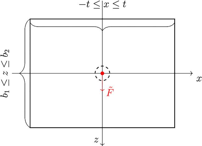
Figure 1. Illustration of the boundary value problem for a transversely isotropic poroelastic material.
Since the problem is considered in a steady-state scenario, initial conditions (IC) are not required for this analysis.

2.1. Basic equations

Basic governing equations of transversely isotropic fluid-saturated poroelastic materials can be found [27, 51] under the assumption that the combined mechanical and fluid pressure loads vary slowly with time and the rate of fluid mass content diminishes. As a result, the poroelastic media are considered to be in a steady-state, with the pore fluid pressure remaining constant over time.

Constitutive Hooke’s law

$\begin{eqnarray}\begin{array}{rcl}{\sigma }_{x} & = & {c}_{11}{\epsilon }_{x}+{c}_{13}{\epsilon }_{z}-{\alpha }_{11}^{* }P,\\ {\sigma }_{z} & = & {c}_{13}{\epsilon }_{x}+{c}_{33}{\epsilon }_{x}-{\alpha }_{33}^{* }P,\\ {\sigma }_{zx} & = & {c}_{44}{\gamma }_{zx}.\end{array}\end{eqnarray}$

Pressure law

$\begin{eqnarray}P=M(\xi -{\alpha }_{11}^{* }{\epsilon }_{x}-{\alpha }_{33}^{* }{\epsilon }_{z}).\end{eqnarray}$

Quasi-Laplace and Balance equations (absence of body forces)

$\begin{eqnarray}{k}_{ij}{P}_{,jj}=0,\,{\sigma }_{ij,j}=0.\end{eqnarray}$

In equations ((1)–(3)), σij where (ij = xz) represent the normal and shear stress components. The strain components are defined as εx = ∂u/∂x, εz = ∂w/∂z, and γzx =∂w/∂x + ∂u/∂z, where u, w, and P denote the mechanical displacement components and pore pressure variations, respectively. The Biot effective stress coefficients are denoted by ${\alpha }_{ij}^{* }$, and the elastic moduli are represented by cij. Additionally, ξ represents a change in fluid content, M represents Biot’s modulus, and kij are coefficients of fluid permeability. The symbol , refers to the partial derivative with respect to spatial coordinates x and z.
It is important to highlight that the elastic moduli cij and the Biot coefficient ${\alpha }_{ij}^{* }$ are connected to the engineering elastic moduli, which provide the link between the theoretical framework and practical engineering applications. These relationships are essential for interpreting the material properties in terms of measurable quantities commonly used in engineering design and analysis. The relationships can be expressed as follows [5153]:
$\begin{eqnarray}\begin{array}{l}{c}_{11}=\displaystyle \frac{E({E}^{{\prime} }-E{\nu {}^{{\prime} }}^{2})}{(1+\nu )({E}^{{\prime} }-{E}^{{\prime} }\nu -2E{\nu {}^{{\prime} }}^{2})},\,{c}_{13}=\displaystyle \frac{E{E}^{{\prime} }{\nu }^{{\prime} }}{{E}^{{\prime} }-{E}^{{\prime} }\nu -2E{\nu {}^{{\prime} }}^{2}},\,\,{c}_{44}={G}^{{\prime} }=\displaystyle \frac{E}{2(1+{\nu }^{{\prime} })},\\ {\alpha }_{11}^{* }=1-\displaystyle \frac{{c}_{11}+{c}_{13}}{3{K}_{s}},\,{\alpha }_{33}^{* }=1-\displaystyle \frac{2{c}_{13}+{c}_{33}}{3{K}_{s}},\,{k}_{11}=\displaystyle \frac{{\kappa }_{1}}{\mu },\,{k}_{33}=\displaystyle \frac{{\kappa }_{3}}{\mu },\end{array}\end{eqnarray}$
where κ1 and κ3 represent the components of the anisotropic permeability tensor, μ denotes the pore fluid viscosity, and Ks refers to the bulk modulus of the solid skeleton. The unprimed parameters E, ν, G, and ${\alpha }_{11}^{}$ denote the drained Young’s modulus, Poisson’s ratio, shear modulus, and Biot’s effective stress coefficient in the isotropic plane of the geomaterial. Conversely, the primed parameters ${E}^{{\prime} }$, ${\nu }^{{\prime} }$, ${G}^{{\prime} }$, and ${\alpha }_{33}^{}$ refer to the corresponding properties in the transverse plane along the axis of rotational symmetry.

3. General solution

In this section, we derive the static general solution for the governing equations. To achieve this, we substitute equation (1) into equation (3), resulting in
$\begin{eqnarray}{ \mathcal D }{[{H}_{1}{H}_{2}{H}_{3}]}^{{\rm{T}}}={[000]}^{{\rm{T}}},\end{eqnarray}$
$\begin{eqnarray}{ \mathcal D }=\left[\begin{array}{ccc}{h}_{11} & {h}_{12} & {h}_{13}\\ {h}_{21} & {h}_{22} & {h}_{23}\\ {h}_{31} & {h}_{32} & {h}_{33}\end{array}\right],\end{eqnarray}$
where ${ \mathcal D }$ represents the matrix operator, hij is defined in the appendix, and Hi = δi1u + δi2w + δi3P, where δij(ij = 1, 2, 3) is the Kronecker delta defined as δij = 1 for i = j and δij = 0 for i ≠ j. Further, the determinant of ${ \mathcal D }$ can be computed as follows:
$\begin{eqnarray}\begin{array}{rcl}| { \mathcal D }| & = & \left(a\displaystyle \frac{{\partial }^{4}}{\partial {z}^{4}}+b\displaystyle \frac{{\partial }^{4}}{\partial {x}^{2}\partial {z}^{2}}+c\displaystyle \frac{{\partial }^{4}}{\partial {x}^{4}}\right)\\ & & \times \left({k}_{11}\displaystyle \frac{{\partial }^{2}}{\partial {x}^{2}}+{k}_{33}\displaystyle \frac{{\partial }^{2}}{\partial {z}^{2}}\right),\end{array}\end{eqnarray}$
where $a={c}_{33}{c}_{44},\,b={c}_{33}{c}_{11}+{c}_{44}^{2}-{({c}_{13}+{c}_{44})}^{2}$, and c =c11c44. Using operator theory [43] the general solution of equation (5) can be stated as:
$\begin{eqnarray}{H}_{i}=({\delta }_{i1}{{ \mathcal D }}_{k1}+{\delta }_{i2}{{ \mathcal D }}_{k2}+{\delta }_{i3}{{ \mathcal D }}_{k3})F\,\,(i=1,2,3),\end{eqnarray}$
where ${{ \mathcal D }}_{kj}$ with kj = 1, 2, 3 represent a cofactor of ${ \mathcal D }$, and function F satisfy the following equations:
$\begin{eqnarray}| { \mathcal D }| F=0.\,\end{eqnarray}$
The solution to equation (9) is denoted by F, which can be expressed as follows:
$\begin{eqnarray}\displaystyle \prod _{j=1}^{3}\left(\frac{{\partial }^{2}}{\partial {x}^{2}}+\frac{{\partial }^{2}}{\partial {z}_{j}^{2}}\right)F=0,\end{eqnarray}$
where zj = sjz, ${s}_{3}=\sqrt{{k}_{11}/{k}_{33}}$, and sj for j = 1, 2 denote the two positive real roots of the following equation:
$\begin{eqnarray}a{s}^{4}-b{s}^{2}+c=0.\end{eqnarray}$
Now, deriving the solution of equation (8) for k = 3 and reformulating the solution of equation (10) using the generalized Almansi’s theorem [44] (F = F1 + F2 + F3) for distinct sj, we have
$\begin{eqnarray}\begin{array}{rcl}{H}_{i} & = & \displaystyle \sum _{j=1}^{3}\left[{\delta }_{i1}\left({Q}_{1j}\frac{{\partial }^{3}{F}_{j}}{\partial x\partial {z}_{j}^{2}}\right)\right.\\ & & \left.+{\delta }_{i2}\left({Q}_{2j}{s}_{j}\frac{{\partial }^{3}{F}_{j}}{\partial {z}_{j}^{3}}\right)+{\delta }_{i3}\left({Q}_{3j}\frac{{\partial }^{4}{F}_{j}}{\partial {z}_{j}^{4}}\right)\right],\end{array}\end{eqnarray}$
where
$\begin{eqnarray}\left(\frac{{\partial }^{2}}{\partial {x}^{2}}+\frac{{\partial }^{2}}{\partial {z}_{j}^{2}}\right){F}_{j}=0\,\,(j=1,2,3),\end{eqnarray}$
$\begin{eqnarray}\begin{array}{rcl}{Q}_{kj} & = & -{a}_{k}+{b}_{k}{s}_{j}^{2}\,\,(k=1,2),\\ {Q}_{31} & = & {Q}_{32}=0,\,{Q}_{33}=a{s}_{3}^{4}-b{s}_{3}^{2}+c.\end{array}\end{eqnarray}$
Utilizing symbolic computation tools, the values of ak and bk can be determined. Additionally, assuming
$\begin{eqnarray}{Q}_{1j}\frac{{\partial }^{2}{F}_{j}}{\partial {z}_{j}^{2}}={\psi }_{j}\,\,(j=1,2,3).\end{eqnarray}$
Using equations (14), (12) has been further clarified,
$\begin{eqnarray}{H}_{i}=\displaystyle \sum _{j=1}^{3}\left[{\delta }_{i1}\left(\frac{\partial {\psi }_{j}}{\partial x}\right)+{\delta }_{i2}\left({M}_{1j}{s}_{j}\frac{\partial {\psi }_{j}}{\partial {z}_{j}}\right)+{\delta }_{i3}\left({M}_{2j}\frac{{\partial }^{2}{\psi }_{j}}{\partial {z}_{j}^{2}}\right)\right],\end{eqnarray}$
where M1j = Q2j/Q1j, M21 = M22 = 0, and M23 = Q33/Q13. This can be observed from equations (13a) and (14) that the functions ψj in equation (15) continue to satisfy the following equation:
$\begin{eqnarray}\left(\frac{{\partial }^{2}}{\partial {x}^{2}}+\frac{{\partial }^{2}}{\partial {z}_{j}^{2}}\right){\psi }_{j}=0\,\,(j=1,2,3).\end{eqnarray}$
Substituting equation (15) into equation (1) and subsequently simplifying with the aid of equation (3) and equation (16), we have
$\begin{eqnarray}\begin{array}{rcl}{H}_{i}^{* } & = & \displaystyle \sum _{j=1}^{3}{N}_{j}\left[-{\delta }_{i1}\left({s}_{j}^{2}\displaystyle \frac{{\partial }^{2}{\psi }_{j}}{\partial {z}_{j}^{2}}\right)\right.\\ & & +\,\left.{\delta }_{i2}\left(\displaystyle \frac{{\partial }^{2}{\psi }_{j}}{\partial {z}_{j}^{2}}\right)+{\delta }_{i3}({s}_{j}\displaystyle \frac{{\partial }^{2}{\psi }_{j}}{\partial x\partial {z}_{j}})\right],\end{array}\end{eqnarray}$
where
$\begin{eqnarray*}\begin{array}{rcl}{H}_{i}^{* } & = & {\delta }_{i1}{\sigma }_{x}+{\delta }_{i2}{\sigma }_{z}+{\delta }_{i3}{\sigma }_{zx}\,(i=1,2,3),\\ {N}_{j} & = & [{c}_{11}-{c}_{13}{M}_{1j}{s}_{j}^{2}+{M}_{2j}{\alpha }_{11}^{* }]/{s}_{j}^{2}\\ & = & [{c}_{44}(1+{M}_{1j})]\\ & = & [-{c}_{13}+{M}_{1j}{c}_{33}{s}_{j}^{2}-{M}_{2j}{\alpha }_{33}^{* }].\end{array}\end{eqnarray*}$
In the subsequent section, we employ the obtained general solution (equation (15) and (17)).

4. Green’s function

In this example, we consider an infinite transversely isotropic poroelastic plane with principal material directions aligned along the x- and z-axes. We apply a concentrated fluid source $(\tilde{F})$ at the origin of the 2D Cartesian coordinate system (x, z) (figure 1). By using general solutions provided in equations(15) and (17), we derive the coupled field in this infinite poroelastic plane. Furthermore, we introduce potential functions [54, 55] below that satisfy the Laplace equation (16) and meet our boundary conditions:
$\begin{eqnarray}{\psi }_{j}={{\rm{\Xi }}}_{j}\mathrm{ln}({R}_{j}^{* }),\end{eqnarray}$
where j = 1, 2, 3 and ${R}_{j}^{* }=\sqrt{{x}^{2}+{z}_{j}^{2}}$. The three unknown constants are denoted by Ξj. After substituting equation (18) into equation (17) and (15), we have
$\begin{eqnarray}\begin{array}{rcl}{H}_{i} & = & \displaystyle \sum _{j=1}^{3}\displaystyle \frac{{{\rm{\Xi }}}_{j}}{{R}_{j}^{* 2}}\left[{\delta }_{i1}x+{\delta }_{i2}({M}_{Ij}{s}_{j}{z}_{j})\right.\\ & & \left.+{\delta }_{i3}{M}_{2j}\left(\displaystyle \frac{({x}^{2}-{z}_{j}^{2})}{{R}_{j}^{* 2}}\right)\right],\\ {H}_{i}^{* } & = & \displaystyle \sum _{j=1}^{3}\displaystyle \frac{{{\rm{\Xi }}}_{j}{N}_{j}}{{R}_{j}^{* 4}}\left[({x}^{2}-{z}_{j}^{2}){\delta }_{i2}-{s}_{j}^{2}{\delta }_{i1}-2x{s}_{j}{z}_{j}{\delta }_{i3}\right]\\ & & \,(i=1,2,3).\end{array}\end{eqnarray}$
Considering the continuous conditions on the plane z = 0 for w and σzx yields
$\begin{eqnarray}\displaystyle \sum _{j=1}^{3}{\varpi }_{i}({{\rm{\Xi }}}_{j})=0\,\,(i=1,2),\end{eqnarray}$
where ϖi = δi1M1jsj + δi2Njsj. Putting the value of Nj in equation (20), we have
$\begin{eqnarray}\displaystyle \sum _{j=1}^{3}{\varpi }_{i}^{* }({{\rm{\Xi }}}_{j})=0,\end{eqnarray}$
where ${\varpi }_{i}^{* }={\delta }_{i1}{M}_{1j}{s}_{j}+{\delta }_{i2}{s}_{j}$. Moreover, when we consider mechanical and pressure equilibrium for the rectangle with b1 ≤ z ≤ b2 (b1 < 0 < b2) and  − t ≤ x ≤ t (t > 0), it results in two additional equations: one for the resultant force and the other for fluid mass content, we have
$\begin{eqnarray}{\left.{\int }_{-t}^{t}{\sigma }_{z}(x,z)\right|}_{z={b}_{1}}^{z={b}_{2}}\,{\rm{d}}x{\left.+{\int }_{{b}_{1}}^{{b}_{2}}{\sigma }_{zx}(x,z)\right|}_{x=-t}^{x=t}\,{\rm{d}}z=0,\end{eqnarray}$
$\begin{eqnarray}\begin{array}{l}{\left.-{k}_{33}{\displaystyle \int }_{-t}^{t}\displaystyle \frac{\partial P}{\partial z}(x,z)\right|}_{z={b}_{1}}^{z={b}_{2}}\,{\rm{d}}x\\ {\left.-{k}_{11}{\displaystyle \int }_{{b}_{1}}^{{b}_{2}}\displaystyle \frac{\partial P}{\partial x}(x,z)\right|}_{x=-t}^{x=t}\,{\rm{d}}z=\tilde{F},\end{array}\end{eqnarray}$
where the permeability coefficients are denoted as k11 and k33, substituting equation (19) into equations (22a) and (22b), using ${s}_{3}=\sqrt{{k}_{11}/{k}_{33}}$, we have
$\begin{eqnarray}\displaystyle \sum _{j=1}^{3}{{\rm{\Xi }}}_{j}{N}_{j}{I}_{1}=0,\end{eqnarray}$
$\begin{eqnarray}{{\rm{\Xi }}}_{3}{I}_{2}=-\displaystyle \frac{\tilde{F}}{{M}_{23}\sqrt{{k}_{11}{k}_{33}}},\end{eqnarray}$
where
$\begin{eqnarray}\begin{array}{rcl}{I}_{1} & = & {\left[x\left(\displaystyle \frac{1}{{R}_{j}^{* 2}(x,{b}_{1})}-\displaystyle \frac{1}{{R}_{j}^{* 2}(x,{b}_{2})}\right)\right]}_{x=-t}^{x=t}\\ & & +{\left[\displaystyle \frac{2t}{{R}_{j}^{* 2}(x,z)}\right]}_{z={b}_{1}}^{z={b}_{2}}=0,\end{array}\end{eqnarray}$
$\begin{eqnarray}\begin{array}{rcl}{I}_{2} & = & {\left[2{s}_{3}x\left(\displaystyle \frac{{b}_{2}}{{R}_{j}^{* 2}(x,{b}_{2})}-\displaystyle \frac{{b}_{1}}{{R}_{j}^{* 2}(x,{b}_{1})}\right)\right]}_{x=-t}^{x=t}\\ & & -{\left[\displaystyle \frac{4t{z}_{i}}{{R}_{j}^{* 2}(t,z)}\right]}_{z={b}_{1}}^{z={0}^{-}}-{\left[\displaystyle \frac{4t{z}_{i}}{{R}_{j}^{* 2}(t,z)}\right]}_{z={0}^{+}}^{z={b}_{2}}.\end{array}\end{eqnarray}$
As a result, equations (22a) and (23) are automatically satisfied, while Ξ3 can be determined by equations (26) and (24), we have
$\begin{eqnarray}{{\rm{\Xi }}}_{3}=\frac{\tilde{F}}{7{M}_{23}\sqrt{{k}_{11}{k}_{33}}}.\end{eqnarray}$
Moreover, Ξj for j = 1, 2 can be determined from equation (21) as follows:
$\begin{eqnarray}\begin{array}{rcl}{{\rm{\Xi }}}_{j} & = & \displaystyle \frac{{{\rm{\Xi }}}_{3}{s}_{3}}{{M}_{11}-{M}_{12}}\left[{\delta }_{j1}({M}_{12}-{M}_{13})/{s}_{1}\right.\\ & & \left.+{\delta }_{j2}({M}_{13}-{M}_{11})/{s}_{2}\right].\end{array}\end{eqnarray}$
After thorough analysis and calculations, the comprehensive solution for the infinite transversely isotropic poroelastic field, responding to a point fluid source, has been successfully derived (equation (19)). The depth and complexity of this solution offer valuable insights into the intricate mechanics governing poroelastic behavior within anisotropic materials.

5. Numerical results and discussion

In this section, we explore the numerical results concerning infinitely transversely isotropic poroelastic materials and compare our findings with those presented in the existing literature. Furthermore, the numerical calculations are based on the material properties provided in [5658], which are listed in table 1.
Table 1. The material properties of poroelastic media [5658].
Material property Materials
Elastic constants (×109N/m2) c11 74.1 c33 83.6
c13 39.3 c44 13.2

Intrinsic permeability (darcy = 10−12 m2) κ1 0.5 κ3 0.1

Bulk modulus of solid skeleton(GPa) Ks 37.9

Fluid viscosity (cp) μ 0.024
Additionally, we used the following equations to determine the remaining physical parameters and non-dimensional components as follows:
$\begin{eqnarray}\begin{array}{rcl}\zeta & = & \displaystyle \frac{x}{{x}_{0}},\,\chi =\displaystyle \frac{z}{{x}_{0}},\,\bar{P}=\displaystyle \frac{P}{{c}_{ij}},\\ {{u}}_{k} & = & \displaystyle \frac{{{u}}_{i}}{{x}_{0}},\,{\sigma }_{k}=\displaystyle \frac{{\sigma }_{i}}{{c}_{ij}},\\ {\sigma }_{kl} & = & \displaystyle \frac{{\sigma }_{ij}}{{c}_{ij}}\,(i,j=x,z;k,l=\zeta ,\chi ),\\ {k}_{11} & = & \displaystyle \frac{{\kappa }_{1}}{\mu },\,\,{k}_{33}=\displaystyle \frac{{\kappa }_{3}}{\mu },\,\,{\alpha }_{11}^{* }=1-\displaystyle \frac{{c}_{11}+{c}_{13}}{3{K}_{s}},\\ {\alpha }_{33}^{* } & = & 1-\displaystyle \frac{2{c}_{13}+{c}_{33}}{3{K}_{s}},\end{array}\end{eqnarray}$
where ${x}_{0}=\left|{b}_{2}-{b}_{1}\right|$ is a characteristic length scale, which is a non-zero constant.

5.1. Verification of the derived solutions

To validate the derived solutions, we follow a two-step approach. First, we compare the results for the purely elastic case with those from published studies. Second, we verify the solutions by substituting them into the original governing equations.
For the purely elastic case, we eliminate the pressure loading by setting kij = 0 and ${\alpha }_{ij}^{* }=0$. Under these conditions, the non-dimensional displacement and stress components are expressed as:
$\begin{eqnarray}{u}_{\zeta }=\displaystyle \sum _{j=1}^{2}\left[\frac{\partial {\psi }_{j}}{\partial x}\right],\quad {\sigma }_{\chi }=\displaystyle \sum _{j=1}^{2}\left[{N}_{j}\frac{{\partial }^{2}{\psi }_{j}}{\partial {z}_{j}^{2}}\right].\end{eqnarray}$
These results align with those presented by Hou et al [59] in equations (16) and (12) after excluding the thermal modules and heat conduction coefficients. Similarly, setting y = 0 and φ3 = 0 in the equations (2.256) and (2.263) from Ding et al [54] yields comparable results, as shown in equation (30). Thus, both solutions represent purely elastic behavior, unaffected by pressure or temperature effects.
To further validate the results, we compare the non-dimensional displacement (uζ) and stress (σχ) components with Hou et al [59] at χ = 1, using equation (22a) and the material properties listed in table 1. This comparison is illustrated in Figures 2 and 3, where the solid line represents the solution from [59], and the dots depict the present solution (PS). The strong agreement between the two solutions confirms the validity of the current work.
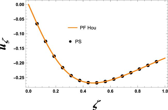
Figure 2. Comparison of the dimensionless displacement component uζ × 1012 with PF Hou at χ = 1.
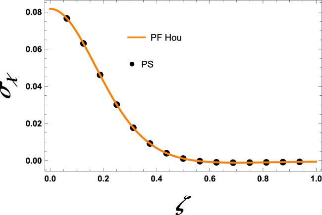
Figure 3. Comparison of the dimensionless normal stress component σχ × 1011 with PF Hou at χ = 1.
To verify the derived expression for pore water pressure, we substitute the final result of pore pressure into the Quasi-Laplace equation (3). The derived expression for pore pressure can be written as:
$\begin{eqnarray}P=\frac{{M}_{23}{{\rm{\Xi }}}_{3}}{{R}_{3}^{* 4}}({x}^{2}-{z}_{3}^{2}),\end{eqnarray}$
where M23, ${R}_{3}^{* }$, and Ξ3 are defined in equations (15), (18), and (27), respectively. Additionally, z3 = s3z, with ${s}_{3}=\sqrt{{k}_{11}/{k}_{33}}$, and kij representing the coefficients of fluid permeability.
Substituting equation (31) into the Quasi-Laplace equation (equation (3)), and simplifying using z3 = s3z and ${s}_{3}=\sqrt{{k}_{11}/{k}_{33}}$, we have
$\begin{eqnarray}\begin{array}{l}\left({k}_{11}\frac{{\partial }^{2}}{\partial {x}^{2}}+{k}_{33}\frac{{\partial }^{2}}{\partial {z}^{2}}\right)\\ \,=\,\frac{6{M}_{23}{{\rm{\Xi }}}_{3}({x}^{4}-6{x}^{2}{z}^{2}{s}_{3}^{2}+{z}^{4}{s}_{3}^{4})}{{R}_{3}^{* 8}}\left[{k}_{11}-{k}_{33}{s}_{3}^{2}\right]\\ \,=\,\frac{6{M}_{23}{{\rm{\Xi }}}_{3}({x}^{4}-6{x}^{2}{z}^{2}{s}_{3}^{2}+{z}^{4}{s}_{3}^{4})}{{R}_{3}^{* 8}}\left[{k}_{11}-{k}_{11}\right]\\ \,P\,=\,0.\end{array}\end{eqnarray}$
This result demonstrates that the solution satisfies both the original governing equations and the associated boundary conditions, thereby validating the derived solutions.

5.2. Examining poroelastic component contours with under point fluid source

The non-dimensional contour behaviors of pore fluid pressure, displacement, and stress components induced by the liquid source $(\tilde{F}=1.0\,{\rm{kg}}\,{{\rm{s}}}^{-1})$ at the origin are depicted in figures 47. Other physical descriptions of the figures are provided below:
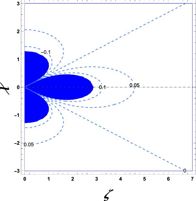
Figure 4. Contour behavior of dimensionless poro fluid pressure $\bar{P}\times 1{0}^{2}$ under point liquid source.
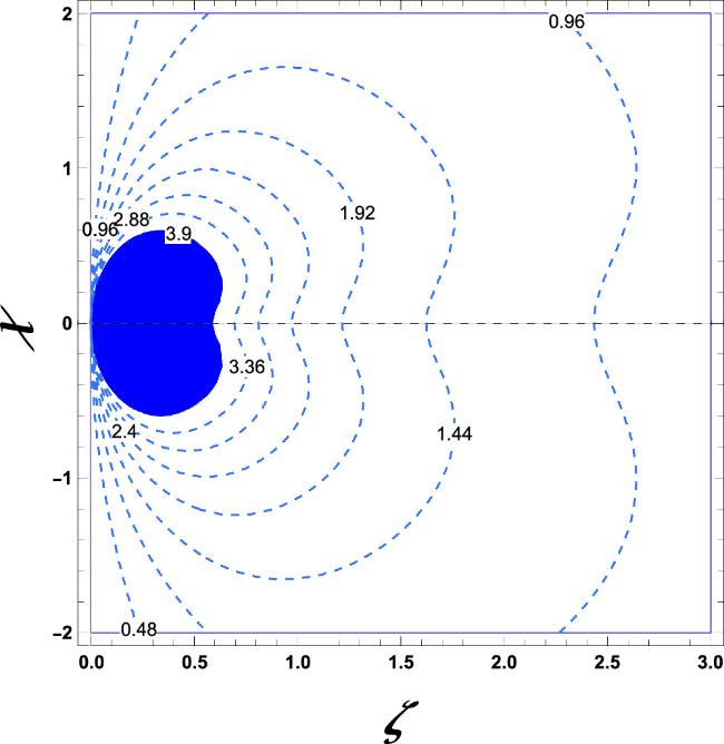
Figure 5. Contour behavior of dimensionless displacement uζ × 10−7 under point liquid source.
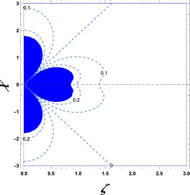
Figure 6. Contour behavior of dimensionless normal stress σχ × 10−8 under point liquid source.
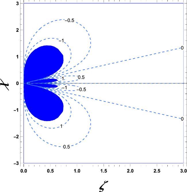
Figure 7. Contour behavior of dimensionless shear stress σχζ × 10−7 under point liquid source.
In figure 4, we observe the non-dimensional contours of pore pressure for transversely isotropic materials. The contours show dense and abrupt variation near the concentrated source, gradually changing as distance increases. Furthermore, it is worth noting that these contours exhibit an almost elliptical behavior, particularly around the high-pressure regions near the origin. This can be attributed to the varying permeability coefficients of fluids such as k11 and k33. Moreover, we observed that the fluid flow, driven by the pressure gradient, indeed moves perpendicular to the contour lines from high-pressure regions toward low-pressure regions. This behavior is consistent with the principles of fluid flow in porous media, illustrating the directional flow dynamics within the poroelastic material.
The behavior of the non-dimensional contours of the displacement component (u or uζ) in a poroelastic transversely isotropic material is illustrated in figure 5. We observed that, the contour lines exhibit a positive trend, and show higher displacement values near the origin due to a fluid source, gradually decreasing with distance. The dense clustering of contours near high-displacement regions indicates a steep gradient, reflecting significant deformation from applied loads or fluid interactions. This highlights the importance of considering anisotropy and poroelastic coupling in material analysis.
In figure 6, the distribution of normal stress (σz or σζ) induced by a point liquid source within an infinitely extended transversely isotropic poroelastic material is illustrated. The contours exhibit a symmetrical heart-like pattern about the ζ-axis, particularly near regions of higher stress values (e.g., 0.2), highlighting the anisotropic nature of the material. Additionally, points of inflection and a zero common tangent are observed. Further, the contours undergo rapid changes in close proximity to the concentrated source, while displaying more gradual variations as one moves farther away from it. These features emphasize the importance of anisotropy and poroelastic coupling in determining the stress distribution and mechanical behavior under steady-state conditions.
In figure 7, we present non-dimensional contours illustrating shear stress (σzx or σχζ) beneath the point liquid source. Our observations reveal the presence of multiple zero common tangents along the ζ-axis for shear stress, with positive values observed below some tangents and negative values above, while for others, negative values are above and positive values are below. Importantly, a higher-order singularity is identified at the liquid source, where the tangents converge into a single tangent. This unique configuration suggests the possibility of shear failure in the material.
Furthermore, in the depicted contours, it is observed that all components tend to zero in the far field and become singular at the concentrated source. Additionally, the contours show rapid changes in the vicinity of the point source but display gradual variations at a distance from it. This complexity poses challenges for numerical simulations, especially when employing methods like finite element analysis, which require very fine meshes to accurately capture such intricate behavior.

6. Conclusion

In this study, we focused on analyzing the effects of point liquid loading on transversely isotropic saturated poroelastic media, a key challenge in fluid-structure interactions. By utilizing potential theory and Green’s function, we derived a general solution that incorporates poroelastic coupling and developed a fundamental solution for fluid-saturated, infinite transversely isotropic poroelastic media under a steady-state point fluid source. This explicit and robust framework offers reliable, exact solutions, making it highly applicable for computation with boundary element methods [2123]. Furthermore, we rigorously validated the solution and presented detailed numerical examples, with the analysis performed using contour plots. The insights gained from these analyses are summarized as key findings below:

The pore pressure contours display dense, elliptical patterns with abrupt variations near high-pressure regions, gradually smoothing as the distance increases. These patterns effectively reflect the directional fluid flow within the porous media.

The normal stress contours exhibit a symmetrical, heart-shaped pattern around the ζ-axis, featuring inflection points and zero common tangents. These characteristics provide valuable insights into stress distribution, crucial for structural analysis and design under localized loading conditions.

Higher-order singularities in shear stress are observed near the concentrated fluid source, with multiple zero common tangents along the ζ-axis, alternating between positive and negative values. This highlights regions of concentrated shear and emphasizes the fluid source’s pivotal role in stress distribution and material behavior.

Comparisons with existing literature demonstrate strong agreement, validating the accuracy and reliability of the derived solutions.

The findings of this study offer significant value for engineering applications, particularly in subsurface hydrology, reservoir mechanics, and soil stability [19, 45]. Fluid-induced stress and deformation are critical for reservoir design and management, as established in Biot’s foundational work on poroelastic theory [5]. Additionally, our insights into stress distribution and interface effects are essential for optimizing hydraulic fracturing in fracture mechanics [48, 49] and improving geothermal reservoir simulations [25]. By providing exact and reliable solutions to key inverse problems, this research supports enhanced predictions and designs in geotechnical engineering, resource extraction, and environmental sustainability [27, 50].

Acknowledgments

This work was supported by the National Natural Science Foundation of China (Grant Nos. 12272269, 11972257, 11832014 and 11472193), the Shanghai Pilot Program for Basic Research, and the Shanghai Gaofeng Project for University Academic Program Development.

Conflict of interest

On behalf of all authors, the corresponding author states that there is no conflict of interest.

Appendix

$\begin{eqnarray*}{h}_{ij}=\left\{\begin{array}{ll}{c}_{11}\frac{{\partial }^{2}}{\partial {x}^{2}}+{c}_{44}\frac{{\partial }^{2}}{\partial {z}^{2}}, & \,\rm{for}\,i=1,j=1,\\ ({c}_{13}+{c}_{44})\frac{{\partial }^{2}}{\partial x\partial z}, & \,\rm{for}\,i=1,j=2,\\ -{\alpha }_{11}^{* }\frac{\partial }{\partial x}, & \,\rm{for}\,i=1,j=3,\\ ({c}_{13}+{c}_{44})\frac{{\partial }^{2}}{\partial x\partial z}, & \,\rm{for}\,i=2,j=1,\\ {c}_{44}\frac{{\partial }^{2}}{\partial {x}^{2}}+{c}_{33}\frac{{\partial }^{2}}{\partial {z}^{2}}, & \,\rm{for}\,i=2,j=2,\\ -{\alpha }_{33}^{* }\frac{\partial }{\partial z}, & \,\rm{for}\,i=2,j=3,\\ 0, & \,\rm{for}\,i=3,j=1,\\ 0, & \,\rm{for}\,i=3,j=2,\\ {k}_{11}\frac{{\partial }^{2}}{\partial {x}^{2}}+{k}_{33}\frac{{\partial }^{2}}{\partial {z}^{2}}, & \,\rm{for}\,i=3,j=3.\end{array}\right.\end{eqnarray*}$
1
Liu P S, Liang K M 2001 Review functional materials of porous metals made by P/M, electroplating and some other techniques J. Mater. Sci. 36 5059 5072

DOI

2
Ashby M F, Gibson L J 1997 Cellular Solids: Structure and Properties (Cambridge University Press) 175 231

3
Mebarek-Oudina F, Dharmaiah G, Prasad J L R, Vaidya H, Kumari M A 2024 Thermal and flow dynamics of magnetohydrodynamic burgers’ fluid induced by a stretching cylinder with internal heat generation and absorption Int. J. Thermofluids 25 100986

DOI

4
Bear J, Verruijt A 1987 Theory and Applications of Transport in Porous Media (Springer)

5
Biot M A 1941 General theory of three-dimensional consolidation J. Appl. Phys. 12 155 164

DOI

6
Takizawa K, Tezduyar T E, Kanai T 2017 Porosity models and computational methods for compressible-flow aerodynamics of parachutes with geometric porosity Math. Mod. Meth. Appl. Sci. 27 771 806

DOI

7
Wang K, Sun W 2018 A multiscale multi-permeability poroplasticity model linked by recursive homogenizations and deep learning Comput. Methods Appl. Mech. Eng. 334 337 380

DOI

8
Sahebkar K, Eskandari-Ghadi M 2016 Time-harmonic response of saturated porous transversely isotropic half-space under surface tractions J. Hydrol. 537 61 73

DOI

9
Carcione J M, Sanchez-Sesma F J, Luzón F, Gavilán J J P 2013 Theory and simulation of time-fractional fluid diffusion in porous media J. Phys. A: Math. Theor. 46 345501

DOI

10
Bars M, Worster M G 2006 Interfacial conditions between a pure fluid and a porous medium: implications for binary alloy solidification J. Fluid Mech. 550 149 173

DOI

11
Ba Z, Wu M, Liang J 2020 3d dynamic responses of a multi-layered transversely isotropic saturated half-space under concentrated forces and pore pressure Appl. Math. Modelling 80 859 878

DOI

12
Kulawiak D A, Löber J, Bär M, Engel H 2018 Oscillatory motion of a droplet in an active poroelastic two-phase model J. Phys. D: Appl. Phys. 52 014004

DOI

13
Abo-Dahab S M, Abdelhafez M A, Mebarek-Oudina F, Bilal S M 2021 Mhd casson nanofluid flow over nonlinearly heated porous medium in presence of extending surface effect with suction/injection Indian J. Phys. 95 2703 2717

DOI

14
Tariq M H, Dang H, Ren J 2022a Two-phase steady-state Green's function for orthotropic poro-thermoelastic materials with potential theory method Transp. Porous Media 145 719 744

DOI

15
Mebarek-Oudina F, Aissa A, Mahanthesh B, Öztop H F 2020 Heat transport of magnetized newtonian nanoliquids in an annular space between porous vertical cylinders with discrete heat source Int. Commun. Heat Mass Transfer 117 104737

DOI

16
Slimani R, Aissa A, Mebarek-Oudina F, Khan U, Sahnoun M, Chamkha A J, Medebber M A 2020 Natural convection analysis flow of Al2O3-Cu/water hybrid nanofluid in a porous conical enclosure subjected to the magnetic field Eur. Phys. J. Appl. Phys. 92 10904

DOI

17
Mezaache A, Mebarek-Oudina F, Vaidya H, Fouad Y 2024 Heat transfer analysis of nanofluid flow with entropy generation in a corrugated heat exchanger channel partially filled with porous medium Heat Transfer 53 4625 4647

DOI

18
Sahebkar K, Eskandari-Ghadi M 2017 Displacement ring load Green’s functions for saturated porous transversely isotropic tri-material full-space Int. J. Numer. Anal. Methods Geomech. 41 359 381

DOI

19
Sanskrityayn A, Suk H, Kumar N 2017 Analytical solutions for solute transport in groundwater and riverine flow using Green's function method and pertinent coordinate transformation method J. Hydrol. 547 517 533

DOI

20
Wang J, Zhou H, Qiu K, Dong W, Chu D, Wang L 2021 A semi-analytical approach to simulate cross-flow effect on the flow behavior of partially penetrating well in two-layer confined aquifer by Green's function method J. Hydrol. 597 126141

DOI

21
Qin Q-H 2010 Green’s Function and Boundary Elements of Multifield Materials (Elsevier)

22
Ai Z Y, Hu Y D 2015 A coupled bem-alem approach for analysis of elastic thin plates on multilayered soil with anisotropic permeability Eng. Anal. Bound. Elem. 53 40 45

DOI

23
dos Reis A, Lima Albuquerque É, Palermo Júnior L 2013 The boundary element method applied to orthotropic shear deformable plates Eng. Anal. Bound. Elem. 37 738 746

DOI

24
Greenberg M D 2015 Applications of Green’s Functions in Science and Engineering (Dover)

25
Ingebritsen S E, Sanford W E, Neuzil C E 2006 Groundwater in Geologic Processes (Cambridge University Press)

26
Tariq M H, Zhou Y-T 2025 Investigating the 3D coupling of mechanical and electrical effects on porous materials via Green's function Mech. Res. Commun. 104381

DOI

27
Coussy O 2011 Mechanics and Physics of Porous Solids (Wiley)

28
Hou P-F, Li Q-H, Jiang H-Y 2013 Three-dimensional steady-state general solution for isotropic thermoelastic materials with applications II: Green’s functions for two-phase infinite body J. Therm. Stresses 36 851 867

DOI

29
Tariq M H, Younas U, Dang H, Ren J 2020 A general solution for three dimensional steady-state transversely isotropic hygro-thermo-magneto-piezoelectric media Appl. Math. Modelling 80 625 646

DOI

30
Tariq M H, Dang H, Ren J 2022b Green's functions for infinite orthotropic, hygro-electro-magneto-thermoelastic materials Arch. Appl. Mech. 92 3325 3342

DOI

31
Ding H, Jiang A, Hou P, Chen W 2005 Green’s functions for two-phase transversely isotropic magneto-electro-elastic media Eng. Anal. Bound. Elem. 29 551 561

DOI

32
Jinxi L, Xianglin L, Yongbin Z 2001 Green’s functions for anisotropic magnetoelectroelastic solids with an elliptical cavity or a crack Int. J. Eng. Sci. 39 1405 1418

DOI

33
Chen YC, Hwu C 2010 Green’s functions for anisotropic/piezoelectric bimaterials and their applications to boundary element analysis Comput. Mod. Eng. Sci. 57 31

DOI

34
Zhao M H, Dang H Y, Fan C Y, Chen Z T 2018 Three-dimensional steady-state general solution for isotropic hygrothermoelastic media J. Therm. Stresses 41 951 972

DOI

35
Lee V-G 2015 The three-dimensional infinite space and half-space Green’s functions for orthotropic materials J. Mech. 31 21 28

DOI

36
Jiang Q, Zhou Z, Chen J, Yang F 2021 The method of fundamental solutions for two-dimensional elasticity problems based on the Airy stress function Eng. Anal. Bound. Elem. 130 220

DOI

37
Rajapakse R K N D, Senjuntichai T 1993 Fundamental solutions for a poroelastic half-space with compressible constituents J. Appl. Mech. 60 847 856

DOI

38
Kaynia A M 1992 Transient Green’s functions of fluid-saturated porous media Comput. Struct. 44 19 27

DOI

39
Lan Q, Selvadurai A P S 1996 Interacting indentors on a poroelastic half-space ZAMP 47 695 716

DOI

40
Barry S I, Mercer G N, Zoppou C 1997 Approximate and analytic solutions for deformation of finite porous filters J. Appl. Mech. 64 929 934

DOI

41
Ramesh K, Mebarek-Oudina F, Souayeh B 2024 Mathematical Modelling of Fluid Dynamics and Nanofluids (CRC Press)

42
Oomens C W J, Van Campen D H, Grootenboer H J 1987 A mixture approach to the mechanics of skin J. Biomech. 20 877 885

DOI

43
Isakievich Lur’e A 1964 Three-Dimensional Problems of the Theory of Elasticity (Interscience)

44
Almansi E 1899 Sull’integrazione dell’equazione differenziale δ 2 n=0 Annal. Pure Appl. Math. (1898-1922) 2 1 51

DOI

45
Fabrikant V I 1989 Applications of Potential Theory in Mechanics: A Selection of New Results (Kluwer Academic)

46
Chen W et al 1999 Fundamental solution for a penny-shaped crack in apiezoelectric medium J. Mech. Phys. Solids 47 1459 1475

DOI

47
Zou W, He Q, Huang M, Zheng Q 2010 Eshelby’s problem of non-elliptical inclusions J. Mech. Phys. Solids 58 346 372

DOI

48
Mura T 2013 Micromechanics of Defects in Solids (Springer)

49
Atkinson C 1966 The interaction between a dislocation and a crack Int. J. Fract. Mech. 2 567 575

DOI

50
Selvadurai A P S 2013 Mechanics of Poroelastic Media Vol. 35 (Springer)

51
Cheng A H-D 1997 Material coefficients of anisotropic poroelasticity Int. J. Rock Mech. Min. Sci. 34 199 205

DOI

52
Boresi A P, Chong K, Lee J D 2010 Elasticity in Engineering Mechanics (Wiley)

53
Abousleiman Y, Cui L 2000 The theory of anisotropic poroelasticity with applications Mod. Geomech. 559 592

54
Ding H, Chen W, Zhang L 2006 Elasticity of Transversely Isotropic Materials Vol. 126 (Springer)

55
Edward A, Love H 2013 A Treatise on the Mathematical Theory of Elasticity (Cambridge University Press)

56
Schmitt D P 1989 Acoustic multipole logging in transversely isotropic poroelastic formations J. Acoustical Soc. America 86 2397 2421

DOI

57
Taghichian A, Hashemolhosseini H, Zaman M, Yang Z-Y 2019 Porothermoelastic response and damage potential of tripping unconventional cores from six different shale plays Int. J. Geomech. 19 04018185

DOI

58
Xiong S-M, Hou P-F, Yang S-Y 2010 2D Green’s functions for semi-infinite orthotropic piezothermoelastic plane IEEE Trans. Ultrason. Ferroelectr. Freq. Control 57 1003 1010

DOI

59
Hou P-F, He S, Chen C-P 2011 2D general solution and fundamental solution for orthotropic thermoelastic materials Eng. Anal. Bound. Elem. 35 56 60

DOI

Outlines

/