


1. Introduction
Solution of differential equations, dating back to Newton’s calculation on celestial mechanics, constitutes an important part of nonlinear dynamics, in which computation of recurrent patterns has long been a research hotspot. Cyclic motion is a common occurrence in different scientific arenas and engineering problems which can be characterized by periodic or quasi-periodic orbits [1–3]. Even in the chaotic regime, in view of the well-known lambda-lemma [4], periodic orbits densely cover strange attractors so that all statistical properties can be computed well with trace formula [5]. In some systems, a few key cycles are able to well represent essential dynamical or statistical features [4, 6]. So, it is of essential interest to determine cycles numerically or analytically in nonlinear systems.
In recent years, researchers have proposed a series of numerical or analytical algorithms to obtain periodic orbits. The classical numerical algorithms include the popular Newton–Raphson algorithm [7] and its extensions: the multiple-shooting method or the variational technique for better stability [8, 9]. However, in many calculations, analytic solutions provide unique insights into parameter dependence, analytic structure or symmetry of the investigated system, in which the most salient examples are soliton solutions derived with various techniques from integrable or semi-integrable equations [10, 11]. Nevertheless, in most cases, exact solution is unfeasible and analytic approximation becomes necessary, which could be just as useful if it captures the core features.
In the realm of analytical approximation, solutions of differential equations are often represented with power series in a perturbative approach [12]. To match different scales and accelerate the convergence, singular perturbation methods have been developed including the well-known Lindstedt–Poincaré technique [13], the boundary layer approximation [14], the averaging method [15], the derivative KBM approach [16], the multi-scale computation [17–21] and the matched asymptotic expansion [22], to name a few.
Recently, the renormalization group (RG) method [23–48] has been proved to be very effective in the study of the asymptotic behavior of nonlinear differential systems. The RG method was originally introduced to address the issue of divergence in quantum field theory [24] by lumping the divergence terms into system parameters. In the 1970s, Wilson studied the critical behavior near the second-order phase transition based on the RG method [23, 24], where the high-frequency degrees of freedom are decimated and accounted for by a proper modification of the parameters of the low-frequency part. The idea is considered as one of the most important breakthroughs in theoretical physics in the 20th century and won him the Nobel Prize. Its application to nonlinear dynamical systems started with the study of the period-doubling root to chaos [25]. In the early 1990s, Goldenfeld et al further applied the RG method to the search for large-scale asymptotic solutions of nonlinear differential equations [25, 26]. They found that the RG method significantly improved the computational efficiency without the need of asymptotic matching and, in addition, many different asymptotic methods seem to be unified with this RG utilization [27, 28].
This type of application of the RG starts with a naive series expansion of the solution to differential equations. By choosing an arbitrary intermediate time and lumping the difference into integration constants between this and the initial time, an RG equation was derived based on the idea that the solution should not depend on the intermediate time [25, 26]. Later, Kunihiro proved that the RG solution actually depicts the envelope of a family of curves resulting from the regular perturbation [31, 32]. Ziane [49] proved that the approximate solutions obtained by Chen, Goldenfeld and Ono using the RG method are valid for longer time intervals. Subsequently, Chiba [33] and DeVille [34] proved that the exact or approximate expansions obtained by RG could be very close to each other in an extended time interval, and proposed an error estimation scheme. Based on this, Chiba defined high-order renormalization equations and improved the accuracy of the solutions [35]. O’Malley Jr combined the idea of multi-scale analysis with the RG scheme to check the solution structure [36, 37]. Tu and Cheng proposed the proto-RG method [29] and iteratively computed the anomalous dimension of nonlinear diffusion equations based on the RG technique [30]. Recently, the application of the RG method has been extended to diverse fields of physics and mathematics [38–41], including Koopman analysis of coupled nonlinear systems [42, 43], analytical solution of criminal activity models [44], analysis of dissipative fluid dynamics [45], nonlinear semi-wave equations [46] and mesoscopic dynamics of cold atoms [47], all of which demonstrate the high efficiency and great adaptivity of the RG method. Nevertheless, now and then difficulties are still encountered in these applications [43, 45, 48].
To further simplify the analytic computation, following the envelope idea by Kunihiro [30, 31], Lan proposed a direct solution technique without introducing the intermediate time variable and successfully applied it to the search for homoclinic orbits [50]. With a proper choice of the solution space and parameterization, the technique could potentially be extended to the detection of other types of solutions. In this article, we implement the RG method in the analytic computation of periodic orbits in different contexts. The key idea lies in a proper choice of parametrization of the solution of a nonlinear system based on a generalization of the concept of ‘resonance’, which moulds the RG equation into the desired form and thus guarantees the solution types. We demonstrate the new idea with several typical examples and show its advantages over traditional methods.
The paper is organized as follows. After a detailed explanation of the RG method, we extend it to the search for periodic orbits in section 2 . It is applied to three typical examples in section 3 : the Duffing equation, the van der Pol oscillator, and the Lorenz model, which are used to show different aspects in its application. The computation is compared to other analytic or numerical calculation. In section 4 , the results are discussed and possible future directions pointed out.
2. The renormalization group method
Suppose we have an n-dimensional differential equation 1 ), different orders of ϵ produce equations for different ${\dot{x}}_{i}$ s: 6 ), the substitution t = t0 would not be necessary if the solution $\tilde{x}$ was exact, and the obtained equation for A(t0) would also be exact and not depend on t. But if $\tilde{x}$ is an approximation, then the evolution of A(t0) does depend on t, so the substitution becomes necessary in order to procure an autonomous differential equation. By setting t = t0 in equation (2 ), we obtain the solution $x({t}_{0})\approx \tilde{x}[{t}_{0};{t}_{0},A({t}_{0})]$, which is only a function of A since t always appear as the combination t − t0 as exhibited in equations (4 ) and (5 ).
$\begin{eqnarray}\dot{x}=Lx+\varepsilon N(x),\end{eqnarray}$
where L is an n × n constant matrix. N(x) is the nonlinear term, and ϵ is a book-keeping small parameter which may be set to 1 towards the end of the calculation. If the expansion ansatz $\begin{eqnarray}x=\displaystyle \sum _{i=0}^{\infty }{\varepsilon }^{i}{x}_{i}\end{eqnarray}$
is substituted into equation ( $\begin{eqnarray}{\dot{x}}_{i}=L{x}_{i}+\varepsilon {N}_{i}({x}_{0},{x}_{1},\ldots ,{x}_{i-1}).\end{eqnarray}$
Clearly, the zeroth order of ϵ only contains the linear term since N0 = 0. The high-order equations have non-zero driving that contains only lower-order terms. This hierarchy of inhomogeneous linear equations is analytically solvable, but the solution contains a set of new integration constants related to the initial conditions. More explicitly, the solution of the zeroth-order equation is $\begin{eqnarray}{x}_{0}(t,{t}_{0})=A({t}_{0}){{\rm{e}}}^{L(t-{t}_{0})},\end{eqnarray}$
where t0 is the initial time and A(t0) is a set of parameters depicting the initial position. Of course, the number of non-zero elements of A(t0) could be much smaller than the phase space dimension n as demonstrated in [46]. The higher-order solutions can be written in terms of the low-order ones: $\begin{eqnarray}\begin{array}{rcl}{x}_{i} & = & {c}_{i}{{\rm{e}}}^{L(t-{t}_{0})}+{{\rm{e}}}^{L(t-{t}_{0})}{\displaystyle \int }_{{t}_{0}}^{t}{{\rm{e}}}^{-L(\tau -{t}_{0})}{N}_{i}\\ & & \times ({x}_{0},{x}_{1},\ldots ,{x}_{i-1}){\rm{d}}\tau ,\end{array}\end{eqnarray}$
where ci is the abovementioned integration constant vector, a proper choice of which gives a good parametrization of the solution manifold and much facilitates the ensuing computation as will be seen later. In practice, the expansion is truncated at a finite order so that the solution $\tilde{x}={\sum }_{i=0}^{k}{\varepsilon }^{i}{x}_{i}$ is only approximate, usually valid only in a short time interval. The RG is a technique to extend the validity of the solution by imposing the following invariance condition [27, 28]: $\begin{eqnarray}{\left.\displaystyle \frac{{\rm{d}}\tilde{x}[t;{t}_{0},A({t}_{0})]}{{\rm{d}}{t}_{0}}\right|}_{t={t}_{0}}=0,\end{eqnarray}$
which yields a set of equations for the evolution of A(t0) in the initial time t0 for the fixed final position $\tilde{x}[t;{t}_{0},A({t}_{0})]$ at time t. Understandably, the initial position A(t0) will proceed along the solution curve with the increase of t0 in this evolution. In equation (It can be shown that if $\tilde{x}$ is accurate up to order k, A(t0) will also be accurate up to the same order [50]. In equation (5 ), if we set ci = 0 for convenience, then a simplest expression $\tilde{x}=A$ results and A satisfies the same equation as the original x. On the other hand, we may choose ci to counterbalance the integration constant from the lower bound of the integral in equation (5 ). Now, in contrast to the previous case, the solution $\tilde{x}$ becomes a possibly complicated function of A. In this case, if vector A has n non-zero components and no secular terms are generated at any order in the series expansion (2 ), a simple RG equation will be obtained which contains only linear terms. In fact, different choices of ci boil down to different coordinate transformation, which incurs different parametrizations of the manifold under investigation. Of course, the actual choice depends on the nature of the orbits that we are seeking such that the obtained equation of motion for A could be a normal norm for that type of motion (see [41] for more details).
In this study, we are concerned with periodic orbits and a specific procedure will be designed to identify the ‘resonant’ terms that produce the corresponding normal form [51] as shown in the following. In this case, A has two components parameterizing the usually curved surface on which the cycle lies and often a representation with complex variables is used for simplicity [52]. After the equation for A is obtained, to investigate the cyclic behavior, we use the polar coordinates
$\begin{eqnarray}A({t}_{0})=r({t}_{0}){{\rm{e}}}^{{\rm{i}}\theta ({t}_{0})},\end{eqnarray}$
which give a system of ordinary differential equations for r(t0) and θ(t0). Usually, the equation for r(t0) is self-contained, which approaches an equilibrium fixing the radius of the cycle in the case of a dissipative system or gives $\frac{{\rm{d}}r}{{\rm{d}}{t}_{0}}=0$ in a conservative system in which r(t0) = r0 determined by the initial condition. In both cases, the time derivative of θ(t0) depends only on r(t0), determining the frequency of the rotation. Thus, the RG equation is a normal form featuring the approach to a limit cycle born out of the canonical Hopf bifurcation or a family of periodic orbits in a conservative system. Even when the size of the cycle is relatively large, the approximation remains effective since the computation to the first few orders is straightforward with no need to consider different scales [52, 53].3. Applications
Below, we apply the modified RG scheme to three typical examples to demonstrate different aspects in real application. In the work of [54–56], the RG technique was successfully used in the counting and classification of periodic orbits or identification and bifurcation of limit cycles in disparate nonlinear dynamical systems. Nevertheless, the original RG procedure [25] was invoked in their investigation, which seemed quite tedious, and so all the computation was carried out only to the second order focusing mainly on the secular terms Also, the calculation had to start with a linear equation with a center. Here instead, we use a different version of the RG method proposed previously [50] which much simplifies the computation so that it is easy for us to go to higher orders while retaining all the relevant information. Moreover, a generalized ‘resonance’ condition is proposed here such that the current procedure could start with any linear part as long as a rotational component exists, which is better adapted to high dimensions. A direct comparison with numerical computation confirms the validity of our approach even when the system parameter moves away from the bifurcation point.
The first example is a 2D conservative system where a family of periodic orbits exist with different amplitudes. We will apply the above RG technique and compare it to the traditional multi-scale method for computing the amplitude dependence of the period. It turns out that the RG technique reaches the same analytic result with much less effort since there is no need to introduce multiple timescales. Limit cycles will be dealt with in the second example in which secular resonant terms are utilized to reach a normal form of cycle equations. The procedure is actually general and could be invoked to treat other systems. In the third example, we use the RG approach to analytically determine limit cycles in the famous Lorenz equation, where the concept of ‘resonance’ is generalized to systems with complex frequencies.
3.1. Duffing oscillator
The Duffing system is a class of nonlinear differential equations proposed by Dutch physicist Duffing [57], which contains driving and dissipation in addition to the conservative linear and cubic terms. The Duffing system has a wide range of applications in engineering, physics and mathematics. It has been used to model and explain many phenomena in different contexts, such as nonlinear vibrations in mechanical systems, chaotic signals in electric circuits, fluctuations in economic systems and so on. Due to its rich dynamical patterns at different parameter values [33] including periodic, subharmonic and even chaotic behaviors, the Duffing system has become one of the classical models for studying nonlinear dynamics. Here, we only consider a simplified version with no driving and dissipation as shown below(0 ≤ ϵ ≤ 1): 8 ) describes a simple harmonic oscillator with a fixed period 2π independent of the oscillation amplitude. The addition of the nonlinear term does not change the nature of the periodic motion since it remains a conservative system, but the period becomes dependent on the amplitude. To demonstrate the effectiveness of the RG approach, this dependence will be computed together with the cycle itself. The popular multi-scale technique will be used to perform a similar computation for comparison.
$\begin{eqnarray}\ddot{x}+\varepsilon {x}^{3}+x=0,\end{eqnarray}$
where ϵ is a parameter indicating the strength of nonlinearity. When ϵ = 0, equation (To proceed, we introduce the variable $z=\dot{x}$ such that equation (8 ) transforms to 9 ) for ϵ = 0, and the corresponding matrix has eigenvalues λ± = ± i. Following the procedure explained in section 2 , we may make the expansion 9 ). Comparing different orders of ϵ, we have 5 ).
$\begin{eqnarray}\dot{x}=z,\quad \dot{z}=-\varepsilon {x}^{3}-x,\end{eqnarray}$
which is a 2D differential dynamical system. Around the origin, the linearized equation is equation ( $\begin{eqnarray}\begin{array}{rcl}x & = & {x}_{0}+\varepsilon {x}_{1}+{\varepsilon }^{2}{x}_{2}+\ldots ,\\ z & = & {z}_{0}+\varepsilon {z}_{1}+{\varepsilon }^{2}{z}_{2}+\ldots ,\end{array}\end{eqnarray}$
and substitute it into equation ( $\begin{eqnarray}\begin{array}{rcl}\dot{{x}_{0}} & = & {z}_{0},\dot{{z}_{0}}=-{x}_{0},\\ \dot{{x}_{1}} & = & {z}_{1},\dot{{z}_{1}}=-{x}_{1}-{x}_{0}^{3},\\ \dot{{x}_{2}} & = & {z}_{2},\dot{{z}_{2}}=-{x}_{2}-3{x}_{1}{x}_{0}^{2},\cdots \,.\end{array}\end{eqnarray}$
The above equation could be solved order by order and to the first order the solution looks like $\begin{eqnarray}\displaystyle \begin{array}{rcl}x & = & A({t}_{0}){{\rm{e}}}^{{\rm{i}}(t-{t}_{0})}+B({t}_{0}){{\rm{e}}}^{-{\rm{i}}(t-{t}_{0})}\\ & & +\,\varepsilon \left[\frac{3{\rm{i}}B({t}_{0}){A}^{2}({t}_{0})}{2}(t-{t}_{0}){{\rm{e}}}^{{\rm{i}}(t-{t}_{0})}\right.\\ & & -\,\frac{3{\rm{i}}A({t}_{0}){B}^{2}({t}_{0})}{2}(t-{t}_{0}){{\rm{e}}}^{-{\rm{i}}(t-{t}_{0})}\\ & & \left.+\,\frac{{B}^{3}({t}_{0})}{8}{{\rm{e}}}^{-3{\rm{i}}(t-{t}_{0})}+\frac{{A}^{3}({t}_{0})}{8}{{\rm{e}}}^{3{\rm{i}}(t-{t}_{0})}\right]+\cdots \,,\\ z & = & {\rm{i}}A({t}_{0}){{\rm{e}}}^{{\rm{i}}(t-{t}_{0})}-{\rm{i}}B({t}_{0}){{\rm{e}}}^{-{\rm{i}}(t-{t}_{0})}\\ & & +\,\varepsilon \left[-\frac{3A({t}_{0}){B}^{2}({t}_{0})}{2}(t-{t}_{0}){{\rm{e}}}^{-{\rm{i}}(t-{t}_{0})}\right.\\ & & -\,\frac{3{\rm{i}}A({t}_{0}){B}^{2}({t}_{0})}{2}{{\rm{e}}}^{-{\rm{i}}(t-{t}_{0})}-\frac{3B({t}_{0}){A}^{2}({t}_{0})}{2}\\ & & \times \,(t-{t}_{0}){{\rm{e}}}^{{\rm{i}}(t-{t}_{0})}+\frac{3{\rm{i}}B({t}_{0}){A}^{2}({t}_{0})}{2}{{\rm{e}}}^{{\rm{i}}(t-{t}_{0})}\\ & & \left.-\,\frac{3{\rm{i}}{B}^{3}({t}_{0})}{8}{{\rm{e}}}^{-3{\rm{i}}(t-{t}_{0})}+\frac{3{\rm{i}}{A}^{3}({t}_{0})}{8}{{\rm{e}}}^{3{\rm{i}}(t-{t}_{0})}\right]+\cdots \,,\end{array}\end{eqnarray}$
where the terms containing the factor (t − t0) before the exponential in the square brackets are resonance terms in both expressions. The integration constants for other terms are cancelled by proper choices of ci in equation (According to equation (6 ), to the first order of ϵ, the RG equation is 12 ). By setting t = t0 in equation (12 ), the corresponding nonlinear transformation reads 7 ) is used in equation (13 ), we have
$\begin{eqnarray}\displaystyle \begin{array}{rcl}\frac{{\rm{d}}A({t}_{0})}{{\rm{d}}{t}_{0}} & = & {\rm{i}}A({t}_{0})+\varepsilon \left(\frac{3{\rm{i}}{A}^{2}({t}_{0})B({t}_{0})}{2}\right),\\ \frac{{\rm{d}}B({t}_{0})}{{\rm{d}}{t}_{0}} & = & -{\rm{i}}B({t}_{0})-\varepsilon \left(\frac{3{\rm{i}}A({t}_{0}){B}^{2}({t}_{0})}{2}\right),\end{array}\end{eqnarray}$
where the nonlinear term results from the resonance in equation ( $\begin{eqnarray}\displaystyle \begin{array}{rcl}x & = & A+B+\varepsilon \left(\frac{{A}^{3}}{8}+\frac{{B}^{3}}{8}\right),\\ z & = & {\rm{i}}A-{\rm{i}}B+\varepsilon \left(\frac{3{\rm{i}}({A}^{3}-{B}^{3})}{8}+\frac{3{\rm{i}}({A}^{2}B-A{B}^{2})}{2}\right).\end{array}\end{eqnarray}$
To ensure the realness of x, z, the variables A, B should be complex conjugates. With this consideration, if the transformation in equation ( $\begin{eqnarray}\displaystyle \begin{array}{rcl}\frac{{\rm{d}}r({t}_{0})}{{\rm{d}}{t}_{0}} & = & 0,\\ \frac{{\rm{d}}\theta ({t}_{0})}{{\rm{d}}{t}_{0}} & = & 1+\frac{3\varepsilon {r}^{2}}{2},\end{array}\end{eqnarray}$
which predicts the constancy of r and the linear increase of θ $\begin{eqnarray}\begin{array}{rcl}r({t}_{0}) & = & {r}_{0},\\ \theta ({t}_{0}) & = & \left(1+\frac{3\varepsilon {{r}_{0}}^{2}}{2}\right)t.\end{array}\end{eqnarray}$
The constancy results from conservation of energy and the change rate of θ gives the angular frequency, which evidently depends on the amplitude r0. Consequently, the variable A and its conjugate B could be obtained analytically. Thus, the original orbit is computable through equation (14 ).
With the RG method, it is straightforward to go to higher orders, just by repeatedly solving equation (5 ). For example, in the current example, the second-order expansion gives the RG equation:
$\begin{eqnarray}\displaystyle \begin{array}{rcl}\frac{{\rm{d}}A({t}_{0})}{{\rm{d}}{t}_{0}} & = & {\rm{i}}A({t}_{0})+\frac{3{\rm{i}}}{2}\varepsilon A{({t}_{0})}^{2}B({t}_{0})\\ & & -\frac{15{\rm{i}}}{16}{\varepsilon }^{2}A{({t}_{0})}^{3}B{({t}_{0})}^{2},\\ \frac{{\rm{d}}B({t}_{0})}{{\rm{d}}{t}_{0}} & = & -{\rm{i}}B({t}_{0})-\frac{3{\rm{i}}}{2}\varepsilon A({t}_{0})B{({t}_{0})}^{2}\\ & & +\frac{15{\rm{i}}}{16}{\varepsilon }^{2}A{({t}_{0})}^{2}B{({t}_{0})}^{3}.\end{array}\end{eqnarray}$
Still, if the polar coordinates are used, we see the constancy of the radius and the phase changes according to
$\begin{eqnarray}\theta ({t}_{0})=\left(1+\frac{3}{2}{r}_{0}^{2}\varepsilon -\frac{15}{16}{r}_{0}^{4}{\varepsilon }^{2}\right){t}_{0}.\end{eqnarray}$
To compare with the numerical computation, we take $\varepsilon =1,{r}_{0}=\tfrac{1}{2},$ and find $\dot{\theta }=1.3164$ from equation (18 ), while the numerical solution gives 1.3748, indicating in an error of 4.2%. Considering the large value of ϵ, the accuracy seems good. Here, the nonlinear term further confines the motion, resulting in an oscillation of higher frequency than the simple harmonic one. In figure 1, different approximations of this periodic orbit are compared, being computed numerically (black solid line) or with the RG method at first order (blue solid line) or second order (red solid circles). The numerical result is viewed as the benchmark solution. Although there is a small gap to the first-order solution, the benchmark almost overlaps with the second-order solution, demonstrating the quick convergence of the RG approach. Note that in the current case ϵ = 1. As ϵ becomes smaller, the accuracy of the RG calculation increases.
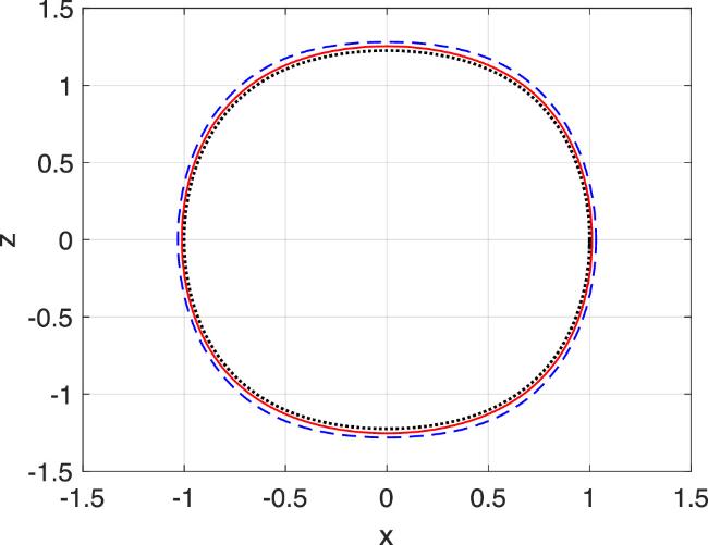
Figure 1. One typical periodic orbit of the Duffing oscillator equation ( |
Exactly the same results could be obtained with the well-known multi-timescale method [52, 53] as shown in appendix A . Nevertheless, at each order, the multi-scale method needs to introduce a ‘new’ time to cancel secular terms. Furthermore, the approximation accurate up to the mth order requires a computation to the (m + 1)th order in order to utilize the resonance condition, which can be extremely tedious when m is not small. In contrast, the concise and straightforward RG procedure is easy to proceed to higher orders, without introducing any new timescales. As the order increases, the number of terms in the expansion quickly increases; for clarity, we relegate the higher-order calculations to appendix B .
3.2. Van der Pol oscillator
The van der Pol oscillator is a typical example of a second-order nonlinear dynamical system, proposed by van der Pol in 1927 to describe the behavior of electronic circuits [58]. In most cases, a limit cycle exists which is a global attractor. In the following, not only the limit cycle but also the transient dynamics leading to the cycle are described by the RG equation.
The van der Pol model reads 19 ) describes a linear oscillator. When ϵ > 0, the last term on the right-hand side of equation (19 ) is a dissipation if x2 > 1 but a driving otherwise. Starting from anywhere away from the origin, the system will approach a state of stable periodic oscillation where the total energy dissipation and acquisition is balanced in one period. When ϵ is small, the system is weakly nonlinear, and the RG technique could be conveniently employed to determine this limit cycle. Equation (19 ) may be transformed into a 2D dynamical system if a new variable, $z=\dot{x}$, is introduced. A new set of variables (u, v) is used to diagonalize the linear part of the equation which has eigenvalues +i and −i. The specific transformation is x = −i(u − v), z = u + v, resulting in
$\begin{eqnarray}\ddot{x}+x+\varepsilon ({x}^{2}-1)\dot{x}=0.\end{eqnarray}$
If ϵ = 0, equation ( $\begin{eqnarray}\begin{array}{rcl}\dot{u} & = & {\rm{i}}u+\frac{\varepsilon }{2}(u+{u}^{3}+v-{u}^{2}v-u{v}^{2}+{v}^{3}),\\ \dot{v} & = & -{\rm{i}}v+\frac{\varepsilon }{2}(u+{u}^{3}+v-{u}^{2}v-u{v}^{2}+{v}^{3}).\end{array}\end{eqnarray}$
With the naive expansion, we obtain a solution accurate to the first order:
$\begin{eqnarray}\displaystyle \begin{array}{rcl}{\rm{u}} & = & A({t}_{0}){{\rm{e}}}^{{\rm{i}}(t-{t}_{0})}+\varepsilon \left[-\frac{{\rm{i}}A{({t}_{0})}^{3}}{4}{{\rm{e}}}^{3{\rm{i}}(t-{t}_{0})}\right.\\ & & +\,\frac{{\rm{i}}B{({t}_{0})}^{3}}{8}{{\rm{e}}}^{-3{\rm{i}}(t-{t}_{0})}\\ & & -\,\frac{{\rm{i}}(A({t}_{0})B({t}_{0})-1)B({t}_{0})}{4}{{\rm{e}}}^{-{\rm{i}}(t-{t}_{0})}\\ & & \left.-\,\frac{(A({t}_{0})B({t}_{0})-1)A({t}_{0})}{2}(t-{t}_{0}){{\rm{e}}}^{{\rm{i}}(t-{t}_{0})}\right]+\cdots \,,\\ {\rm{v}} & = & B({t}_{0}){{\rm{e}}}^{-{\rm{i}}(t-{t}_{0})}+\varepsilon \left[\frac{-{\rm{i}}A{({t}_{0})}^{3}}{8}{{\rm{e}}}^{3{\rm{i}}(t-{t}_{0})}\right.\\ & & +\,\frac{{\rm{i}}B{({t}_{0})}^{3}}{4}{{\rm{e}}}^{-3{\rm{i}}(t-{t}_{0})}\\ & & +\,\frac{{\rm{i}}(A({t}_{0})B({t}_{0})-1)A({t}_{0})}{4}{{\rm{e}}}^{{\rm{i}}(t-{t}_{0})}\\ & & \left.-\,\frac{(A({t}_{0})B({t}_{0})-1)B({t}_{0})}{2}(t-{t}_{0}){{\rm{e}}}^{-{\rm{i}}(t-{t}_{0})}\right]+\cdots \,.\end{array}\end{eqnarray}$
It is clearly seen that, apart from the exponential function, terms of the form $(t-{t}_{0}){{\rm{e}}}^{\pm {\rm{i}}(t-{t}_{0})}$ also appear due to the existence of resonance in the nonhomogeneous linear equations at various orders.Still, based on equation (6 ), to the first order of ϵ, the RG equation is 21 ). Equation (22 ) is actually a normal form equation for the limit cycle [51]. By setting t = t0 in equation (21 ), we get the nonlinear transformation from A, B to the variables u, v
$\begin{eqnarray}\displaystyle \begin{array}{rcl}\frac{{\rm{d}}A({t}_{0})}{{\rm{d}}{t}_{0}} & = & {\rm{i}}A({t}_{0})-\varepsilon \left(\frac{{A}^{2}({t}_{0})B({t}_{0})-A({t}_{0})}{2}\right),\\ \frac{{\rm{d}}B({t}_{0})}{{\rm{d}}{t}_{0}} & = & -{\rm{i}}B({t}_{0})+\varepsilon \left(\frac{A({t}_{0}){B}^{2}({t}_{0})-B({t}_{0})}{2}\right),\end{array}\end{eqnarray}$
where the nonlinear term results from the resonance in equation ( $\begin{eqnarray}\begin{array}{rcl}u & = & A+\varepsilon \left(-\frac{{\rm{i}}{A}^{3}}{4}-\frac{{\rm{i}}(A{B}^{2}-B)}{4}+\frac{{\rm{i}}{B}^{3}}{8}\right),\\ v & = & B+\varepsilon \left(\frac{{\rm{i}}{A}^{3}}{8}+\frac{{\rm{i}}({A}^{2}B-A)}{4}-\frac{{\rm{i}}{B}^{3}}{4}\right).\end{array}\end{eqnarray}$
To ensure the realness of x, z, the variables A, B should be complex conjugates.The substitution of equation (7 ) into equation (22 ) results in a simpler expression from the RG equation: 24 ) governs the change of the radius while the second gives that of the phase. In contrast to the first example, now the radius is not a constant due to the nonlinear dissipation term. To the first order, the phase changes uniformly and the radius approaches a fixed point r = 1 asymptotically except at the unstable point at the origin, which means that in the large time limit the solution of equation (22 ) approaches the limit cycle $A({t}_{0})={{\rm{e}}}^{{\rm{i}}{t}_{0}}$, $B({t}_{0})={{\rm{e}}}^{-{\rm{i}}{t}_{0}}$, if a proper initial phase is chosen.
$\begin{eqnarray}\displaystyle \begin{array}{rcl}\frac{{\rm{d}}r}{{\rm{d}}{t}_{0}} & = & \varepsilon \frac{r-{r}^{3}}{2},\\ \frac{{\rm{d}}\theta }{{\rm{d}}{t}_{0}} & = & 1.\end{array}\end{eqnarray}$
The first of equation (Similarly, a third-order expansion (the details are given in appendix C ) can be obtained,26 ) are pure imaginary which contributes to the change of the phase, while those of odd-order terms are real contributing to the change of the radius. With the substitution $A({t}_{0})=r({t}_{0}){{\rm{e}}}^{{\rm{i}}{t}_{0}}$, we have 27 ) has a stationary point at r(t0) = 0.978, indicating that the system approaches the stable limit cycle. The period can be obtained from the second of equation (27 ) and it is T = 6.5219, which compares favorably with the numerical result T = 6.5603, with an error of about 0.59%.
$\begin{eqnarray}\displaystyle \begin{array}{rcl}u & = & A({t}_{0}){{\rm{e}}}^{{\rm{i}}(t-{t}_{0})}+\varepsilon \left[-\frac{{\rm{i}}A{({t}_{0})}^{3}}{4}{{\rm{e}}}^{3{\rm{i}}(t-{t}_{0})}+\cdots \,\right]\\ & & -{\varepsilon }^{2}\left[\frac{5A{({t}_{0})}^{5}}{64}{{\rm{e}}}^{5{\rm{i}}(t-{t}_{0})}+\cdots \,\right]\\ & & +{\varepsilon }^{3}\left[\frac{7{\rm{i}}A{({t}_{0})}^{7}}{288}{{\rm{e}}}^{7{\rm{i}}(t-{t}_{0})}+\cdots \,\right]+\cdots \,,\\ v & = & B({t}_{0}){{\rm{e}}}^{-{\rm{i}}(t-{t}_{0})}+\varepsilon \left[\frac{{\rm{i}}B{({t}_{0})}^{3}}{4}{{\rm{e}}}^{-3{\rm{i}}(t-{t}_{0})}+\cdots \,\right]\\ & & -{\varepsilon }^{2}\left[\frac{5B{({t}_{0})}^{5}}{64}{{\rm{e}}}^{-5{\rm{i}}(t-{t}_{0})}+\cdots \,\right]\\ & & -{\varepsilon }^{3}\left[\frac{7{\rm{i}}B{({t}_{0})}^{7}}{288}{{\rm{e}}}^{-7{\rm{i}}(t-{t}_{0})}+\cdots \,\right]+\cdots \,,\end{array}\end{eqnarray}$
which gives $\begin{eqnarray}\displaystyle \begin{array}{rcl}\frac{{\rm{d}}A({t}_{0})}{{\rm{d}}{t}_{0}} & = & {\rm{i}}A({t}_{0})+\left(\frac{A({t}_{0})}{2}-\frac{A{({t}_{0})}^{2}B({t}_{0})}{2}\right)\varepsilon \\ & & -\,\frac{{\rm{i}}\left(\right.11B{({t}_{0})}^{2}A{({t}_{0})}^{3}-12A{({t}_{0})}^{2}B({t}_{0})+2A({t}_{0})\left)\right.{\varepsilon }^{2}}{16}\\ & & +\,\left(\frac{11B{({t}_{0})}^{2}A{({t}_{0})}^{3}}{64}-\frac{13A{({t}_{0})}^{4}B{({t}_{0})}^{3}}{128}\right.\\ & & \left.-\,\frac{3A{({t}_{0})}^{2}B({t}_{0})}{32}\right){\varepsilon }^{3},\\ \frac{{\rm{d}}B(t)}{{\rm{d}}{t}_{0}} & = & -\,{\rm{i}}B({t}_{0})+\left(\frac{B({t}_{0})}{2}-\frac{B{({t}_{0})}^{2}A({t}_{0})}{2}\right)\varepsilon \\ & & +\,\frac{{\rm{i}}\left(\right.11B{({t}_{0})}^{3}A{({t}_{0})}^{2}-12A({t}_{0})B{({t}_{0})}^{2}+2B(t)\left)\right.{\varepsilon }^{2}}{16}\\ & & +\,\left(\frac{11B{({t}_{0})}^{3}A{({t}_{0})}^{2}}{64}-\frac{13A{({t}_{0})}^{3}B{({t}_{0})}^{4}}{128}\right.\\ & & \left.-\,\frac{3B{({t}_{0})}^{2}A({t}_{0})}{32}\right){\varepsilon }^{3}.\end{array}\end{eqnarray}$
This is a normal form for the limit cycle, of a higher order. It is evident that the coefficients of even-order terms of ϵ in equation ( $\begin{eqnarray}\displaystyle \begin{array}{rcl}\dot{r}({t}_{0}) & = & r({t}_{0})\left[\frac{(-13r{({t}_{0})}^{6}+22r{({t}_{0})}^{4}-12r{({t}_{0})}^{2}){\varepsilon }^{3}}{128}\right.\\ & & \left.+\frac{(-64r{({t}_{0})}^{2}+64)\varepsilon }{128}\right],\\ \dot{\theta }({t}_{0}) & = & 1-\frac{(11r{({t}_{0})}^{4}-12r{({t}_{0})}^{2}+2)}{16}{\varepsilon }^{2}.\end{array}\end{eqnarray}$
Letting ϵ = 1, the first of equation (Similar to the previous case, we also obtain the third-order approximation of x and z and different calculations of the corresponding limit cycle at ϵ = 1 are plotted in figure 2. It can be seen that the approximation has poor performance near the turning points at the left-most and the right-most corner where the trajectory switches between a slow and fast motion while working well in other regions. By increasing the order of the calculation, the approximation rapidly converges to the benchmark numerical result. On the other hand, with decreasing value of ϵ, the approximation as expected becomes much better as shown in figure 3 at ϵ = 0.5 and ϵ = 0.1 where the results from the numerical and the RG computation just overlap.
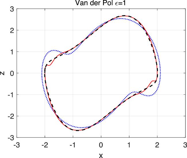
Figure 2. Limit cycle of the van der Pol oscillator at ϵ = 1 with different approaches: numerical benchmark (black dashed line), first-order RG (blue dotted line) and third-order RG (red solid line). |
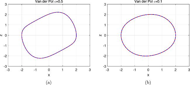
Figure 3. Limit cycles of the van der Pol equation at (a) ϵ = 0.5 and (b) ϵ = 0.1 for different computations: numerical (blue solid line) and third-order RG (red dashed line). |
3.3. Lorenz model
The Lorenz model comprises three nonlinear differential equations, serving to capture the dynamics of a simplified version of atmospheric convection. Conceived by Edward Lorenz in 1963 [59], these equations have been canonized as a paradigmatic illustration of chaotic systems. This model is an important milestone in complexity science, which takes the following form with the commonly used parameter values $\delta =28,\sigma =10,\beta =\frac{8}{3}$:
$\begin{eqnarray}\begin{array}{rcl}\dot{x} & = & \sigma (y-x),\\ \dot{y} & = & \delta x-y-xz,\\ \dot{z} & = & xy-\beta z.\end{array}\end{eqnarray}$
Note that the equation is invariant under the transformation x → −x, y → −y. Apparently, there are three fixed points: P± with ${x}_{\pm }=\pm \sqrt{\frac{8}{3}(\delta -1)},{y}_{\pm }=\pm \sqrt{\frac{8}{3}(\delta -1)},{z}_{\pm }=\delta -1$ for δ ≥ 1 and Q with x* = 0, y* = 0, z* = 0. The equilibrium Q at the origin remains stable for 1 > δ > 0 until P± are born at δ = 1 through a supercritical pitchfork bifurcation. Two unstable limit cycles are born in the homoclinic explosion at δ = 13.926 and keep shrinking with increase in δ and finally get swallowed by P± at δ = 24.74, leaving the strange set as the only attractor in the phase space. In this paper, we are interested in the limit cycle when it moves toward the equilibrium P±. Similar to the Van der Pol oscillator, at $\delta =21,\sigma =10,\beta =\frac{8}{3}$, the equations are diagonalized with a new set of variables, as follows:
$\begin{eqnarray}\begin{array}{rcl}x & = & 4\sqrt{\frac{10}{3}}-2.2414w+(0.3752+0.4457{\rm{i}})u\\ & & +(0.3752-0.4457{\rm{i}})v,\\ y & = & 4\sqrt{\frac{10}{3}}+0.7681w-\left(0.0265-0.7747{\rm{i}}\right)u\\ & & -\left(0.0265+0.7747{\rm{i}}\right)v,\\ z & = & 20+w+u+v.\end{array}\end{eqnarray}$
A perturbation expansion U = U0 + ϵU1 + ⋯ with ${U}_{0}={({x}_{+},{y}_{+},{z}_{+})}^{t}$ and ${U}_{1}={({x}_{1},{y}_{1},{z}_{1})}^{t}$ at first order gives $\begin{eqnarray}\begin{array}{rcl}{u}_{1} & = & a({t}_{0}){{\rm{e}}}^{{k}_{1}(t-{t}_{0})},\\ {v}_{1} & = & b({t}_{0}){{\rm{e}}}^{{k}_{2}(t-{t}_{0})},\\ {w}_{1} & = & c({t}_{0}){{\rm{e}}}^{{k}_{3}(t-{t}_{0})},\end{array}\end{eqnarray}$
where the free parameters a(t0), b(t0) are complex conjugates and c(t0) is real. The rates of the exponential k1 = − 0.12001 + 8.9123i, k2 = − 0.12001 − 8.9123i and k3 = − 13.4266 are the three eigenvalues of the stability matrix. All the real parts of the eigenvalues are negative, which indicates the stability of fixed point P+. The first two are conjugate to each other, signaling a spiraling motion.The sought limit cycle is related to the paired complex eigenvalues and the associated directions are described by a(t0) and b(t0). For this reason, we set c(t0) = 0. The RG computation to the third order of ϵ gives 6 ). Now, things are a little different since no eigenvalues are pure imaginary. Thus, no resonance can really occur. However, it is not hard to adapt the previous procedure to the current situation if we only check the imaginary parts of the exponents when identifying ‘resonance’ since the radial motion represented by the real parts will eventually be compensated by the nonlinear terms when approaching the limit cycle.
$\begin{eqnarray}\begin{array}{rcl}u & = & \varepsilon a({t}_{0}){{\rm{e}}}^{{k}_{1}(t-{t}_{0})}+{\varepsilon }^{2}[(0.0401+0.0419{\rm{i}})\\ & & \times a{({t}_{0})}^{2}{{\rm{e}}}^{2{k}_{1}(t-{t}_{0})}\\ & & -(0.0010-0.0052{\rm{i}})b{({t}_{0})}^{2}{{\rm{e}}}^{2{k}_{2}(t-{t}_{0})}+\cdots \,]\\ & & +{\varepsilon }^{3}[(0.0001+0.0029{\rm{i}})a{({t}_{0})}^{3}{{\rm{e}}}^{3{k}_{1}(t-{t}_{0})}\\ & & +(0.0002+0.0002{\rm{i}})b{({t}_{0})}^{3}{{\rm{e}}}^{3{k}_{2}(t-{t}_{0})}+\cdots \,]\\ & & +\cdots \,,\\ v & = & \varepsilon b({t}_{0}){{\rm{e}}}^{{k}_{2}(t-{t}_{0})}+{\varepsilon }^{2}[(-0.0010-0.0052{\rm{i}})\\ & & \times a{({t}_{0})}^{2}{{\rm{e}}}^{2{k}_{1}(t-{t}_{0})}\\ & & +(0.0401-0.0419{\rm{i}})b{({t}_{0})}^{2}{{\rm{e}}}^{2{k}_{2}(t-{t}_{0})}+\cdots \,]\\ & & +{\varepsilon }^{3}[(0.0002-0.0002{\rm{i}})a{({t}_{0})}^{3}{{\rm{e}}}^{3{k}_{1}(t-{t}_{0})}\\ & & +(0.0001-0.0029{\rm{i}})b{({t}_{0})}^{3}{{\rm{e}}}^{3{k}_{2}(t-{t}_{0})}+\cdots \,]\\ & & +\cdots \,,\\ w & = & {\varepsilon }^{2}[\left(-0.0048+0.0029{\rm{i}}\right)a{({t}_{0})}^{2}{{\rm{e}}}^{2{k}_{1}(t-{t}_{0})}+\cdots \,]\\ & & +{\varepsilon }^{3}[(-0.0004+0.00003{\rm{i}})a{({t}_{0})}^{3}{{\rm{e}}}^{3{k}_{1}(t-{t}_{0})}\\ & & +\cdots \,]+\cdots \,.\end{array}\end{eqnarray}$
During the solution of the inhomogeneous linear equation at each order, two integration constants arise. In previous examples, the eigenvalues are pure imaginary so that the solution contains not only exponential factors ${{\rm{e}}}^{-{\rm{i}}k(t-{t}_{0})}$ but also powers of t − t0 times exponentials due to resonances. In that case, all higher-order integration constants are set to zero for convenience, and the resonance terms produce nonlinear terms in dA/dt0 after they are obtained from the RG equation (With this in mind, the integration constants at higher orders could be used to nullify the ’resonance’ terms that have the same imaginary part in the exponential as that of k1 or k2, and will contribute nonlinear terms to the RG equation. With this consideration, the integration constants at even (≥2) orders of ϵ are all set to zero since there is no ’resonance’ but they have to be chosen properly at odd orders. As an example, we check the third-order terms in the expansion:
$\begin{eqnarray}\begin{array}{rcl}{u}_{3} & = & -(0.0279-0.2585{\rm{i}})a{({t}_{0})}^{2}b({t}_{0})\\ & & \times {{\rm{e}}}^{2{k}_{1}(t-{t}_{0})+{k}_{2}(t-{t}_{0})}\\ & & +(0.0008-0.0012{\rm{i}})a({t}_{0})b{({t}_{0})}^{2}\\ & & \times {{\rm{e}}}^{{k}_{1}(t-{t}_{0})+2{k}_{2}(t-{t}_{0})}\\ & & +(0.0002+0.0002{\rm{i}})b{({t}_{0})}^{3}{{\rm{e}}}^{3{k}_{2}(t-{t}_{0})}\\ & & +(0.0001+0.0029{\rm{i}})a{({t}_{0})}^{3}{{\rm{e}}}^{3{k}_{1}(t-{t}_{0})}\\ & & +{{\rm{C}}}_{31}{{\rm{e}}}^{{k}_{1}(t-{t}_{0})},\\ {v}_{3} & = & -(0.0279+0.2585{\rm{i}})a({t}_{0})b{({t}_{0})}^{2}\\ & & \times {{\rm{e}}}^{{k}_{1}(t-{t}_{0})+2{k}_{2}(t-{t}_{0})}\\ & & +(0.0008+0.0012{\rm{i}})a{({t}_{0})}^{2}b({t}_{0})\\ & & \times {{\rm{e}}}^{2{k}_{1}(t-{t}_{0})+{k}_{2}(t-{t}_{0})}\\ & & +(0.0001-0.0029{\rm{i}})b{({t}_{0})}^{3}{{\rm{e}}}^{3{k}_{2}(t-{t}_{0})}\\ & & +(0.0002-0.0002{\rm{i}})a{({t}_{0})}^{3}{{\rm{e}}}^{3{k}_{1}(t-{t}_{0})}\\ & & +{{\rm{C}}}_{32}{{\rm{e}}}^{{k}_{2}(t-{t}_{0})},\\ {w}_{3} & = & (0.0006+0.0006{\rm{i}})a({t}_{0})b{({t}_{0})}^{2}\\ & & \times {{\rm{e}}}^{{k}_{1}(t-{t}_{0})+2{k}_{2}(t-{t}_{0})}\\ & & +(0.0006-0.0006{\rm{i}})a{({t}_{0})}^{2}b({t}_{0})\\ & & \times {{\rm{e}}}^{2{k}_{1}(t-{t}_{0})+{k}_{2}(t-{t}_{0})}\\ & & -(0.0004+0.00003{\rm{i}})b{({t}_{0})}^{3}{{\rm{e}}}^{3{k}_{2}(t-{t}_{0})}\\ & & +(-0.0004+0.00003{\rm{i}})a{({t}_{0})}^{3}{{\rm{e}}}^{3{k}_{1}(t-{t}_{0})}.\end{array}\end{eqnarray}$
The first term in either of the first two equations is the abovementioned generalized resonant term since k1 + 2k2 has the same imaginary part as k2 and 2k1 + k2 as k1. The general solution of the corresponding homogeneous linear equation introduces two arbitrary constants C31, C32. According to the discussion in the previous subsection, we want these terms to disappear in the coordinate transformation but be present in the RG equation, which results in the following assignment: $\begin{eqnarray}\begin{array}{rcl}{C}_{31} & = & (0.0279-0.2585{\rm{i}})a{({t}_{0})}^{2}b({t}_{0}),\\ {C}_{32} & = & (0.0279+0.2585{\rm{i}})a({t}_{0})b{({t}_{0})}^{2}.\end{array}\end{eqnarray}$
Substituting these and equation (32 ) into equation (31 ), we get the series expansion that according to equation (6 ) leads to the following RG equation:31 ) as proposed before, which gives
$\begin{eqnarray}\begin{array}{rcl}\frac{{\rm{d}}}{{\rm{d}}{t}_{0}}a({t}_{0}) & = & (-0.1200+8.9123{\rm{i}})a({t}_{0})\\ & & +{\varepsilon }^{2}(0.0067-0.0620{\rm{i}})b({t}_{0})a{({t}_{0})}^{2},\\ \frac{{\rm{d}}}{{\rm{d}}{t}_{0}}b({t}_{0}) & = & (-0.1200-8.9123{\rm{i}})b({t}_{0})\\ & & +{\varepsilon }^{2}(0.0067+0.0620{\rm{i}})a({t}_{0})b{({t}_{0})}^{2},\end{array}\end{eqnarray}$
where b(t0) is the complex conjugate of a(t0). The nonlinear transformation from a(t0), b(t0) to u, v, w is obtained by setting t = t0 in equation ( $\begin{eqnarray}\begin{array}{rcl}u & = & \epsilon a({t}_{0})+{\epsilon }^{2}((0.0401+0.0419{\rm{i}})a{({t}_{0})}^{2}\\ & & -(0.0504-0.0400{\rm{i}})a({t}_{0})b({t}_{0})\\ & & -(0.0010-0.0052{\rm{i}})b{({t}_{0})}^{2})\\ & & +{\epsilon }^{3}((0.0001+0.0029{\rm{i}})a{({t}_{0})}^{3}\\ & & +(0.0008-0.0012{\rm{i}})a({t}_{0})b{({t}_{0})}^{2}\\ & & +(0.0002+0.0002{\rm{i}})b{({t}_{0})}^{3}),\\ v & = & \epsilon b({t}_{0})+{\epsilon }^{2}((0.0401-0.0419{\rm{i}})b{({t}_{0})}^{2}\\ & & -(0.0504+0.0400{\rm{i}})a({t}_{0})b({t}_{0})\\ & & +(-0.0010-0.0052{\rm{i}})a{({t}_{0})}^{2})\\ & & +{\epsilon }^{3}((0.0001-0.0029{\rm{i}})b{({t}_{0})}^{3}\\ & & +(0.0008+0.0012{\rm{i}})a{({t}_{0})}^{2}b({t}_{0})\\ & & +(0.0002-0.0002{\rm{i}})a{({t}_{0})}^{3}),\\ w & = & {\epsilon }^{2}(-0.0042a({t}_{0})b({t}_{0})-(0.0048\\ & & +0.0029{\rm{i}})b{({t}_{0})}^{2}+(-0.0048+0.0029i)a{({t}_{0})}^{2})\\ & & +{\epsilon }^{3}((0.0006-0.0006{\rm{i}})a{({t}_{0})}^{2}b({t}_{0})\\ & & +(0.0006+0.0006{\rm{i}})a({t}_{0})b{({t}_{0})}^{2}\\ & & -(0.0004+0.00003{\rm{i}})b{({t}_{0})}^{3}\\ & & +(-0.0004+0.00003{\rm{i}})a{({t}_{0})}^{3}).\end{array}\end{eqnarray}$
It is obvious that equation (34 ) is a normal form of the subcritical Hopf bifurcation where an unstable cycle gets created or annihilated. If polar coordinates a(t0) = reiθ and b(t0) = re−iθ are used, we have at ϵ = 1 a simple set of equation for the spiraling motion:34 ), and the phase change only depends on the radius with coefficients from the imaginary counterpart of equation (34 ), as expected from the normal form theory. Equation (36 ) could easily be solved analytically, and so we obtain an RG approximation for the limit cycle of the Lorenz equation. It is straightforward to go to higher orders without much complication with the current RG technique. For example, up to the fifth order we have
$\begin{eqnarray}\frac{{\rm{d}}r}{{\rm{d}}{t}_{0}}=(-0.1200+0.0067{r}^{2})r,\frac{{\rm{d}}\theta }{{\rm{d}}{t}_{0}}=8.9123-0.0620{r}^{2},\end{eqnarray}$
where the radial equation is self-contained with coefficients coming from the real part of the corresponding coefficients in equation ( $\begin{eqnarray}\displaystyle \begin{array}{rcl}\frac{{\rm{d}}}{{\rm{d}}{t}_{0}}a({t}_{0}) & = & (-0.1200+8.9123{\rm{i}})a({t}_{0})\\ & & +(0.0067-0.0620{\rm{i}})b({t}_{0})a{({t}_{0})}^{2}\\ & & +(0.00007-0.0008{\rm{i}})a{({t}_{0})}^{3}b{({t}_{0})}^{2},\\ \frac{{\rm{d}}}{{\rm{d}}{t}_{0}}b({t}_{0}) & = & (-0.1200-8.9123{\rm{i}})b({t}_{0})\\ & & +(0.0188+0.1843{\rm{i}})a({t}_{0})b{({t}_{0})}^{2}\\ & & +(0.00007+0.0008{\rm{i}})b{({t}_{0})}^{3}a{({t}_{0})}^{2},\end{array}\end{eqnarray}$
where the last fifth-order monomial is the new term. Note that the coefficient before this term is much smaller than those of previous terms, indicating a fast convergence of the expansion as shown in figure 4. There we clearly see that the third-order RG (black solid line) already gives quite a good result which sits close to the benchmark numerical solution (red solid line), while the fifth-order RG solution (blue dashed line) overlaps the numerical one. Quantitatively, the period of the numerical solution is T = 0.8163, in comparison with T = 0.8053 in the third-order approximation and T = 0.8076 in the fifth order. So, the error is about 1%, which also represents the accuracy of the computation. In fact, at these parameter values, the system is already far from the bifurcation point and the limit cycle grows quite large and deforms a lot from a circle. Nevertheless, the RG computation is still valid and the nonlinear terms seem to play an important role for this parameter value. For other parameter values, still higher-order approximation may be needed to match the numerical solution.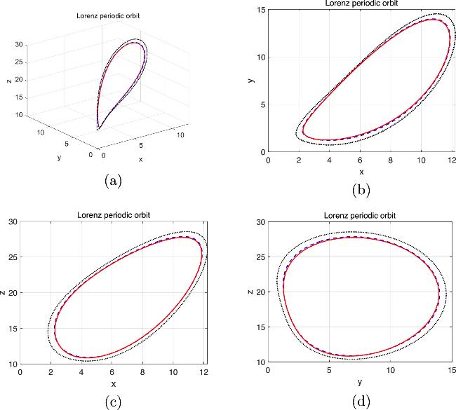
Figure 4. Limit cycle of the Lorenz system at $\delta =21,\sigma =10,\beta =\frac{8}{3}$ for different computations: benchmark numerical result (red solid line), third-order RG (black dotted line) and fifth-order RG (blue dashed line), (a) in the three-dimensional phase space, and its projections (b) in the xy-plane,(c) in the xz-plane and (d) in the yz-plane. |
4. Summary
In this paper, we have successfully employed the RG technique to identify and compute limit cycles and submanifolds in differential systems. Specifically, we have applied the RG computation to three typical physical models: the Duffing oscillator, the van der Pol oscillator, and the Lorenz model, and computed their periodic orbits. By empirically defining the resonance terms, we extended the RG method to the treatment of limit cycles in the Lorenz model with a derivation of normal forms at different orders of approximation. The calculation is especially simple and straightforward compared to the computation based on the multi-scale method.
The first example is a simple version of the well-known Duffing equation in which energy is conserved. The RG method predicts the invariance of the radius at every expansion order and each constant radius corresponds to a specific energy which also determines the period of the oscillation. Then, the method is applied to the van der Pol equation which contains both driving and dissipation. The unique limit cycle of the system is easily identified and the obtained normal form equation also captures transient trajectories approaching the limit cycle. It works well even with considerable nonlinearity. A comparison is made of the results from the RG and the multi-scale calculation, which shows that the two yield the same analytical approximation across different orders of ϵ, highlighting the effectiveness and simplicity of the RG approach.
The final example treats the Lorenz system, and we find a normal form equation for the cycles through the RG approach after the concept of ‘resonance’ is extended to complex frequencies. The approximation works well over a large range of parameter values. These examples show that the RG method can be conveniently used to efficiently compute periodic orbits in disparate contexts. With an increase of the cycle size, higher-order terms are often needed to give a good approximation, which ‘renormalize’ both the locus and the period of the orbit.
It is not hard to generalize the current procedure to the detection of periodic orbits in nonlinear systems with time delay or external driving [54]. Nevertheless, it seems hard to use the current version of the RG to treat cycles embedded in strange attractors like those in the Lorenz system in the chaotic regime [60]. There limit cycles are generated through a homoclinic explosion but not through a Hopf bifurcation and the cycles have a nontrivial shape, so it is not clear where to start the computation. The same thing happens if the linearization of a nonlinear system yields a null matrix. In these cases, smart nonlinear transformations may be needed to revive the RG technique. On the other hand, it is conceivable that invariant tori may be computed with the RG approach if more frequencies are properly recruited to the computation. In all, the great power of the RG method is yet to be uncovered for the treatment of nonlinear systems so commonly encountered in today’s science and engineering [61–64].
Appendix A.Determining periodic orbits in the Duffing oscillator using a multi-scale scheme
Here, we use the multi-time technique to compute periodic orbits in the Duffing oscillator for comparison with the RG method.
In the multi-scale approach, to obtain the nth order approximation of the period, we need to introduce n independent slow time variables [52, 53], in contrast to the straightforward computation of the RG method. For a second-order computation, we introduce multiple timescales τ = t, T = ϵt, L = ϵ2t, and the traditional perturbation expansion x = x0 + ϵx1 + ϵ2x2. After substituting these into equation (8 ), we obtain differential equations at the zeroth and the first-order of ϵ:
$\begin{eqnarray}\displaystyle \frac{{\partial }^{2}}{\partial {\tau }^{2}}{x}_{0}+{x}_{0}=0,\end{eqnarray}$
$\begin{eqnarray}\displaystyle {\partial }_{{\tau }^{2}}{x}_{1}+{x}_{1}=-{x}_{0}^{3}-2{\partial }_{\tau T}{x}_{0}.\end{eqnarray}$
The general solution of equation (A1 ) isA3 ) should be rewritten as
$\begin{eqnarray}\displaystyle {x}_{0}=A\sin (\tau )+B\cos (\tau ),\end{eqnarray}$
where A, B are integration constants with respect to τ. However, in regard to multiple independent time variables, they are actually functions of (T, L). Hence, more precisely, equation ( $\begin{eqnarray}{x}_{0}=A(T,L){\rm{\sin }}(\tau )+B(T,L){\rm{\cos }}(\tau ).\end{eqnarray}$
Substituting equation (A4 ) into equation (A2 ) results in A5 ) have the same frequency as the x1-oscillation and are thus called resonance terms. They contribute a linearly increasing amplitude to the oscillation and hence are also named secular terms, which destroy the periodicity of the solution. To maintain the cyclic behavior, we have to eliminate these terms by setting their coefficients to zero, resulting in a system of differential equations for A(T, L), B(T, L):
$\begin{eqnarray}\displaystyle \begin{array}{rcl}{\partial }_{{\tau }^{2}}{x}_{1}+{x}_{1} & = & -{x}_{0}^{3}-2{\partial }_{\tau T}{x}_{0}\\ & = & (2{\partial }_{T}B(T,L)-\frac{3}{4}A{(T,L)}^{3}\\ & & -\frac{3}{4}A(T,L)B{(T,L)}^{2}){\rm{\sin }}(\tau )\\ & & +(-2{\partial }_{T}A(T,L)-\frac{3}{4}B{(T,L)}^{3}\\ & & -\frac{3}{4}A{(T,L)}^{2}B(T,L)){\rm{\cos }}(\tau )\\ & & +{\rm{\sin }}(3\tau )\left(-\frac{3}{4}A(T,L)B{(T,L)}^{2}\right.\left.+\frac{A{(T,L)}^{3}}{4}\right)\\ & & +{\rm{\cos }}(3\tau )\left(\frac{3}{4}A{(T,L)}^{2}B(T,L)\right.\left.-\frac{B{(T,L)}^{3}}{4}\right).\end{array}\end{eqnarray}$
The two terms ${\rm{\sin }}(\tau )$ and ${\rm{\cos }}(\tau )$ on the right-hand side of equation ( $\begin{eqnarray}\displaystyle \begin{array}{rcl}{\partial }_{T}B(T,L) & = & \frac{3}{8}A{(T,L)}^{3}+\frac{3}{8}A(T,L)B{(T,L)}^{2},\\ {\partial }_{T}A(T,L) & = & -\frac{3}{8}B{(T,L)}^{3}-\frac{3}{8}A{(T,L)}^{2}B(T,L).\end{array}\end{eqnarray}$
To solve the above equations, we use the polar coordinates $A(T,L)=r(T,L)\sin (\varphi (T,L))$, $B(T,L)\,=r(T,L)\cos (\varphi (T,L))$ and find that A8 ), we are able to write a more detailed expression for x0: A2 ) gives
$\begin{eqnarray}\begin{array}{rcl}{\partial }_{T}r(T,L) & = & 0,\\ {\partial }_{T}\varphi (T,L) & = & -\frac{3}{8}r{(T,L)}^{2},\end{array}\end{eqnarray}$
which can be solved directly: $\begin{eqnarray}\begin{array}{rcl}r(T,L) & = & C(L),\\ \varphi (T,L) & = & -\frac{3}{8}C{(L)}^{2}T+D(L),\end{array}\end{eqnarray}$
where the integration constants C(L), D(L) are functions of the super-slow timescale L. With equation ( $\begin{eqnarray}\begin{array}{rcl}{x}_{0} & = & C(L)\sin \left(-\displaystyle \frac{3}{8}C{(L)}^{2}T+D(L)\right)\sin (\tau )\\ & & +C(L)\cos \left(-\displaystyle \frac{3}{8}C{(L)}^{2}T+D(L)\right)\cos (\tau )\\ & = & C(L)\cos \left(-\displaystyle \frac{3}{8}C{(L)}^{2}T+D(L)-\tau \right),\end{array}\end{eqnarray}$
a substitution of which into equation ( $\begin{eqnarray}\displaystyle \begin{array}{rcl}{\partial }_{{\tau }^{2}}{x}_{1}+{x}_{1} & = & -{x}_{0}^{3}-2{\partial }_{\tau T}{x}_{0}\\ & & -\frac{C{(L)}^{3}{\rm{\cos }}(3D(L)-\frac{9C{(L)}^{2}T}{8}-3\tau )}{4}.\end{array}\end{eqnarray}$
A particular solution of the above equation can be derived:
$\begin{eqnarray}{x}_{1}^{* }=\displaystyle \frac{C{(L)}^{3}\cos (3D(L)-\tfrac{9C{(L)}^{2}T}{8}-3\tau )}{32},\end{eqnarray}$
which contains only the high-frequency oscillation term and has eliminated the resonant terms We are now ready to solve the second-order equation: $\begin{eqnarray}\begin{array}{rcl}\frac{{\partial }^{2}}{\partial {\tau }^{2}}{x}_{2}+{x}_{2} & = & -2\frac{\partial }{\partial T}\frac{\partial }{\partial \tau }{x}_{1}(t)\\ & & -2\frac{\partial }{\partial L}\frac{\partial }{\partial \tau }{x}_{0}(t)-\frac{{\partial }^{2}}{\partial {T}^{2}}{x}_{0}(t)\\ & & -3{x}_{0}{(t)}^{2}{x}_{1}(t)\\ & = & -\frac{3C{(L)}^{5}{\rm{\cos }}\left(5D(L)-\frac{15C{(L)}^{2}T}{8}-5\tau \right)}{128}\\ & & +\,\frac{15C{(L)}^{5}{\rm{\cos }}\left(D(L)-\frac{3C{(L)}^{2}T}{8}-\tau \right)}{128}\\ & & +\,\frac{21C{(L)}^{5}{\rm{\cos }}\left(3D(L)-\frac{9C{(L)}^{2}T}{8}-3\tau \right)}{128}\\ & & -\,2C(L)\left(\frac{{\rm{d}}C(L)}{{\rm{d}}L}\right){\rm{\cos }}\left(D(L)\right.\\ & & \left.-\,\frac{3C{(L)}^{2}T}{8}-\tau \right)\\ & & -\,2\left(\frac{{\rm{d}}C(L)}{{\rm{d}}L}\right){\rm{\sin }}\left(D(L)\right.\\ & & \left.-\,\frac{3C{(L)}^{2}T}{8}-\tau \right)\\ & & +\,\frac{3C{(L)}^{2}T\left(\frac{{\rm{d}}C(L)}{{\rm{d}}L}\right){\rm{\cos }}\left(D(L)-\frac{3C{(L)}^{2}T}{8}-\tau \right)}{2}.\end{array}\end{eqnarray}$
To remove the secular terms, we set the coefficients of ${\rm{\sin }}(\tau )$ and ${\rm{\cos }}(\tau )$ to be zero:A11 ) can be found,
$\begin{eqnarray}\begin{array}{rcl}\displaystyle \frac{{\rm{d}}}{{\rm{d}}L}C(L) & = & 0,\\ \displaystyle \frac{{\rm{d}}}{{\rm{d}}L}D(L) & = & \displaystyle \frac{15C{(L)}^{4}}{256},\end{array}\end{eqnarray}$
from which we obtain C(L) = r0 and $D(L)=\frac{15{r}_{0}^{4}}{256}L$. The constancy of the amplitude is still preserved. In fact, it should be preserved for all orders because of the conservation of energy. The other variable D(L) will give a modification of the frequency. After the resonant terms are removed, a particular solution for equation ( $\begin{eqnarray}\begin{array}{rcl}{x}_{2}^{* } & = & \displaystyle \frac{{r}_{0}^{5}\cos \left(-\tfrac{15}{8}{r}_{0}^{2}\varepsilon t-5t+\tfrac{75}{256}{r}_{0}^{5}{\varepsilon }^{2}t\right)}{1024}\\ & & -\displaystyle \frac{21{r}_{0}^{5}\cos \left(-\tfrac{9}{8}{r}_{0}^{2}\varepsilon t-3t+\tfrac{45}{256}{r}_{0}^{5}\right)}{1024},\end{array}\end{eqnarray}$
which retains the oscillatory character of the solution.Therefore, a substitution of equation (A13 ) into equation (A9 ) delivers the basic angular frequency $\omega =1+\frac{3}{8}\varepsilon {r}_{0}^{2}-\frac{15}{256}{r}_{0}^{4}{\varepsilon }^{2}$, which exactly matches the second-order RG result given in the main text considering the difference of a factor 2 in the definition of r0 (check the zeroth-order term in equation (12 ) and equation (A3 )). However, the computation here seems rather cumbersome and another time variable is needed if we want to go to the next order, which requires much computation. In the RG approach, it is straightforward to perform the computation to any desired order.
Appendix B.Higher-order renormalization group analysis for the Duffing oscillator
According to the RG method, a fourth-order expansion for the Duffing oscillator can be obtained:6 ), at fourth order the RG equation is
$\begin{eqnarray*}\begin{array}{rcl}x & = & A({t}_{0}){{\rm{e}}}^{{\rm{i}}(t-{t}_{0})}+B({t}_{0}){{\rm{e}}}^{-{\rm{i}}(t-{t}_{0})}\\ & & +\,\varepsilon \left[\frac{3{\rm{i}}B({t}_{0}){A}^{2}({t}_{0})}{2}(t-{t}_{0}){{\rm{e}}}^{{\rm{i}}(t-{t}_{0})}\right.\\ & & -\,\frac{3{\rm{i}}A({t}_{0}){B}^{2}({t}_{0})}{2}(t-{t}_{0}){{\rm{e}}}^{-{\rm{i}}(t-{t}_{0})}\\ & & \left.+\,\frac{{B}^{3}({t}_{0})}{8}{{\rm{e}}}^{-3{\rm{i}}(t-{t}_{0})}+\frac{{A}^{3}({t}_{0})}{8}{{\rm{e}}}^{3{\rm{i}}(t-{t}_{0})}\right]\\ & & +\,{\varepsilon }^{2}\left[\frac{{B}^{5}({t}_{0})}{64}{{\rm{e}}}^{-5{\rm{i}}(t-{t}_{0})}+\frac{{A}^{5}({t}_{0})}{64}{{\rm{e}}}^{5{\rm{i}}(t-{t}_{0})}+\ldots \right]\\ & & +\,{\varepsilon }^{3}\left[\frac{{B}^{7}({t}_{0})}{512}{{\rm{e}}}^{-7{\rm{i}}(t-{t}_{0})}+\frac{{A}^{7}({t}_{0})}{512}{{\rm{e}}}^{7{\rm{i}}(t-{t}_{0})}+\ldots \right]\\ & & +\,{\varepsilon }^{4}\left[\frac{{B}^{9}({t}_{0})}{4096}{{\rm{e}}}^{-9{\rm{i}}(t-{t}_{0})}+\frac{{A}^{9}({t}_{0})}{4096}{{\rm{e}}}^{9{\rm{i}}(t-{t}_{0})}+\ldots \right]\\ & & +\,\ldots ,\\ z & = & {\rm{i}}A({t}_{0}){{\rm{e}}}^{{\rm{i}}(t-{t}_{0})}-{\rm{i}}B({t}_{0}){{\rm{e}}}^{-{\rm{i}}(t-{t}_{0})}\\ & & +\,\varepsilon \left[-\frac{3A({t}_{0}){B}^{2}({t}_{0})}{2}(t-{t}_{0}){{\rm{e}}}^{-{\rm{i}}(t-{t}_{0})}\right.\\ & & -\,\frac{3{\rm{i}}A({t}_{0}){B}^{2}({t}_{0})}{2}{{\rm{e}}}^{-{\rm{i}}(t-{t}_{0})}\\ & & -\,\frac{3B({t}_{0}){A}^{2}({t}_{0})}{2}(t-{t}_{0}){{\rm{e}}}^{{\rm{i}}(t-{t}_{0})}\\ & & +\,\frac{3{\rm{i}}B({t}_{0}){A}^{2}({t}_{0})}{2}{{\rm{e}}}^{{\rm{i}}(t-{t}_{0})}\\ & & \left.-\,\frac{3{\rm{i}}{B}^{3}({t}_{0})}{8}{{\rm{e}}}^{-3{\rm{i}}(t-{t}_{0})}+\frac{3{\rm{i}}{A}^{3}({t}_{0})}{8}{{\rm{e}}}^{3{\rm{i}}(t-{t}_{0})}\right]\\ & & +\,{\varepsilon }^{2}\left[-\frac{5{\rm{i}}{B}^{5}({t}_{0})}{64}{{\rm{e}}}^{-5{\rm{i}}(t-{t}_{0})}\right.\\ & & \left.+\,\frac{5{\rm{i}}{A}^{5}({t}_{0})}{64}{{\rm{e}}}^{5{\rm{i}}(t-{t}_{0})}+\ldots \right]\\ & & +\,{\varepsilon }^{3}\left[-\frac{7{\rm{i}}{B}^{7}({t}_{0})}{512}{{\rm{e}}}^{-7{\rm{i}}(t-{t}_{0})}\right.\\ & & \left.+\,\frac{7{\rm{i}}{A}^{7}({t}_{0})}{512}{{\rm{e}}}^{7{\rm{i}}(t-{t}_{0})}+\ldots \right]\\ & & +\,{\varepsilon }^{4}\left[-\frac{9{\rm{i}}{B}^{9}({t}_{0})}{4096}{{\rm{e}}}^{-9{\rm{i}}(t-{t}_{0})}\right.\\ & & \left.+\,\frac{9{\rm{i}}{A}^{9}({t}_{0})}{4096}{{\rm{e}}}^{9{\rm{i}}(t-{t}_{0})}+\ldots \right]+\ldots .\end{array}\end{eqnarray*}$
Based on equation ( $\begin{eqnarray}\displaystyle \begin{array}{rcl}\frac{{\rm{d}}A({t}_{0})}{{\rm{d}}{t}_{0}} & = & {\rm{i}}A({t}_{0})+\frac{3{\rm{i}}}{2}\varepsilon A{({t}_{0})}^{2}B({t}_{0})\\ & & -\frac{15{\rm{i}}}{16}{\varepsilon }^{2}A{({t}_{0})}^{3}B{({t}_{0})}^{2}\\ & & +\frac{123{\rm{i}}}{128}{\varepsilon }^{3}A{({t}_{0})}^{4}B{({t}_{0})}^{3}\\ & & -\frac{921{\rm{i}}}{1024}{\varepsilon }^{2}A{({t}_{0})}^{5}B{({t}_{0})}^{4},\\ \frac{{\rm{d}}B({t}_{0})}{{\rm{d}}{t}_{0}} & = & -{\rm{i}}B({t}_{0})-\frac{3{\rm{i}}}{2}\varepsilon A({t}_{0})B{({t}_{0})}^{2}\\ & & +\frac{15{\rm{i}}}{16}{\varepsilon }^{2}A{({t}_{0})}^{2}B{({t}_{0})}^{3}\\ & & -\frac{123{\rm{i}}}{128}{\varepsilon }^{3}A{({t}_{0})}^{3}B{({t}_{0})}^{4}\\ & & +\frac{921{\rm{i}}}{1024}{\varepsilon }^{2}A{({t}_{0})}^{4}B{({t}_{0})}^{5}.\end{array}\end{eqnarray}$
With the substitution $A({t}_{0})=r({t}_{0}){{\rm{e}}}^{{\rm{i}}\theta ({t}_{0})}$ and $B({t}_{0})=r({t}_{0}){{\rm{e}}}^{-{\rm{i}}\theta ({t}_{0})}$, we have
$\begin{eqnarray}\begin{array}{rcl}\dot{{\rm{r}}}({t}_{0}) & = & 0,\\ \dot{\theta }({t}_{0}) & = & 1+\displaystyle \frac{3{r}^{2}}{2}\varepsilon -\displaystyle \frac{15}{16}{{r}}^{4}{\varepsilon }^{2}+\displaystyle \frac{123}{128}{{r}}^{6}{\varepsilon }^{3}-\displaystyle \frac{921}{1024}{{r}}^{8}{\varepsilon }^{4}.\end{array}\end{eqnarray}$
To compare with the numerical computation, we take $\varepsilon =1,{r}_{0}=\frac{1}{2}$ and find $\dot{\theta }=1.3279$ from equation (B2 ), while the numeric solution gives 1.3748, resulting in an error of 3.4%.
Appendix C.Higher-order renormalization group analysis for the van der Pol oscillator
Similarly, we have used the RG method to make higher-order approximations to the van der Pol oscillator.
A fourth-order expansion can be obtained:
$\begin{eqnarray*}\begin{array}{rcl}{u} & = & A({t}_{0}){{\rm{e}}}^{{\rm{i}}(t-{t}_{0})}+\varepsilon \left[-\displaystyle \frac{{\rm{i}}A{({t}_{0})}^{3}}{4}{{\rm{e}}}^{3{\rm{i}}(t-{t}_{0})}\right.\\ & & +\,\displaystyle \frac{{\rm{i}}B{({t}_{0})}^{3}}{8}{{\rm{e}}}^{-3{\rm{i}}(t-{t}_{0})}\\ & & -\,\displaystyle \frac{{\rm{i}}(A({t}_{0})B({t}_{0})-1)B({t}_{0})}{4}{{\rm{e}}}^{-{\rm{i}}(t-{t}_{0})}\\ & & \left.-\,\displaystyle \frac{(A({t}_{0})B({t}_{0})-1)A({t}_{0})}{2}(t-{t}_{0}){{\rm{e}}}^{{\rm{i}}(t-{t}_{0})}\right]\\ & & +\,{\varepsilon }^{2}\left[-\displaystyle \frac{5}{96}B{({t}_{0})}^{5}{{\rm{e}}}^{-5{\rm{i}}(t-{t}_{0})}\right.\\ & & \left.-\,\displaystyle \frac{5}{64}A{({t}_{0})}^{5}{{\rm{e}}}^{5i(t-{t}_{0})}+\ldots \right]\\ & & +\,{\varepsilon }^{3}\left[-\displaystyle \frac{7{\rm{i}}}{384}B{({t}_{0})}^{7}{{\rm{e}}}^{-7{\rm{i}}(t-{t}_{0})}\right.\\ & & \left.+\,\displaystyle \frac{7{\rm{i}}}{288}A{({t}_{0})}^{7}{{\rm{e}}}^{7{\rm{i}}(t-{t}_{0})}+...\right]\\ & & +\,{\varepsilon }^{4}\left[\displaystyle \frac{61}{10240}B{({t}_{0})}^{9}{{\rm{e}}}^{-9{\rm{i}}(t-{t}_{0})}\right.\\ & & \left.+\,\displaystyle \frac{61}{8192}A{({t}_{0})}^{9}{{\rm{e}}}^{9{\rm{i}}(t-{t}_{0})}+...\right]+...,\\ {\rm{v}} & = & B({t}_{0}){{\rm{e}}}^{-{\rm{i}}(t-{t}_{0})}+\varepsilon \left[\displaystyle \frac{-{\rm{i}}A{({t}_{0})}^{3}}{8}{{\rm{e}}}^{3{\rm{i}}(t-{t}_{0})}\right.\\ & & +\,\displaystyle \frac{{\rm{i}}B{({t}_{0})}^{3}}{4}{{\rm{e}}}^{-3{\rm{i}}(t-{t}_{0})}\\ & & +\,\displaystyle \frac{{\rm{i}}(A({t}_{0})B({t}_{0})-1)A({t}_{0})}{4}{{\rm{e}}}^{{\rm{i}}(t-{t}_{0})}\\ & & \left.-\,\displaystyle \frac{(A({t}_{0})B({t}_{0})-1)B({t}_{0})}{2}(t-{t}_{0}){{\rm{e}}}^{-{\rm{i}}(t-{t}_{0})}\right]\\ & & +\,{\varepsilon }^{2}\left[-\displaystyle \frac{5}{96}A{({t}_{0})}^{5}{{\rm{e}}}^{5{\rm{i}}(t-{t}_{0})}-\displaystyle \frac{5}{64}B{({t}_{0})}^{5}{{\rm{e}}}^{-5{\rm{i}}(t-{t}_{0})}+\ldots \right]\\ & & +\,{\varepsilon }^{3}\left[-\displaystyle \frac{7{\rm{i}}}{288}B{({t}_{0})}^{7}{{\rm{e}}}^{-7{\rm{i}}(t-{t}_{0})}\right.\\ & & \left.+\,\displaystyle \frac{7{\rm{i}}}{384}A{({t}_{0})}^{7}{{\rm{e}}}^{7{\rm{i}}(t-{t}_{0})}+...\right]\\ & & +\,{\varepsilon }^{4}\left[\displaystyle \frac{61}{8192}B{({t}_{0})}^{9}{{\rm{e}}}^{-9{\rm{i}}(t-{t}_{0})}\right.\\ & & \left.+\,\displaystyle \frac{61}{10240}A{({t}_{0})}^{9}{{\rm{e}}}^{9{\rm{i}}(t-{t}_{0})}+...\right],\end{array}\end{eqnarray*}$
which gives $\begin{eqnarray*}\begin{array}{rcl}\displaystyle \frac{{\rm{d}}A({t}_{0})}{{\rm{d}}{t}_{0}} & = & {\rm{i}}A({t}_{0})+\left(\displaystyle \frac{A({t}_{0})}{2}-\displaystyle \frac{A{({t}_{0})}^{2}B({t}_{0})}{2}\right)\varepsilon \\ & & -\displaystyle \frac{{\rm{i}}11B{({t}_{0})}^{2}A{({t}_{0})}^{3}-12A{({t}_{0})}^{2}B({t}_{0})+2A({t}_{0})\left)\right.{\varepsilon }^{2}}{16}\\ & & +\displaystyle \frac{11B{({t}_{0})}^{2}A{({t}_{0})}^{3}}{64}-\displaystyle \frac{13A{({t}_{0})}^{4}B{({t}_{0})}^{3}}{128}\\ & & -\displaystyle \frac{3A{({t}_{0})}^{2}B({t}_{0})}{32}{\varepsilon }^{3}\\ & & -\displaystyle \frac{{\rm{i}}A({t}_{0})(24-528A({t}_{0})B(t)+3372A{({t}_{0})}^{2}B{({t}_{0})}^{2}-6114A{({t}_{0})}^{3}B{({t}_{0})}^{3}+3319A{({t}_{0})}^{4}B{({t}_{0})}^{4})}{3072}{\varepsilon }^{4},\\ \displaystyle \frac{{\rm{d}}B({t}_{0})}{{\rm{d}}{t}_{0}} & = & -{\rm{i}}B({t}_{0})+\left(\displaystyle \frac{B({t}_{0})}{2}-\displaystyle \frac{B{({t}_{0})}^{2}A({t}_{0})}{2}\right)\varepsilon \\ & & +\displaystyle \frac{{\rm{i}}\left(11B{({t}_{0})}^{3}A{({t}_{0})}^{2}-12A({t}_{0})B{({t}_{0})}^{2}+2B({t}_{0})\right){\varepsilon }^{2}}{16}\\ & & +\displaystyle \frac{11B{({t}_{0})}^{3}A{({t}_{0})}^{2}}{64}-\displaystyle \frac{13A{(t)}^{3}B{(t)}^{4}}{128}\\ & & -\displaystyle \frac{3B{({t}_{0})}^{2}A({t}_{0})}{32}{\varepsilon }^{3}\\ & & +\displaystyle \frac{{\rm{i}}B({t}_{0})(24-528A({t}_{0})B({t}_{0})+3372A{({t}_{0})}^{2}B{({t}_{0})}^{2}-6114A{({t}_{0})}^{3}B{({t}_{0})}^{3}+3319A{({t}_{0})}^{4}B{({t}_{0})}^{4})}{3072}{\varepsilon }^{4}.\end{array}\end{eqnarray*}$
With the substitution $A({t}_{0})=r({t}_{0}){{\rm{e}}}^{{\rm{i}}\theta ({t}_{0})}$ and $B({t}_{0})=r({t}_{0}){{\rm{e}}}^{-{\rm{i}}\theta ({t}_{0})}$, we have
$\begin{eqnarray}\begin{array}{rcl}\dot{r}({t}_{0}) & = & r({t}_{0})\left[\frac{(-13r{({t}_{0})}^{6}+22r{({t}_{0})}^{4}-12r{({t}_{0})}^{2}){\varepsilon }^{3}}{128}\right.\\ & & \left.+\frac{(-64r{({t}_{0})}^{2}+64)\varepsilon }{128}\right],\\ \dot{\theta }({t}_{0}) & = & 1-\frac{(11r{({t}_{0})}^{4}-12r{({t}_{0})}^{2}+2)}{16}{\varepsilon }^{2}\\ & & +\frac{(-24+528r{({t}_{0})}^{2}-3372r{({t}_{0})}^{4}+6114r{({t}_{0})}^{6}-3319r{({t}_{0})}^{8})}{3072}{\varepsilon }^{4}.\end{array}\end{eqnarray}$
Letting ϵ = 1, the first of equation (C1 ) has a stable equilibrium point at r = 0.978, indicating that the system approaches a stable limit cycle. The period, obtained from the second of equation (C1 ), is T = 6.5974, which compares favorably with the numerical result T = 6.5603, with an error of about 0.57%.