


1. Introduction
The exact solution of nonlinear evolution equations [1, 2] plays an important role in the study of soliton and integrable system theory. There have been many results for nonlinear waves of integrable equations, but they are mainly concentrated on constant backgrounds, such as the soliton usually on a zero background, while breather waves and rogue waves are usually on a plane wave background. However, it is often not constant in a practical meaning. In nonlinear wave solutions, rogue waves can always lead to a deadly disaster. Therefore, it is very important to construct rogue periodic waves for mathematical discussion. In order to characterize real complex nonlinear wave phenomena in a multi-component nonlinear system, we establish rogue waves on a periodic background in this paper, which is our main motivation. In recent years, studies on rogue periodic waves have become popular in nonlinear science. From a theoretical point of view, these waves are regarded as rogue wave solutions for the nonlinear evolution equations (NLEEs) on the periodic background. Currently, the rogue wave solution of the NLEE has been widely studied. Among them, the rogue periodic waves generated on the background of Jacobian elliptic periodic waves have attracted more and more attention. In 2018, the initial work was pioneered by Chen and Pelinovsky [3–6]. Rogue wave solutions of the nonlinear Schr$\ddot{{\rm{o}}}$dinger (NLS) equation [3, 4] and the modified Korteweg–de Vries (mKdV) equation [5] under the background of Jacobian elliptic dn and cn-function have been established by nonlinearization of the Lax pair and the Darboux transformation method [7–15]. After that, researchers have found that several well-known nonlinear evolution equations also admitted rogue periodic wave solutions such as the derivative nonlinear Schr$\ddot{{\rm{o}}}$dinger (DNLS) equation [6], the sine-Gordon equation [16], the Hirota equation [17, 21], the Ito equation [18], the FONLS equation [19], the complex mKdV equation [20], the (3+1)-d NLS equation [22], the short pulse equation and coupled integrable dispersionless equation [23], the fourth- [24], fifth- [25], and sixth-order [26] the NLS equations, the AB system [27], the (2+1)-dimensional Myrzakulov–Lakshmanan-IV equation [28] and so on. Usually, multi-component nonlinear systems are rich in hybrid wave structures. This paper mainly examines the reduced Maxwell–Bloch system [29–31]
$\begin{eqnarray}2{q}_{t}=v,\end{eqnarray}$
$\begin{eqnarray}{u}_{x}=-\mu v,\end{eqnarray}$
$\begin{eqnarray}{v}_{x}=-2q\omega +\mu u,\end{eqnarray}$
$\begin{eqnarray}{\omega }_{x}=2qv,\end{eqnarray}$
where q(x, t), u(x, t), v(x, t), ω(x, t) are complex differentiable functions, and the subscripts denote the partial derivatives with respect to the scaled space variable x and time variable t. μ is an arbitrary constant. The reduced Maxwell-Bloch system has been studied for the N-fold Darboux transformation and soliton solutions [32]. The Darboux transformation has been proposed for finding the soliton solutions [8, 33]. The generalized Darboux transformation, which can be iterated with the same spectral parameter, has been developed to construct high-order rogue wave solutions and multi-pole soliton solutions [34, 35]. Other ways for solving nonlinear systems have been developed, such as the binary Darboux transformation [36], the Hirota method [37–43], and the Pfaffian technique [44].The main structure of this paper is as follows. In section 2 , the Lax pair of equation (1 ) is described. In section 3 , we determine admissible eigenvalues. In section 4 , we get the corresponding periodic and non-periodic eigenfunctions of the Lax pair. In section 5 , we derive the one-fold and two-fold Darboux transformations of equation (1 ). In section 6 , rogue waves of the reduced Maxwell–Bloch system on the dn-periodic background and cn-periodic background are derived by Darboux transformation and nonlinearization of the Lax pair. In section 7 , some conclusions are given.
2. The Lax pair of the reduced Maxwell–Bloch system
The Lax pair of equation (1 ) can be written in the form 1 ).
$\begin{eqnarray}{{\rm{\Phi }}}_{x}=U(\lambda ,q){\rm{\Phi }},\quad U(\lambda ,q)=\left(\begin{array}{cc}\lambda & q\\ -q & -\lambda \end{array}\right),\end{eqnarray}$
$\begin{eqnarray}\begin{array}{rcl}{{\rm{\Phi }}}_{t} & = & V(\lambda ,q){\rm{\Phi }},\\ V(\lambda ,q) & = & \frac{1}{-4{\lambda }^{2}-{\mu }^{2}}\left(\begin{array}{cc}\lambda \omega & \lambda v+\frac{1}{2}\mu u\\ \lambda v-\frac{1}{2}\mu u & -\lambda \omega \end{array}\right),\end{array}\end{eqnarray}$
where ${\rm{\Phi }}={({\phi }_{1},{\phi }_{2})}^{{\rm{T}}}$ is the vector eigenfunction, and λ is the spectral parameter. The compatibility condition Ut − Vx + UV − VU = 0 can directly give rise to equation (3. Jacobian elliptic-function solutions and Hamiltonian system
Deriving (1c ) and getting 1d ) and substituting it with (1a ), (1b ), (1d ) into the above equation to obtain 6 ) by qξ at the same time
$\begin{eqnarray}{v}_{xx}=-2{q}_{x}\omega -2q{\omega }_{x}+\mu {u}_{x},\end{eqnarray}$
integrating ( $\begin{eqnarray}2{q}_{txx}=-2{q}_{x}\left(\int 4q{q}_{t}{\rm{d}}x+{C}_{1}\right)-8{q}^{2}{q}_{t}-2{\mu }^{2}{q}_{t},\end{eqnarray}$
where C1 is a constant. Let q(x, t) = q(x − ct, k) = q(ξ, k), substituting it to the above formula and simplifying it to get $\begin{eqnarray}-2c{q}_{\xi \xi \xi }=12c{q}_{\xi }{q}^{2}+(2c{\mu }^{2}-2{C}_{1}){q}_{\xi },\end{eqnarray}$
we integrate the above equation and multiply both sides of equation ( $\begin{eqnarray}-2c{q}_{\xi \xi }{q}_{\xi }=4c{q}^{3}{q}_{\xi }+(2c{\mu }^{2}-2{C}_{1})q{q}_{\xi }+{C}_{2}{q}_{\xi },\end{eqnarray}$
where C2 is a constant, integrating the above equation (7 ) again 9 ) and (10 ) satisfy the following elliptic equation.9 ), we have b0 = 2 − k2; a0 = k2 − 1. For the cn-function solution (10 ), we have b0 = 2k2 − 1; a0 = k2 − k4. By differentiating equation (11 ) with respect to x, we obtain a second-order differential equation
$\begin{eqnarray}{q}_{\xi }^{2}=-{q}^{4}-\frac{1}{2c}(2c{\mu }^{2}-2{C}_{1}){q}^{2}-\frac{{C}_{2}}{c}q-\frac{{C}_{3}}{c},\end{eqnarray}$
where C3 is a constant. Letting C1 = C2 = 0, C3 = 1, we obtain $\begin{eqnarray}q={\rm{d}}{\rm{n}}(\xi ;k),\quad c=\frac{1}{1-{k}^{2}},\quad \mu =\pm \sqrt{{k}^{2}-2},\end{eqnarray}$
$\begin{eqnarray}q=k{\rm{c}}{\rm{n}}(\xi ;k),\quad {\rm{c}}=\frac{1}{{k}^{2}({k}^{2}-1)},\quad \mu =\pm \sqrt{1-2{k}^{2}},\end{eqnarray}$
where dn and cn are the Jacobian elliptic functions and k ∈ (0, 1) is the elliptic modulus. Periodic traveling-wave solutions ( $\begin{eqnarray}{q}_{\xi }^{2}=-{q}^{4}+{b}_{0}{q}^{2}+{a}_{0},\end{eqnarray}$
where a0 and b0 are two real constants. For the dn-function solution ( $\begin{eqnarray}{q}_{\xi \xi }+2{q}^{3}-{b}_{0}q=0.\end{eqnarray}$
By (1a )–(1d ), the periodic rogue wave solutions of u(x, t), v(x, t), ω(x, t) are related to the periodic rogue wave solutions of q(x, t) as follows
$\begin{eqnarray}v=2{q}_{t}.\end{eqnarray}$
Substituting (13 ) into (1b ) and (1d ), we have
$\begin{eqnarray}{u}_{x}=-2\mu {q}_{t},\quad {\omega }_{x}=4q{q}_{t}.\end{eqnarray}$
Under the conditions for traveling-wave solutions q = q(ξ), (13 ) and (14 ) can be written as
$\begin{eqnarray}u=2c\mu q,\quad v=-2c{q}_{\xi },\quad \omega =-2c{q}^{2}.\end{eqnarray}$
Taking the derivative of equation (16 ) with respect to x and using the spatial part of the Lax pair (2 ), we have
$\begin{eqnarray}{q}_{x}=2{\lambda }_{1}({\phi }_{1}^{2}-{\phi }_{2}^{2}).\end{eqnarray}$
By taking the derivative equation (17 ) with respect to x, we get
$\begin{eqnarray}\begin{array}{l}{q}_{xx}-2{q}^{3}-(4{\lambda }_{1}^{2}+8H)q=0,\\ \quad H({\phi }_{1},{\phi }_{2})=\frac{1}{4}{({\phi }_{1}^{2}+{\phi }_{2}^{2})}^{2}+{\lambda }_{1}{\phi }_{1}{\phi }_{2},\end{array}\end{eqnarray}$
where H is a Hamiltonian function satisfying the following finite-dimensional Hamiltonian system $\begin{eqnarray}\frac{{\rm{d}}{\phi }_{1}}{{\rm{d}}x}=\frac{\partial H}{\partial {\phi }_{2}},\quad \frac{{\rm{d}}{\phi }_{2}}{{\rm{d}}x}=-\frac{\partial H}{\partial {\phi }_{1}}.\end{eqnarray}$
The following equations are obtained through rigorous collation and precise calculations
$\begin{eqnarray}{\phi }_{1}^{2}-{\phi }_{2}^{2}=\frac{1}{2{\lambda }_{1}}{q}_{x},\quad {\phi }_{1}{\phi }_{2}=\frac{1}{4{\lambda }_{1}}(4H-{q}^{2}).\end{eqnarray}$
By comparing equations (12 ) and (18 ), we find that ${b}_{0}=4{\lambda }_{1}^{2}+8H.$
The Hamiltonian system (19 ) allows the following Lax representation [45, 46]
$\begin{eqnarray}\begin{array}{rcl}U & = & \left(\begin{array}{cc}\lambda & {\phi }_{1}^{2}+{\phi }_{2}^{2}\\ -{\phi }_{1}^{2}-{\phi }_{2}^{2} & -\lambda \end{array}\right),\\ N & = & \left(\begin{array}{cc}{W}_{11}(\lambda ) & {W}_{12}(\lambda )\\ -{W}_{12}(-\lambda ) & -{W}_{11}(-\lambda )\end{array}\right),\end{array}\end{eqnarray}$
with $\begin{eqnarray*}\begin{array}{rcl}{W}_{11}(\lambda ) & = & 1-\frac{{\phi }_{1}{\phi }_{2}}{\lambda -{\lambda }_{1}}+\frac{{\phi }_{1}{\phi }_{2}}{\lambda +{\lambda }_{1}},\\ {W}_{12}(\lambda ) & = & \frac{{\phi }_{1}^{2}}{\lambda -{\lambda }_{1}}+\frac{{\phi }_{2}^{2}}{\lambda +{\lambda }_{1}},\end{array}\end{eqnarray*}$
which can be obtained from the expression above $\begin{eqnarray}{N}_{x}=[U,N].\end{eqnarray}$
Through the determinant of the matrix N, one can deduce the following differential equation 11 ) and (23 ).
$\begin{eqnarray}{q}_{x}^{2}+{q}^{4}-(4{\lambda }_{1}^{2}+8H){q}^{2}+16{H}^{2}=0,\end{eqnarray}$
which can be obtained a0 = − 16H2 from equations (For the dn-function solution (9 ), the eigenvalue λ1 takes the positive square root. The λ1 has two pairs of real values λ+ and λ− with
$\begin{eqnarray}{\lambda }_{\pm }=\frac{1}{2}(1\pm \sqrt{1-{k}^{2}}).\end{eqnarray}$
For the cn-function solution (10 ), the eigenvalue λ1 has a pair of complex-conjugate values λ+ and λ− with
$\begin{eqnarray}{\lambda }_{\pm }=\frac{1}{2}(k\pm {\rm{i}}\sqrt{1-{k}^{2}}).\end{eqnarray}$
4. Non-periodic solutions of the Lax pair
In the section, we construct the non-periodic solutions of the Lax pair (2 ) with the algebraic method. According to the work in [3], ψ1 and ψ2 have the following forms 26 ) into the Lax pair (2 ) yields
$\begin{eqnarray}{\psi }_{1}=\frac{\theta -1}{{\phi }_{2}},\quad {\psi }_{2}=\frac{\theta +1}{{\phi }_{1}},\end{eqnarray}$
where θ is a function of x and t to be determined. Inserting equation ( $\begin{eqnarray}{\theta }_{x}=q\theta \frac{{\phi }_{2}^{2}-{\phi }_{1}^{2}}{{\phi }_{1}{\phi }_{2}}+q\frac{{\phi }_{1}^{2}+{\phi }_{2}^{2}}{{\phi }_{1}{\phi }_{2}}.\end{eqnarray}$
With the use of equations (16 )–(20 ), we can rewrite equation (27 ) as 1 ) and θ0(t) is a undetermined integral function of t. Next, by placing equation (26 ) into the Lax pair (3 )
$\begin{eqnarray}{\theta }_{x}=\theta \frac{2q{q}_{x}}{{q}^{2}-4H}-\frac{4{\lambda }_{1}{q}^{2}}{{q}^{2}-4H},\end{eqnarray}$
it can be reduced to the explicit form $\begin{eqnarray}\frac{{\rm{d}}}{{\rm{d}}x}\left[\frac{\theta }{{q}^{2}-4H}\right]=-\frac{4{\lambda }_{1}{q}^{2}}{{({q}^{2}-4H)}^{2}},\end{eqnarray}$
which can be derived into the following form $\begin{eqnarray}\begin{array}{rcl}\theta (x,t) & = & -\,4{\lambda }_{1}(q{(x-ct)}^{2}-4H)\\ & & \times \left({\displaystyle \int }_{0}^{x-ct}\frac{q{(y)}^{2}}{{(q{(y)}^{2}-4H)}^{2}}{\rm{d}}y+{\theta }_{0}(t)\right),\end{array}\end{eqnarray}$
where q(y) is the solution of equation ( $\begin{eqnarray}{\theta }_{t}+c{\theta }_{x}=4{\lambda }_{1}({q}^{2}-4H)d,\end{eqnarray}$
where $\begin{eqnarray*}d=\frac{-c}{4{\lambda }_{1}^{2}+{\mu }^{2}}.\end{eqnarray*}$
By the transformation θ = − 4λ1(q2 − 4H)ρ, hence ρ satisfies 30 ), θ can take the following form
$\begin{eqnarray}{\rho }_{t}=-c{\rho }_{x}-d,\end{eqnarray}$
hence ρ(x, t) = − dt + f(x − ct), by combining with equation ( $\begin{eqnarray}\begin{array}{rcl}\theta (x,t) & = & -\,4{\lambda }_{1}(q{(x-ct)}^{2}-4H)\\ & & \times \left({\displaystyle \int }_{0}^{x-ct}\frac{q{(y)}^{2}}{{(q{(y)}^{2}-4H)}^{2}}{\rm{d}}y-dt\right).\end{array}\end{eqnarray}$
5. Darboux transformation
On the basis of the Lax pair (2 )–(3 ), in this section, we begin to construct the Darboux transformation of equation 1 . First, we derive the gauge transformation of the Lax pair (2 )–(3 ) as follows
$\begin{eqnarray}{{\rm{\Psi }}}^{{\prime} }=M{\rm{\Psi }},\end{eqnarray}$
and ${{\rm{\Psi }}}^{{\prime} }$ must be satisfied $\begin{eqnarray}{{\rm{\Psi }}}_{x}^{{\prime} }={U}^{{}^{{\prime} }}{{\rm{\Psi }}}^{{}^{{\prime} }},\quad {M}_{x}+MU={U}^{{}^{{\prime} }}M,\end{eqnarray}$
$\begin{eqnarray}{{\rm{\Psi }}}_{t}^{{\prime} }={V}^{{}^{{\prime} }}{{\rm{\Psi }}}^{{}^{{\prime} }},\quad {M}_{t}+MV={V}^{{}^{{\prime} }}M.\end{eqnarray}$
Next, let M take the following form
$\begin{eqnarray}M=M(\lambda )=\left(\begin{array}{cc}A & B\\ C & D\end{array}\right),\end{eqnarray}$
where $\begin{eqnarray*}A={\lambda }^{N}+\displaystyle \sum _{l=0}^{N-1}{A}_{l}{\lambda }^{l},\quad B=\displaystyle \sum _{l=0}^{N-1}{B}_{l}{\lambda }^{l},\end{eqnarray*}$
$\begin{eqnarray*}C=\displaystyle \sum _{l=0}^{N-1}{C}_{l}{\lambda }^{l},\quad D={\lambda }^{N}+\displaystyle \sum _{l=0}^{N-1}{D}_{l}{\lambda }^{l}.\end{eqnarray*}$
Supposing $\phi (\lambda )={({\phi }_{1}(\lambda ),{\phi }_{2}(\lambda ))}^{{\rm{T}}}$ and $\psi (\lambda )\,={({\psi }_{1}(\lambda ),{\psi }_{2}(\lambda ))}^{{\rm{T}}}$ are two basic solutions of the Lax Pair (2 )–(3 ), and defining
$\begin{eqnarray}{\alpha }_{j}=\frac{{\phi }_{2}({\lambda }_{j})+{\gamma }_{j}{\psi }_{2}({\lambda }_{j})}{{\phi }_{1}({\lambda }_{j})+{\gamma }_{j}{\psi }_{1}({\lambda }_{j})},\end{eqnarray}$
we can get the following linear algebra system $\begin{eqnarray}\displaystyle \sum _{l=0}^{N-1}({A}_{l}+{B}_{l}{\alpha }_{j}){\lambda }_{j}^{l}=-{\lambda }_{j}^{N},\end{eqnarray}$
$\begin{eqnarray}\displaystyle \sum _{l=0}^{N-1}({C}_{l}+{D}_{l}{\alpha }_{j}){\lambda }_{j}^{l}=-{\alpha }_{j}{\lambda }_{j}^{N}.\end{eqnarray}$
By applying equation (35 ) and collecting the coefficients of λ we can get the potential transformation
$\begin{eqnarray}q[N]=q-2{B}_{N-1}.\end{eqnarray}$
According to [32], for N = 1 and N = 2 in equation (41 ), the one-fold and two-fold potential transformations can be represented as
$\begin{eqnarray}q[1]=q-2\frac{{{\rm{\Delta }}}_{{B}_{0}}}{{{\rm{\Delta }}}_{0}}=q+\frac{4{\lambda }_{1}{\alpha }_{1}}{1+{\alpha }_{1}^{2}},\end{eqnarray}$
where $\begin{eqnarray*}\begin{array}{rcl}{{\rm{\Delta }}}_{{B}_{0}} & = & \left|\begin{array}{cc}1 & -{\lambda }_{1}\\ -{\alpha }_{1} & -{\lambda }_{1}{\alpha }_{1}\\ \end{array}\right|,\quad {{\rm{\Delta }}}_{0}=\left|\begin{array}{cc}1 & {\alpha }_{1}\\ -{\alpha }_{1} & 1\\ \end{array}\right|,\\ {\alpha }_{1} & = & \frac{{\phi }_{2}({\lambda }_{1})}{{\phi }_{1}({\lambda }_{1})},\quad {\gamma }_{1}=0.\end{array}\end{eqnarray*}$
$\begin{eqnarray}q[2]=q-2\frac{{{\rm{\Delta }}}_{{B}_{1}}}{{{\rm{\Delta }}}_{1}},\end{eqnarray}$
where $\begin{eqnarray*}\begin{array}{rcl}{{\rm{\Delta }}}_{{B}_{1}} & = & \left|\begin{array}{cccc}1 & {\alpha }_{1} & {\lambda }_{1} & -{\lambda }_{1}^{2}\\ 1 & {\alpha }_{2} & {\lambda }_{2} & -{\lambda }_{2}^{2}\\ -{\alpha }_{1} & 1 & -{\alpha }_{1}{\lambda }_{1} & -{\alpha }_{1}{\lambda }_{1}^{2}\\ -{\alpha }_{2} & 1 & -{\alpha }_{2}{\lambda }_{2} & -{\alpha }_{2}{\lambda }_{2}^{2}\\ \end{array}\right|,\\ {{\rm{\Delta }}}_{1} & = & \left|\begin{array}{cccc}1 & {\alpha }_{1} & {\lambda }_{1} & {\alpha }_{1}{\lambda }_{1}\\ 1 & {\alpha }_{2} & {\lambda }_{2} & {\alpha }_{2}{\lambda }_{2}\\ -{\alpha }_{1} & 1 & -{\alpha }_{1}{\lambda }_{1} & {\lambda }_{1}\\ -{\alpha }_{2} & 1 & -{\alpha }_{2}{\lambda }_{2} & {\lambda }_{2}\\ \end{array}\right|,\end{array}\end{eqnarray*}$
$\begin{eqnarray*}{\alpha }_{1}=\frac{{\phi }_{2}({\lambda }_{1})}{{\phi }_{1}({\lambda }_{1})},\quad {\alpha }_{2}=\frac{{\phi }_{2}({\lambda }_{2})}{{\phi }_{1}({\lambda }_{2})},\quad {\gamma }_{j}=0\quad (j=1,2).\end{eqnarray*}$
6. Rogue waves on a periodic background
6.1. Rogue waves on the dn-periodic background
In order to obtain rogue waves on the dn-periodic background, we choose q(x, t) = dn(x − ct; k), the real eigenvalue ${\lambda }_{1}={\lambda }_{+}=\frac{1}{2}(1+\sqrt{1-{k}^{2}})$ and $H=-\frac{1}{4}\sqrt{1-{k}^{2}}$. When N = 1, inserting equation (26 ) into the one-fold Darboux transformation (42 ), then using equation (16 ) and (20 ), we obtain the rogue dn-periodic solution
$\begin{eqnarray}{q}_{{\rm{dn}}-{\rm{rogue}}}={q}_{{\rm{dn}}}+\frac{(1-{\theta }_{{\rm{dn}}}^{2})({q}_{{\rm{dn}}}^{2}+\sqrt{1-{k}^{2}})}{{q}_{{\rm{dn}}}(1+{\theta }_{{\rm{dn}}}^{2})-2{\theta }_{{\rm{dn}}}\frac{{q}_{{\rm{dn}}}^{{}^{{\prime} }}}{1+\sqrt{1-{k}^{2}}}},\end{eqnarray}$
where $\begin{eqnarray*}\begin{array}{rcl}{\theta }_{{\rm{dn}}} & = & -4{\lambda }_{1}({q}_{{\rm{dn}}}{(x-ct)}^{2}+\sqrt{1-{k}^{2}})\\ & & \times \left({\displaystyle \int }_{0}^{x-ct}\frac{{q}_{{\rm{dn}}}{(y)}^{2}}{{({q}_{{\rm{dn}}}{(y)}^{2}+\sqrt{1-{k}^{2}})}^{2}}{\rm{d}}y+\frac{1}{2{(1-{k}^{2})}^{3/2}}t\right).\end{array}\end{eqnarray*}$
Substituting (44 ) into (15 ), we can get the rogue dn-periodic waves of the four potentials.
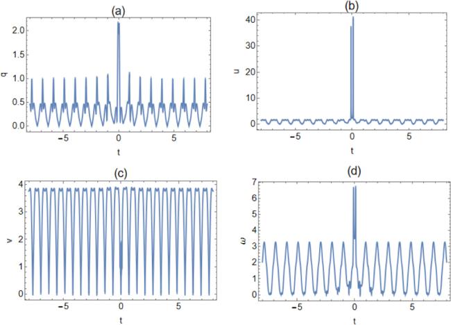
From figures 1 and 3, we can see that the rogue waves on the dn-periodic background of the reduced Maxwell–Bloch system are mainly linear rogue waves. Figures 1 and 3 illustrate the rogue dn-periodic waves with k = 0.5 and k = 0.65, respectively. From figures 2 and 4, it can be seen that, except for when the amplitude of the rogue periodic wave when v, ω = 0.5 and v, ω = 0.65 reaches the minimum value at the origin, the amplitude of the other rogue periodic waves reaches the maximum value at the origin. It can be obtained from two-dimensional figures 2 and 4, with the increase of the elliptic modulus k, the amplitude of the periodic background wave of the v is greatly reduced from 134.1 to 65.4, but the amplitude of the periodic background wave of q, u and ω increases. where the amplitude of the periodic background wave of q increases from − 0.69 to − 0.57, u increases from 0.48 to 0.5 and ω increases from 0.64 to 0.67. Therefore, the amplitude of the periodic background wave of the other potentials increases with the increase of k, except that v decreases greatly with the increase of k. That is to say, the periodic background wave amplitudes of the four potentials are regular. Moreover, from figures 2 and 4, we can see that the amplitudes of the rogue periodic waves of the four potentials are different.
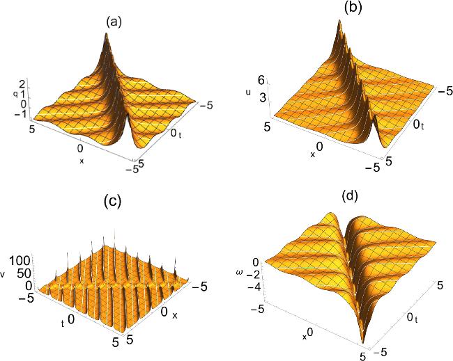
Figure 1. 3D plots of rogue waves on the dn-periodic background of the reduced Maxwell–Bloch system with k = 0.5. |
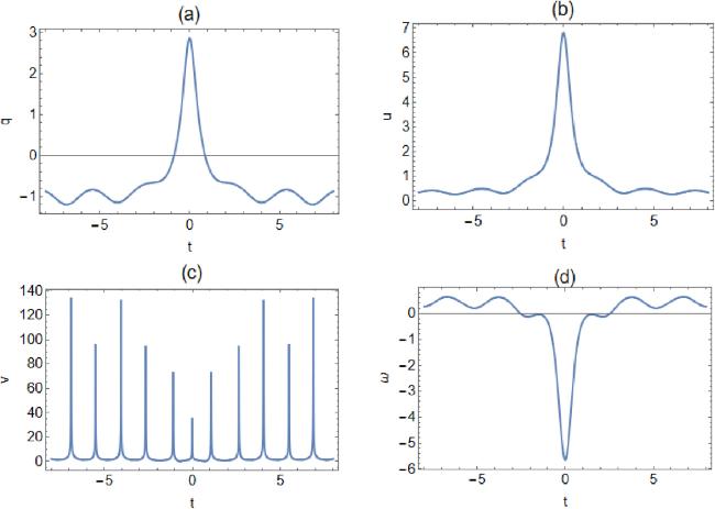
Figure 2. 2D plots of the rogue waves on the dn-periodic background with k = 0.5, x = 0. |
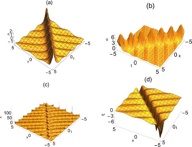
Figure 3. 3D plots of rogue waves on the dn-periodic background of the reduced Maxwell–Bloch system with k = 0.65. |
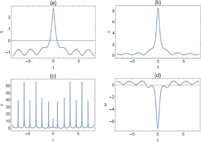
Figure 4. 2D plots of the rogue waves on the dn-periodic background with k = 0.65, x = 0. |
6.2. Rogue waves on the cn-periodic background
In order to obtain the rogue waves on the cn-periodic background, we choose q(x, t) = kcn(x − ct; k), the real eigenvalue ${\lambda }_{1}={\lambda }_{+}=\frac{1}{2}(k+{\rm{i}}\sqrt{1-{k}^{2}})$ and $H=-\frac{1}{4}{\rm{i}}k\sqrt{1-{k}^{2}}$. When N = 2, by using the two-fold Darboux transformation (43 ), equations (16 )–(20 ) and (φ1(λ1), φ2(λ1)), (φ1(λ2), φ2(λ2)) replaced by (ψ1(λ1), ψ2(λ1)), (ψ1(λ2), ψ2(λ2)), with ${\lambda }_{2}={\bar{\lambda }}_{1}$ repectively, we obtain the rogue wave on cn-periodic background solution as
$\begin{eqnarray}{q}_{{\rm{cn}}-{\rm{rogue}}}={q}_{{\rm{cn}}}+\frac{{G}_{1}}{{G}_{2}},\end{eqnarray}$
where $\begin{eqnarray*}\begin{array}{rcl}{G}_{1} & = & 4k\sqrt{1-{k}^{2}}{\rm{Im}}\left[({q}_{{\rm{cn}}}^{2}+{\rm{i}}k\sqrt{1-{k}^{2}})(1-{\theta }_{{\rm{cn}}}^{2})\right.\\ & & \left.\times [(1+{\theta }_{{\rm{cn}}}^{* }){q}_{{\rm{cn}}}-{\lambda }_{1}^{* -1}{\theta }_{{\rm{cn}}}^{* }{q}_{{\rm{cn}}}^{{}^{{\prime} }}]\right],\end{array}\end{eqnarray*}$
$\begin{eqnarray*}\begin{array}{rcl}{G}_{2} & = & (1-2{k}^{2})| (1+{\theta }_{{\rm{cn}}}^{2}){q}_{{\rm{cn}}}-{\lambda }_{1}^{-1}{\theta }_{{\rm{cn}}}{q}_{{\rm{cn}}}^{{}^{{\prime} }}{| }^{2}+| 1-{\theta }_{{\rm{cn}}}^{2}{| }^{2}\\ & & \times \left[{q}_{{\rm{cn}}}^{4}+{k}^{2}(1-{k}^{2})\right]+| (1+{\theta }_{{\rm{cn}}}^{2})\left(\frac{2}{{\lambda }_{1}}\right){q}_{{\rm{cn}}}^{{}^{{\prime} }}-2{\theta }_{{\rm{cn}}}{q}_{{\rm{cn}}}{| }^{2},\end{array}\end{eqnarray*}$
$\begin{eqnarray*}\begin{array}{rcl}{\theta }_{{\rm{cn}}} & = & -\,4{\lambda }_{1}(q{(x-ct)}^{2}+{\rm{i}}k\sqrt{1-{k}^{2}})\\ & & \times \left({\displaystyle \int }_{0}^{x-ct}\frac{{q}_{{\rm{cn}}}{(y)}^{2}}{{({q}_{{\rm{cn}}}{(y)}^{2}+{\rm{i}}k\sqrt{1-{k}^{2}})}^{2}}{\rm{d}}y-\frac{{\rm{i}}}{2{k}^{3}{(1-{k}^{2})}^{3/2}}t\right).\end{array}\end{eqnarray*}$
Substituting (45 ) into (15 ), the rogue waves on the cn-periodic background of the four potentials can be obtained.
Figures 5 and 7 illustrate the rogue cn-periodic waves for k = 0.5 and k = 0.65. From figure 6 and 8, it can be seen that except for the amplitude of the rogue periodic wave when v = 0.5 and v = 0.65 reaches the minimum value at the origin, the amplitude of the other rogue periodic waves reaches the maximum value at the origin. The corresponding two-dimensional plots are presented in figures 6 and 8. As the elliptic modulus k increases, the amplitude of the periodic background wave of q decreases from 1.01 to 0.98, u decreases from 3.52 to 1.7, v increases from 3.6 to 3.82 and ω increases from 2.43 to 3.27. With the increase of k, the amplitude of the periodic background waves of q and u decreases, and the amplitude of v and ω increases, so the amplitude of the periodic background wave of the four potentials is regular.
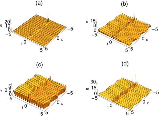
Figure 5. 3D plots of rogue waves on the cn-periodic background of the reduced Maxwell–Bloch system with k = 0.5. |
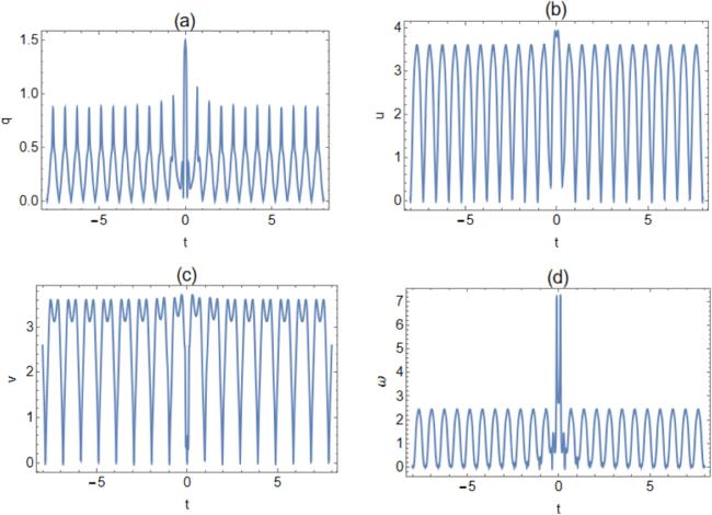
Figure 6. 2D plots of the rogue waves on the cn-periodic background with k = 0.5, x = 0. |
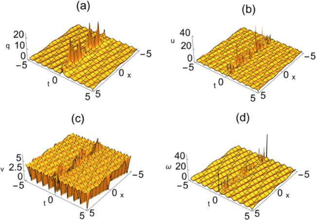
Figure 7. 3D plots of rogue waves on the cn-periodic background of the reduced Maxwell–Bloch system with k = 0.65. |
Figure 8. 2D plots of the rogue waves on the cn-periodic background with k = 0.65, x = 0. |
7. Conclusion
In this paper, we mainly study the rogue wave solution of four components of NLEEs which have Jacobian elliptic-function dn- and cn-periodic backgrounds. Compared with the existing literature, the periodic rogue wave solutions of dn and cn studied in this paper show the state of linear rogue waves such as [6, 18, 28] and so on. With the transformation of the elliptic modulus k, the amplitudes of the four potentials are also transformed. In addition, the amplitudes of the periodic background waves of all the potentials are greater than those of the rogue waves in figure 8. Compared with [5], the rogue dn-periodic and cn-periodic waves of the reduced Maxwell–Bloch system are mainly linear rogue waves, but only the rogue dn-periodic waves of [5] are linear rogue waves. These results have considerable significance when exploring other integrable equations in the future. We hope that these results on periodic wave solutions will help readers analyze some complex physical systems and provide some ideas for other researchers.
Acknowledgments
This work was supported by the National Natural Science Foundation of China (Grant No. 12361052), the Program for Innovative Research Team in Universities of Inner Mongolia Autonomous Region (Grant No. NMGIRT2414), the Fundamental Research Funds for the Inner Mongolia Normal University, China (Grant Nos. 2022JBTD007, 2022JBXC013), Graduate Students' Research and Innovation Fund of Inner Mongolia Autonomous Region (Grant No. B20231053Z), and the Key Laboratory of Infinite-Dimensional Hamiltonian System and Its Algorithm Application (Inner Mongolia Normal University), the Ministry of Education (Grant Nos. 2023KFZR01, 2023KFZR02), the First-Class Disciplines Project, Inner Mongolia Autonomous Region, China (Grant No. YLXKZX-NSD-001).
YJZ: Methodology, writing - original draft, software, visualization, data curation.
Z: Writing - review and editing, supervision, project administration, funding acquisition.
NA: Conceptualization, formal analysis.
Declaration of competing interest
The authors declare that they have no known competing financial interests or personal relationships that could have appeared to influence the work reported in this paper.