


1. Introduction
Exceptional points (EPs) which refer to the exotic spectral degeneracies of the non-Hermitian system have attracted much attention in the past two decades [1–3]. Such points have been investigated in diverse fields including optomechanics [4–6], condensed-matter physics [7], plasmonics [8], and electronics [9] both theoretically and experimentally. In general, the standard EPs are defined as the special points at which the eigenvalues and corresponding eigenvectors of the non-Hermitian Hamiltonian coalesce simultaneously [10]. The specific algebraic property of EPs brings particular physical effects, such as enhanced response to perturbations [11–15], asymmetric backscattering [16, 17], loss-induced lasing [18], etc.
Due to the progressive loss of energy, coherence, and information in the environment, the evolution of the open quantum system is non-Hermitian [19–21]. Under the weak-coupling assumption between the system and the environment, the evolution of the open system can be described by a Lindblad master equation, which can be characterized by a non-Hermitian Liouvillian superoperator. Meanwhile, the Lindblad master equation consists of a Hermitian Hamiltonian part and a non-Hermitian dissipative evolution part [22]. According to quantum trajectory theory, supposing a system whose environment is continuously and perfectly probed, the Lindblad master equation describes the average over infinite quantum trajectories [23]. Then, the dissipative evolution part can be divided into two parts, specifically, the nonunitary evolution of the system and the quantum jumps caused by the continuous measurement performed by the environment on the system [24–26]. If one post-selects the quantum trajectories where no quantum jump occurs, the evolution of the open system can be described by an effective non-Hermitian Hamiltonian [23, 27, 28].
In open quantum systems, the majority of studies focused on the EPs of the effective non-Hermitian Hamiltonian describing the evolution of the open system without quantum jumps [4, 29], called Hamiltonian EPs (HEPs). However, the inclusion of quantum jumps can have a significant effect on the system dynamics [26]. Recently, the EPs of the systems taking into account the effect of quantum jumps have been considered in different systems, which are defined via the degeneracies of the non-Hermitian Liouvillian superoperator, called Liouvillian EPs (LEPs) [30–32]. The system exhibits LEPs when two or more eigenvalues and the corresponding eigenmatrices of the Liouvillian superoperator coalesce simultaneously [26]. Currently, the LEP has shown its applications in different areas, including quantum heat engines [32–34], quantum sensors [35], superconducting qubits [36], etc.
The boundary between quantum and classical mechanics has always been a topic of foundational interest since the birth of quantum mechanics. In order to distinguish between classical and quantum behavior, Leggett and Garg introduced the concept of macrorealism [37], which was condensed into two main assumptions: macrorealism per se and noninvasive measurability. Macrorealism per se implies that the macroscopic system is always in a macroscopically distinguishable state, and noninvasive measurability implies that measurements performed do not influence the state itself or the subsequent system dynamics. Based on these assumptions, the Leggett–Garg inequality (LGI) was proposed to clarify the validity of generalizing quantum mechanics to macroscopic systems [37–39]. Then, the violation of LGI was tested experimentally in many macroscopic quantum systems, and the quantum behavior can now be confirmed experimentally [40–46]. Recently, the no-signaling-in-time (NSIT) condition has been proposed as another formulation to test macrorealism, which can be regarded as a statistical version of noninvasive measurability [47–50]. The NSIT condition is considered a better candidate for testing macrorealism than the LGI, and the former can be violated for a larger parameter regime than the latter, generally [49–51].
In the past few years, the violation of LGI in an open quantum system has been studied, and different types of environments have been considered, including Markovian [52–55] and non-Markovian [56] environments, as well as equilibrium and nonequilibrium environments [57], etc. Recently, the unique features of non-Hermitian systems have been connected with the violation of LGI. In some recent works, the violation of LGI has been investigated in non-Hermitian parity-time (${ \mathcal P }{ \mathcal T }$) symmetric systems, and shown an enhanced violation of LGI compared to the Hermitian systems [58–63]. The HEP at which the non-Hermitian system transits from ${ \mathcal P }{ \mathcal T }$-symmetric phase into ${ \mathcal P }{ \mathcal T }$-broken phase has been considered in the studies of LGI, and has shown the maximum violation of LGI in the vicinity of HEP [59–63]. However, the LEP which refers to the degeneracy of the Liouvillian superoperator that governs the complete dynamics of the open system has not been considered in the studies of LGI. Meanwhile, the different effects of the HEP and LEP on the violation of LGI are still not clear.
In this paper, we investigate the LGI and NSIT conditions in an open system, which consists of two coupled qubits, and each qubit is weakly coupled to a thermal bath at different temperatures. We also study the effect of EPs, especially LEP, on the violation of LGI and NSIT conditions, and compare the different effects between the HEP and LEP on the violation of LGI and NSIT conditions. By post-selecting the quantum trajectories where no quantum jump occurs, we find that the system can exhibit a second-order HEP, and the parameter space is divided into an overdamped regime and an underdamped regime by the HEP. We find that both LGI and NSIT conditions can be violated in both regimes and not violated at the HEP. When we take into account the effect of quantum jumps, the system can exhibit a third-order LEP, and the parameter space can also be divided into an overdamped regime and an underdamped regime by the LEP. We find that the LGI can only be violated in the underdamped regime with large coupling strength between the qubits. The NSIT conditions can be violated in both regimes, as well as at the LEP, except in the overdamped regime with small coupling strength between the qubits. Comparing the violations of the LGI and NSIT conditions with HEP and LEP, we find that the quantum jumps would reduce the generation of coherence, enhance the decoherence, and lead to narrower parameter regimes in which the LGI and NSIT conditions are violated. Furthermore, with or without quantum jumps, the NSIT conditions can be violated in a wider parameter regime than the LGI.
The rest of this paper is organized as follows. In section 2 we introduce the model considered in this paper. In section 3 we introduce the LGI and the NSIT conditions. In section 4 we study the relationship between HEP, LEP, and the violation of the LGI, and NSIT conditions, and discuss the difference between the effects of HEP and LEP on the violation of the LGI and NSIT conditions. In section 5 we present the conclusions.
2. Model
As shown in figure 1, in this paper, we consider an open system consisting of two coupled qubits with interacting strength g, and each qubit is weakly coupled to a local Markovian bosonic bath at temperature Tk (subscript k = 1, 2) with strength γk. The Hamiltonian is
$\begin{eqnarray}\hat{H}=\displaystyle \sum _{k=1,2}\varepsilon {\hat{\sigma }}_{k}^{+}{\hat{\sigma }}_{k}^{-}+g({\hat{\sigma }}_{1}^{+}{\hat{\sigma }}_{2}^{-}+{\hat{\sigma }}_{1}^{-}{\hat{\sigma }}_{2}^{+}),\end{eqnarray}$
where ϵ is the energy gap of the qubits, and ${\hat{\sigma }}_{k}^{\pm }\,=({\hat{\sigma }}_{k}^{x}\pm \,\rm{i}\,{\hat{\sigma }}_{k}^{y})/2$ are the raising and lowering operators. For convenience, we set ℏ = kB = 1. Assuming weak interqubit interaction, and within the Born approximation, the time evolution of the system density matrix is described by the following Lindblad master equation [32, 64] $\begin{eqnarray}\dot{\rho }=-\,\rm{i}\,\left[\hat{H},\rho \right]+\displaystyle \sum _{k=1,2}{\gamma }_{k}^{+}{ \mathcal D }[{\hat{\sigma }}_{k}^{+}]\rho +\displaystyle \sum _{k=1,2}{\gamma }_{k}^{-}{ \mathcal D }[{\hat{\sigma }}_{k}^{-}]\rho .\end{eqnarray}$
The dissipation of the system is described by the superoperator in the Lindblad form ${ \mathcal D }[\hat{o}]\rho =\hat{o}\rho {\hat{o}}^{\dagger }-\{{\hat{o}}^{\dagger }\hat{o},\rho \}/2$. And ${\gamma }_{k}^{+}$ and ${\gamma }_{k}^{-}$ are the incoming and outgoing rates, respectively, depending on the coupling strength between the qubit and the bath γk, as well as the statistics of the bath, ${\gamma }_{k,B}^{+}={\gamma }_{k}{n}_{B}$ and ${\gamma }_{k,B}^{-}={\gamma }_{k}(1+{n}_{B})$. And ${n}_{B}=1/({\,\rm{e}\,}^{\varepsilon /{T}_{k}}-1)$ is the Bose–Einstein distribution [65]. The model has been studied thoroughly in the past years, and it is widely used in the studies of open quantum systems [64–67].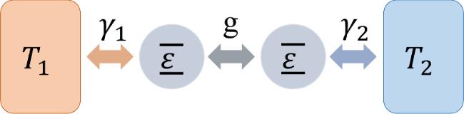
Figure 1. Sketch of the model considered in this paper, which consists of two coupled qubits with the same energy gap ϵ. Each qubit is contacted with a bosonic thermal bath with coupling strengths γ1 and γ2, respectively. The coupling strength between the qubits is g, and the temperatures of the left and right baths are T1 and T2, respectively. |
According to the theory of quantum trajectory, the dissipation terms of the Lindblad master equation can be divided into two parts: the continuous nonunitary dissipation and the quantum jumps caused by the continuous measurement performed by the environment on the system [24–26]. By rearranging the terms in the Lindblad master equation, equation (2 ) can be rewritten as 3 ) are the quantum jumps. In the classical or semiclassical regimes, the effect of the quantum jumps could be neglected directly. However, in the quantum regimes, quantum jumps have a significant effect on the dynamics of the system. If one post-selects only those trajectories where no quantum jump takes place, the master equation (3 ) becomes 5 ) can be expressed as [68]
$\begin{eqnarray}\begin{array}{rcl}\dot{\rho } & = & -\,\rm{i}\,({\hat{H}}_{\,\rm{eff}\,}\rho -\rho {\hat{H}}_{\,\rm{eff}\,}^{\dagger })\\ & & +\displaystyle \sum _{k=1,2}{\gamma }_{k}^{+}{\hat{\sigma }}_{k}^{+}\rho {\hat{\sigma }}_{k}^{-}\\ & & +\displaystyle \sum _{k=1,2}{\gamma }_{k}^{-}{\hat{\sigma }}_{k}^{-}\rho {\hat{\sigma }}_{k}^{+},\end{array}\end{eqnarray}$
where $\begin{eqnarray}{\hat{H}}_{\,\rm{eff}\,}=\hat{H}-\frac{\,\rm{i}\,}{2}\displaystyle \sum _{k=1,2}{\gamma }_{k}^{+}{\hat{\sigma }}_{k}^{-}{\hat{\sigma }}_{k}^{+}-\frac{\,\rm{i}\,}{2}\displaystyle \sum _{k=1,2}{\gamma }_{k}^{-}{\hat{\sigma }}_{k}^{+}{\hat{\sigma }}_{k}^{-}\end{eqnarray}$
is the effective non-Hermitian Hamiltonian. The last two terms in equation ( $\begin{eqnarray}\dot{\rho }=-\,\rm{i}\,({\hat{H}}_{\,\rm{eff}\,}\rho -\rho {\hat{H}}_{\,\rm{eff}\,}^{\dagger }).\end{eqnarray}$
In this way, the dynamics of the open system can be totally described by a non-Hermitian Hamiltonian ${\hat{H}}_{\,\rm{eff}\,}$, and the evolution can be regarded as a semiclassical limit of the full dynamics where the effect of quantum jumps is ignored. The general solution of the above equation equation ( $\begin{eqnarray}\rho (t)={\rm{e}\,}^{-\,\rm{i}{\hat{H}}_{\,\rm{eff}\,}t}\rho (0){\rm{e}\,}^{\,\rm{i}{\hat{H}}_{\,\rm{eff}\,}^{\dagger }t}.\end{eqnarray}$
3. LGI and NSIT condition
3.1. Leggett–Garg inequality
LGIs provide a method to investigate the existence of quantum coherence and to test the applicability of quantum mechanics [69]. Supposing a macroscopic dichotomic variable Q = ± 1 for the system, it is possible to measure its two-time correlation function
$\begin{eqnarray}{C}_{ij}=\langle Q({t}_{i})Q({t}_{j})\rangle .\end{eqnarray}$
The above correlation function is obtained from the joint probability $P({Q}_{i}^{m},{Q}_{j}^{l})$ of obtaining the results ${Q}_{i}^{m}$ and ${Q}_{j}^{l}$ (m, l = ± 1) from measurement at times ti, tj. By definition, it can be expressed as $\begin{eqnarray}{C}_{ij}=\displaystyle \sum _{m,l}{q}_{m}{q}_{l}P({Q}_{i}^{m},{Q}_{j}^{l}),\end{eqnarray}$
where qm,l = ±1 represent the outcomes of a dichotomic measurement operator Πm,l = Π±. Here, Π± characterizes a complete projection that whenever the dichotomic variable Q is measured, it is found to take one of the values ±1. Then three sets of measurements are performed to measure three different Cij with different pairs of time arguments ti and tj, where i, j = 0, 1, 2 with i < j. In the Markovian evolution, if the dynamical map of the system from ρ(s) at time s to ρ(t) at time t can be written as Λ(t − s)[ρ(s)] = ρ(t) for t > s, the correlation functions Cij can be calculated [55, 70]: $\begin{eqnarray}{C}_{ij}=\displaystyle \sum _{m,l}{q}_{m}{q}_{l}\,\rm{Tr}\,\{{{\rm{\Pi }}}_{l}{\rm{\Lambda }}({t}_{j}-{t}_{i})[{{\rm{\Pi }}}_{m}{\rm{\Lambda }}({t}_{i})\rho (0){{\rm{\Pi }}}_{m}]\}.\end{eqnarray}$
Under the assumptions of macrorealism and noninvasive measurement, the simplest LGI is defined as [69]
$\begin{eqnarray}{K}_{3}={C}_{01}+{C}_{12}-{C}_{02}\leqslant 1.\end{eqnarray}$
Since each ∣Cij∣≤1, the LGI metric K3 is algebraically bounded by ±3. The postulates of macrorealism and noninvasive measurability imply that K3≤1 for a classical system.3.2. No-signaling-in-time (NSIT) condition
The NSIT condition is another formulation to test macrorealism, which can be regarded as a statistical version of noninvasive measurability, i.e., satisfying the NSIT condition means a measurement does not change the outcome statistics of a later measurement. It provides the violation of macrorealism when one of the NSIT conditions is violated. As the NSIT condition can be violated by any nonvanishing interference term, it usually can be violated for a much wider parameter regime than the LGI [48]. The general NSIT conditions in the three-time LGI measurement scenario, which contain two-time condition NSIT and three-time condition NSIT [47–50], can be expressed as
$\begin{eqnarray}{\,\rm{NSIT}\,}_{(i)j}^{(n)m}:\quad P({Q}_{j}^{m})=\displaystyle \sum _{n}P({Q}_{i}^{n},{Q}_{j}^{m}),\end{eqnarray}$
$\begin{eqnarray}{\,\rm{NSIT}\,}_{(0)1,2}^{(n)m,l}:\quad P({Q}_{1}^{m},{Q}_{2}^{l})=\displaystyle \sum _{n}P({Q}_{0}^{n},{Q}_{1}^{m},{Q}_{2}^{l}),\end{eqnarray}$
$\begin{eqnarray}{\,\rm{NSIT}\,}_{0(1)2}^{n(m)l}:\quad P({Q}_{0}^{n},{Q}_{2}^{l})=\displaystyle \sum _{m}P({Q}_{0}^{n},{Q}_{1}^{m},{Q}_{2}^{l}),\end{eqnarray}$
where i, j = 0, 1, 2 with i < j, and n, m, l = ± 1. $P({Q}_{j}^{m})$ is the probability of obtaining outcome m by measuring at tj, and $P({Q}_{i}^{n},{Q}_{j}^{m})$ is the joint probability of obtaining outcomes n and m by measuring at ti and tj, respectively. $P({Q}_{0}^{n},{Q}_{1}^{m},{Q}_{2}^{l})$ is the joint probability of obtaining outcomes n, m and l by measuring at t0, ti and tj, respectively. The violation of the NSIT conditions can be regarded as a witness of nonclassical behavior, i.e., when one of the NSIT conditions is violated, macrorealism can be violated.
Assuming the dichotomic measurement operator Πn,m,l = Π± in the calculation of the NSIT conditions, the probabilities $P({Q}_{j}^{m})$, $P({Q}_{i}^{m},{Q}_{j}^{l})$ and $P({Q}_{0}^{n},{Q}_{1}^{m},{Q}_{2}^{l})$ can be expressed as
$\begin{eqnarray}P({Q}_{j}^{m})=\,\rm{Tr}\,[{{\rm{\Pi }}}_{m}{\rm{\Lambda }}({t}_{j})\rho (0)],\end{eqnarray}$
$\begin{eqnarray}P({Q}_{i}^{m},{Q}_{j}^{l})=\,\rm{Tr}\,\{{{\rm{\Pi }}}_{l}{\rm{\Lambda }}({t}_{j}-{t}_{i})[{{\rm{\Pi }}}_{m}{\rm{\Lambda }}({t}_{i})\rho (0){{\rm{\Pi }}}_{m}]\},\end{eqnarray}$
$\begin{eqnarray}\begin{array}{rcl}P({Q}_{0}^{n},{Q}_{1}^{m},{Q}_{2}^{l}) & = & \,\rm{Tr}\,\{{{\rm{\Pi }}}_{l}{\rm{\Lambda }}({t}_{j}-{t}_{i})[{{\rm{\Pi }}}_{m}{\rm{\Lambda }}({t}_{i}-{t}_{0})\\ & & \times [{{\rm{\Pi }}}_{n}{\rm{\Lambda }}({t}_{0})\rho (0){{\rm{\Pi }}}_{n}]{{\rm{\Pi }}}_{m}]\}.\end{array}\end{eqnarray}$
4. Result
4.1. Hamiltonian exceptional points
The evolution of the open quantum system is non-Hermitian due to the presence of dissipation, which characterizes the progressive loss of energy, coherence, and information into the environment. The presence of EP is a typical feature of non-Hermitian physics which has attracted much attention in the last two decades. The standard calculation of EPs is based on finding the degeneracy of the non-Hermitian Hamiltonian. By neglecting the effect of quantum jumps, the dynamics of the system can be described by an effective Hamiltonian. It can be seen from equation (4 ) that the effective Hamiltonian is a non-Hermitian operator, therefore, it is possible to display HEP. Supposing the eigenvalues of ${\hat{H}}_{\,\rm{eff}\,}$ are hi, and the corresponding right eigenvectors are ∣vi⟩, satisfying [26]16 ) that the HEP is not related to the temperatures of the baths, and when γ1 = γ2, the HEP $\bar{g}=0$. Figure 2 displays the imaginary parts and real parts of eigenvalues h3 and h4, as well as the scalar product of the corresponding eigenvectors ∣v3⟩ and ∣v4⟩ as functions of g. It can be seen from figure 2 that the imaginary and real parts of h3,4 are the same at $g=\bar{g}$. At the same time, the scalar product of ∣v3⟩ and ∣v4⟩ achieves 1 at $g=\bar{g}$, which indicates the presence of a second-order HEP at $g=\bar{g}$. From equation (6 ), it can be derived that the parameter space is divided into two separate regimes at the HEP $g=\bar{g}$, specifically, an overdamped regime for $g\lt \bar{g}$ without oscillation and an underdamped regime for $g\gt \bar{g}$ exhibiting oscillation. The HEP $g=\bar{g}$ corresponds to a critical point which is the boundary between the two regimes.
$\begin{eqnarray}{\hat{H}}_{\,\rm{eff}\,}| {v}_{i}\rangle ={h}_{i}| {v}_{i}\rangle ,\quad \langle {v}_{i}| {\hat{H}}_{\,\rm{eff}\,}^{\dagger }={({\hat{H}}_{\,\rm{eff}\,}| {v}_{i}\rangle )}^{\dagger }={h}_{i}^{* }\langle {v}_{i}| .\end{eqnarray}$
Then, the eigenvalues spectrum of ${\hat{H}}_{\,\rm{eff}\,}$ can be obtained as $\begin{eqnarray}\begin{array}{rcl}{h}_{1} & = & -\frac{\,\rm{i}\,}{2}({\gamma }_{1}^{+}+{\gamma }_{2}^{+});\\ {h}_{2} & = & -\frac{\,\rm{i}\,}{2}({\gamma }_{1}^{-}+{\gamma }_{2}^{-})+2\varepsilon ;\\ {h}_{3,4} & = & -\frac{\,\rm{i}\,}{4}{\rm{\Gamma }}\pm \frac{1}{2}\eta +\varepsilon ,\end{array}\end{eqnarray}$
where $\begin{eqnarray}{\rm{\Gamma }}={\gamma }_{1}^{+}+{\gamma }_{1}^{-}+{\gamma }_{2}^{+}+{\gamma }_{2}^{-},\end{eqnarray}$
$\begin{eqnarray}\eta =\sqrt{-\delta {{\rm{\Gamma }}}^{2}+4{g}^{2}},\end{eqnarray}$
with definition $\delta {\rm{\Gamma }}=[({\gamma }_{1}^{+}-{\gamma }_{1}^{-})-({\gamma }_{2}^{+}-{\gamma }_{2}^{-})]/2$. And the corresponding eigenvectors are $\begin{eqnarray}\begin{array}{l}| {{v}}_{1}\rangle ={(0\quad 0\quad 0\quad 1)}^{\,\rm{T}\,};\\ | {{v}}_{2}\rangle ={(1\quad 0\quad 0\quad 0)}^{\,\rm{T}\,};\\ | {{v}}_{3}\rangle ={\left(0\quad \frac{\,\rm{i}\,\delta {\rm{\Gamma }}+\eta }{2g}\quad 1\quad 0\right)}^{\,\rm{T}\,};\\ | {{v}}_{4}\rangle ={\left(0\quad \frac{\,\rm{i}\,\delta {\rm{\Gamma }}-\eta }{2g}\quad 1\quad 0\right)}^{\,\rm{T}\,}.\end{array}\end{eqnarray}$
It can be seen from the spectrum of ${\hat{H}}_{\,\rm{eff}\,}$ that eigenvalues h3 = h4 and the corresponding eigenvectors ∣v3⟩ = ∣v4⟩ when η = 0. Thus, the parameter which makes η = 0 is a second-order HEP of ${\hat{H}}_{\,\rm{eff}\,}$. For fixed dissipative strength γk and the temperature of the bath Tk, the HEP can be achieved by varying the coupling strength between the qubits g. When the coupling strength g equals to $\bar{g}\cong \delta {\rm{\Gamma }}/2$ which corresponds to η = 0, HEP appears. It can be derived from equation (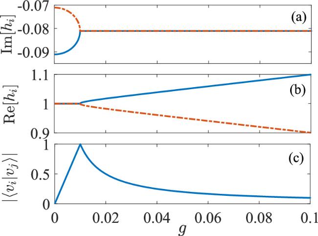
Figure 2. Spectral properties of the non-Hermitian Hamiltonian ${\hat{H}}_{\,\rm{eff}\,}$ for fixed γk. (a) The imaginary part of eigenvalues h3,4 as functions of g. (b) The real part of eigenvalues h3,4 as functions of g. (c) Scalar product between the two eigenvectors ∣v3⟩ and ∣v4⟩. The parameters are set as ϵ = 1, T1 = 3, T2 = 1, γ1 = 0.05, γ2 = 0.01, and in this case $\bar{g}=0.01$. |
In the following, we investigate the LGI in different regimes separated by the HEP $g=\bar{g}$. In this paper, we assume a pure initial state of the system ρ(0) = ∣ψ(0)⟩⟨ψ(0)∣. Let us consider a dichotomous observable $\hat{A}=2| \psi (0)\rangle \langle \psi (0)| -{\mathbb{I}}$, i.e., we ask whether the system is still in the state ∣ψ(0)⟩ (outcome + 1) or not (outcome − 1) [71]. The dichotomous observable is determined by the following projectors:
$\begin{eqnarray}\begin{array}{rcl}{{\rm{\Pi }}}_{+1} & = & | \psi (0)\rangle \langle \psi (0)| ,\\ {{\rm{\Pi }}}_{-1} & = & {\mathbb{I}}-{{\rm{\Pi }}}_{+1},\end{array}\end{eqnarray}$
where the subscripts ± 1 denote the outcomes of the projectors Π±, and ${\mathbb{I}}$ is the identity matrix.We consider a coherent initial state of the system, which is the superposition of the eigenvectors of the non-Hermitian Hamiltonian ${\hat{H}}_{\,\rm{eff}\,}$: 18 ) turns into a pair of orthogonal vectors in the space spanned by {∣01⟩, ∣10⟩}. Without loss of generality, we assume the same intermeasurement time interval t2 − t1 = t1 − t0 = τ. Then, the dynamical map of the evolution of the system from ti to tj can be expressed as 9 ) and equation (20 ). It should be noted that this evolution is not trace-preserving and needs to be normalized in the calculation.
$\begin{eqnarray}| \psi (0)\rangle =\alpha (| {v}_{3}\rangle +| {v}_{4}\rangle ),\end{eqnarray}$
where α ∈ [0, 1] is a normalization coefficient. It is worth mentioning that the initial state ∣ψ(0)⟩ considered in this paper evolves only in the space spanned by the bases {∣01⟩, ∣10⟩} during the whole evolution, thus equation ( $\begin{eqnarray}{\rm{\Lambda }}({t}_{j}-{t}_{i})[\rho ]={\rm{e}\,}^{-\,\rm{i}{\hat{H}}_{\,\rm{eff}\,}\tau }\rho \,{\rm{e}\,}^{\,\rm{i}{\hat{H}}_{\,\rm{eff}\,}^{\dagger }\tau }.\end{eqnarray}$
Then, the LGI metric K3 can be derived from equation (Figure 3(a) shows the LGI metric K3 as a function of the intermeasurement time interval τ for different coupling strength g belonging to the overdamped regime as well as g at the HEP. The blue solid, orange dash-dotted, and yellow dotted lines characterize g = 0.001, g = 0.005, and $g=\bar{g}=0.01$, respectively. For simplicity, we set t0 = 0. It can be seen from the blue solid and orange dash-dotted lines in figure 3(a) that the LGI metric K3 can be larger than 1 for $g\lt \bar{g}$, which indicates the violation of the LGI in the overdamped regime. And it can be seen from the yellow dotted line in figure 3(a) that the LGI metric K3 remains 1 for different τ, which indicates that the LGI is not violated for g at the HEP. Figure 3(b) shows the LGI metric K3 as a function of the intermeasurement time interval τ for different coupling strength g belonging to the underdamped regime. The blue solid and orange dash-dotted lines characterize g = 0.05, and g = 0.1, respectively. It can be seen from figure 3(b) that the LGI metric K3 can be larger than 1 for $g\gt \bar{g}$, which indicates the violation of the LGI in the underdamped regime. It can be found that the LGI is not violated for any intermeasurement time τ at the HEP, which indicates that the non-violation of the LGI can be regarded as a signal of the presence of HEP.
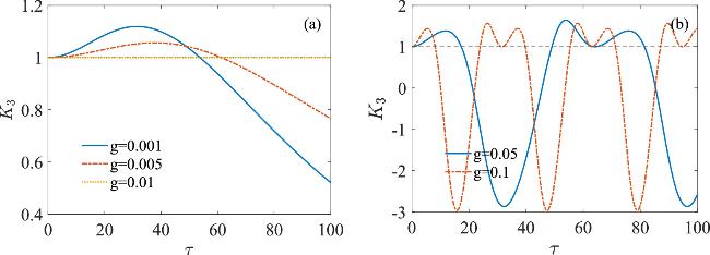
Figure 3. (a) The LGI metric K3 as a function of τ for different g in the overdamped regime ($g\lt \bar{g}$) as well as g at the HEP. The blue solid, orange dash-dotted, and yellow dotted lines characterize g = 0.001, g = 0.005, and $g=\bar{g}=0.01$, respectively. (b) The LGI metric K3 as a function of τ for different g in the underdamped regime ($g\gt \bar{g}$). The blue solid and orange dash-dotted lines characterize g = 0.05, and g = 0.1, respectively. The black dashed line characterizes K3 = 1. The other parameters are ϵ = 1, γ1 = 0.05, γ2 = 0.01, T1 = 3, T2 = 1, and t0 = 0. And in this case $\bar{g}=0.01$. |
In quantum information processing and quantum computation, coherence and entanglement are the essential ingredients, which both arise from the quantum superposition principle [72]. Additionally, quantum coherence is a more basic trait in quantum mechanics, which allows us to distinguish between classical and quantum phenomena [52]. In the following, we investigate the relation between the initial quantum coherence of the system and the violation of LGI. It can be seen from equation (17 ) that the eigenvectors of the non-Hermitian Hamiltonian ${\hat{H}}_{\,\rm{eff}\,}$∣v3⟩ and ∣v4⟩ are not orthogonal. As mentioned above, the initial state ∣ψ(0)⟩ evolves in the space spanned by the bases {∣01⟩, ∣10⟩} during the whole evolution. In order to quantify the quantum coherence of ∣ψ(0)⟩, firstly, we denote $| {v}_{3}^{\perp }\rangle $ as the orthogonal vector of ∣v3⟩ in the space spanned by the bases {∣01⟩, ∣10⟩}. Then, the initial state of the system ∣ψ(0)⟩ can be rewritten in the orthogonal bases $\{| {v}_{3}\rangle ,| {v}_{3}^{\perp }\rangle \}$ as
$\begin{eqnarray}| \psi (0)\rangle ={c}_{1}| {v}_{3}\rangle +{c}_{2}| {v}_{3}^{\perp }\rangle ,\end{eqnarray}$
where c1 = ⟨v3∣ψ(0)⟩ and ${c}_{2}=\langle {v}_{3}^{\perp }| \psi (0)\rangle $. Next, we calculate quantum coherence between ∣v3⟩ and $| {v}_{3}^{\perp }\rangle $ by using the so-called l1 norm of coherence, which is defined as the sum of the absolute values of the off-diagonal elements of the density operator ρ [73]: $\begin{eqnarray}{C}_{{l}_{1}}(\rho )=\displaystyle \sum _{i\ne j}| \langle i| \rho | j\rangle | .\end{eqnarray}$
Figure 4 displays the l1 norm of coherence ${C}_{{l}_{1}}$ between ∣v3⟩ and $| {v}_{3}^{\perp }\rangle $ as a function of the coupling strength g. It can be seen from figure 4 that the coherence decreases from 1 with the increasing of g, and reduces to 0 at $g=\bar{g}$. Then, the coherence increases to 1 gradually with the further increase of g. Compared with figure 2(c), it can be found that when the scalar product ∣⟨v3∣v4⟩∣ = 0, the eigenvectors ∣v3⟩ and ∣v4⟩ are orthogonal. Therefore, the vertical component of ∣v3⟩ of the initial state ∣ψ(0)⟩ achieves its maximum value, and the coherence between ∣v3⟩ and $| {v}_{3}^{\perp }\rangle $ is ${C}_{{l}_{1}}=1$. On the contrary, when the scalar product ∣⟨v3∣v4⟩∣ = 1, the eigenvectors ∣v3⟩ and ∣v4⟩ are coalescent. Therefore, the vertical component of ∣v3⟩ of the initial state ∣ψ(0)⟩ is 0, and the coherence between ∣v3⟩ and $| {v}_{3}^{\perp }\rangle $ is ${C}_{{l}_{1}}=0$. The HEP is a critical point corresponding to the minimum value of coherence between ∣v3⟩ and $| {v}_{3}^{\perp }\rangle $. As the coupling strength g deviates from the HEP, the vertical component of ∣v3⟩ increases gradually and leads to the increase of coherence.
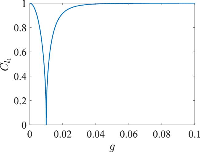
Figure 4. The l1 norm of coherence ${C}_{{l}_{1}}$ between ∣v3⟩ and $| {v}_{3}^{\perp }\rangle $ as a function of g. The parameters are set as ϵ = 1, γ1 = 0.05, γ2 = 0.01, T1 = 3, T2 = 1, and t0 = 0. And in this case $\bar{g}=0.01$. |
It has been shown that, at the HEP $g=\bar{g}$, the eigenvector ∣v3⟩ coalesces with ∣v4⟩, and the initial state of the system ∣ψ(0)⟩ turns into an eigenvector of the non-Hermitian Hamiltonian ${\hat{H}}_{\,\rm{eff}\,}$. Therefore, the system is not changed during the evolution. It can be derived from equation (9 ) that the two-time correlation functions are C01 = C12 = C02 = 1 in this situation. Thus, the LGI metric K3 remains 1, which indicates the non-violation of the LGI at the HEP $g=\bar{g}$. As the coupling strength g deviates from the HEP, the initial state of the system ∣ψ(0)⟩ is the superposition of the eigenvectors ∣v3⟩ and ∣v4⟩, which indicates a stronger quantumness of the system. Unless the initial state ρ(0) is commuted with the non-Hermitian Hamiltonian ${\hat{H}}_{\,\rm{eff}\,}$ (the density matrix and the Hamiltonian share a common set of bases), the system is always changed during the evolution which leads to the violation of the LGI. Meanwhile, the coherence of the initial state of the system ∣ψ(0)⟩ is 0 at the HEP and increases gradually as g deviates from the HEP. It can be found that the disappearance of the initial coherence of the system indicates the non-violation of the LGI, while the existence of the initial coherence indicates that the LGI can be violated. Furthermore, for a small value of τ, the degree of the violation of the LGI is enhanced as g deviates from the HEP, which indicates that the larger the initial coherence of the system, the stronger the non-classicality of the system for a short intermeasurement time interval τ. On the contrary, for a large value of τ, the decoherence during the evolution would break down the correspondence between the initial coherence and the violation of the LGI.
As shown in figure 3, the LGI metric K3 varies between greater than 1 and less than 1 as τ increases for fixed g whether in the overdamped regime or underdamped regime, which demonstrates that the LGI may change from violation to non-violation as τ evolves. It is known that the violation of LGI is closely associated with the presence of coherence in quantum systems [38]. As we know, if the density matrix of the system is commuted with the evolution operator, the system is not changed during the evolution. On the contrary, if the density matrix of the system is not commuted with the evolution operator, coherence would be generated by the dynamics. For LGI, the state of the system after measurement is determined by the projection measurement. In the following, we denote the evolution operator as $V(t)={\rm{e}\,}^{-\,\rm{i}{\hat{H}}_{\,\rm{eff}\,}t}\rho \,{\rm{e}\,}^{\,\rm{i}{\hat{H}}_{\,\rm{eff}\,}^{\dagger }t}$ and the measurement operator as M = Π+1 − Π−1, and quantify the degree of non-commutativity between the evolution operator V(t) and the measurement operator M by 23 ) is the trace distance between ρt and ${\rho }_{t}^{{\prime} }$, but it can reflect the difference that the evolution operator V(t) and the measurement operator M act on the system in different order. To some extent, equation (23 ) characterizes the degree of non-commutativity between the evolution operator V(t) and the measurement operator M.
$\begin{eqnarray}{ \mathcal D }=\frac{1}{2}\parallel {\rho }_{t}-{\rho }_{t}^{{\prime} }\parallel ,\end{eqnarray}$
where $\parallel A\parallel =\,\rm{Tr}\,\sqrt{{A}^{\dagger }A}$ denotes the trace norm. And ρt = V(t)M[ρ(0)], ${\rho }_{t}^{{\prime} }=MV(t)[\rho (0)]$ are the states that the evolution operator V(t) and the measurement operator M act on the initial state ρ(0) in different order. It is worth mentioning that M[ρ(0)] = Π+1ρ(0)Π+1 + Π−1ρ(0)Π−1 characterizes the unconditional state of the system after measurement, which is the state if one makes the measurement, but ignores the result [25]. Equation (Figure 5 demonstrates the degree of non-commutativity ${ \mathcal D }$ between the evolution operator V(t) and the measurement operator M as a function of τ for different g in different regimes. It can be seen from the blue solid and orange dash-dotted lines in figure 5(a) that ${ \mathcal D }$ is always non-zero for different τ with $g\lt \bar{g}$, which indicates that the coherence is generated by the dynamics in the overdamped regime. And it can be seen from the yellow dotted line in figure 5(a) that ${ \mathcal D }$ remains 0 for different τ with $g=\bar{g}$, which indicates that there is no coherence generated by the dynamics at the HEP. From figure 3(a), it can be seen that, in the overdamped regime, the LGI is violated for small values of τ, while not violated for large values of τ. That is because, for a long evolution time, the decoherence induced by the dissipative evolution would destroy the quantumness of the system. At the HEP, the LGI is always not violated for different τ. It can be found that when ${ \mathcal D }=0$, the LGI can not be violated, and when ${ \mathcal D }\ne 0$, the LGI might be violated. It can be seen from figure 5(b) that ${ \mathcal D }$ oscillates between 0 to 0.5 for different τ with $g\gt \bar{g}$, which indicates that the coherence is generated by the dynamics in the underdamped regime except for τ at which ${ \mathcal D }=0$. From figure 3(b), it can be found that the LGI metric K3 oscillates between − 3 to 2, which indicates that the LGI changes from violation to non-violation during the oscillation. And when ${ \mathcal D }=0$ at which there is no coherence generated by the dynamics, the LGI is always not violated. Conversely, when the LGI is violated, ${ \mathcal D }$ is always non-zero. It can be concluded that the generation of coherence is not a sufficient but a necessary condition of the violation of the LGI.
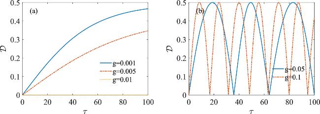
Figure 5. (a) The degree of non-commutativity between V(t) and M as a function of τ for different g in the overdamped regime ($g\lt \bar{g}$) as well as g at the HEP. The blue solid, orange dash-dotted, and yellow dotted lines characterize g = 0.001, g = 0.005, and $g=\bar{g}=0.01$, respectively. (b) The degree of non-commutativity between V(t) and M as a function of τ for different g in the underdamped regime ($g\gt \bar{g}$). The blue solid and orange dash-dotted lines characterize g = 0.05, and g = 0.1, respectively. The other parameters are the same as those in figure 3. And in this case $\bar{g}=0.01$. |
In the following, we investigate the NSIT conditions in the overdamped regime and underdamped regime separated by the HEP $g=\bar{g}$. In order to quantify the NSIT condition in equation (11a ), we denote the NSIT indicators as
$\begin{eqnarray}{\,\rm{N}\,}_{(i)j}^{(n)m}=P({Q}_{j}^{m})-\displaystyle \sum _{n}P({Q}_{i}^{n},{Q}_{j}^{m}),\end{eqnarray}$
$\begin{eqnarray}{\,\rm{N}\,}_{(0)1,2}^{(n)m,l}=P({Q}_{1}^{m},{Q}_{2}^{l})-\displaystyle \sum _{n}P({Q}_{0}^{n},{Q}_{1}^{m},{Q}_{2}^{l}),\end{eqnarray}$
$\begin{eqnarray}{\,\rm{N}\,}_{0(1)2}^{n(m)l}=P({Q}_{0}^{n},{Q}_{2}^{l})-\displaystyle \sum _{m}P({Q}_{0}^{n},{Q}_{1}^{m},{Q}_{2}^{l}).\end{eqnarray}$
${\,\rm{N}\,}_{(i)j}^{(n)m}$, ${\,\rm{N}\,}_{(0)1,2}^{(n)m,l}$, or ${\,\rm{N}\,}_{0(1)2}^{n(m)l}$ is equal to 0, which indicates the non-violation of the NSIT condition, and conversely ${\,\rm{N}\,}_{(i)j}^{(n)m}$, ${\,\rm{N}\,}_{(0)1,2}^{(n)m,l}$, or ${\,\rm{N}\,}_{0(1)2}^{n(m)l}$ does not equal to 0, which indicates the violation of the NSIT condition. In order to compare the LGI with the NSIT conditions, we choose the same dichotomic measurement operator Πn,m,l = Π± to calculate the NSIT conditions. Meanwhile, we assume the same initial state ρ(0) = ∣ψ(0)⟩⟨ψ(0)∣ and intermeasurement time interval τ.
Figure 6 shows the NSIT indicator as a function of intermeasurement time interval τ for different g in different regimes. From the numerical calculation, it is found that the NSIT conditions ${\,\rm{NSIT}\,}_{(0)1}^{(n)1}$, ${\,\rm{NSIT}\,}_{(0)2}^{(n)1}$, and ${\,\rm{NSIT}\,}_{(0)1,2}^{(n)1,1}$ are always not violated even for different parameters. Meanwhile, it should be mentioned that the non-zero NSIT indicator ${\,\rm{N}\,}_{(1)2}^{(n)1}$ and ${\,\rm{N}\,}_{0(1)2}^{1(m)1}$ have no qualitative difference. Thus, we only consider the NSIT indicator ${\,\rm{N}\,}_{0(1)2}^{1(m)1}$ here. It can be seen from the blue solid and orange dash-dotted lines in figure 6(a) that the NSIT indicator ${\,\rm{N}\,}_{0(1)2}^{1(m)1}$ can be non-zero for $g\lt \bar{g}$, which indicates the violation of NSIT condition ${\,\rm{NSIT}\,}_{0(1)2}^{1(m)1}$ in the overdamped regime. And it can be seen from the yellow dotted line in figure 6(a) that the NSIT indicator ${\,\rm{N}\,}_{0(1)2}^{1(m)1}$ remains 0 for different τ, which indicates that the NSIT condition ${\,\rm{NSIT}\,}_{0(1)2}^{1(m)1}$ is not violated for g at the HEP. It can be seen from figure 6(b) that the NSIT indicator ${\,\rm{N}\,}_{0(1)2}^{1(m)1}$ can be non-zero for $g\gt \bar{g}$, which indicates the violation of the NSIT condition ${\,\rm{NSIT}\,}_{0(1)2}^{1(m)1}$ in the underdamped regime. It should be noted that when one of the NSIT conditions is violated, the system is said to be nonclassical. Meanwhile, the NSIT condition is always non-violated at the HEP even for different τ, and this result indicates that the non-violation of the NSIT condition signals the presence of HEP. From figures 4 and 6, it can be found that when the initial coherence of the system is 0, the NSIT condition ${\,\rm{NSIT}\,}_{0(1)2}^{1(m)1}$ is not violated. When the initial coherence of the system is non-zero, the NSIT condition ${\,\rm{NSIT}\,}_{0(1)2}^{1(m)1}$ can be violated. Similar to the LGI, the degree of the violation of the NSIT condition ${\,\rm{NSIT}\,}_{0(1)2}^{1(m)1}$ is enhanced with the increasing of the initial coherence of the system as g deviates from the HEP for small τ. That indicates the non-classicality of the system is stronger with a larger initial coherence of the system for a short intermeasurement time interval τ.
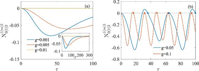
Figure 6. (a) The NSIT indicator ${\,\rm{N}\,}_{0(1)2}^{1(m)1}$ as a function of τ for different g in the overdamped regime ($g\lt \bar{g}$) as well as g at the HEP. The blue solid, orange dash-dotted, and yellow dotted lines characterize g = 0.001, g = 0.005, and $g=\bar{g}=0.01$, respectively. (b) The NSIT indicator ${\,\rm{N}\,}_{0(1)2}^{1(m)1}$ as a function of τ for different g in the underdamped regime ($g\gt \bar{g}$). The blue solid and orange dash-dotted lines characterize g = 0.05, and g = 0.1, respectively. It should be noted that the points at which the degree of non-commutativity ${ \mathcal D }=0$ are marked by the blue and orange dots. The black dashed line characterizes ${\,\rm{N}\,}_{0(1)2}^{1(m)1}=0$. The other parameters are the same as those in figure 3. And in this case $\bar{g}=0.01$. The inset of (a) shows the NSIT indicator ${\,\rm{N}\,}_{0(1)2}^{1(m)1}$ as a function of τ in a long time interval. |
It can be seen from the inset of figure 6(a) that the NSIT indicator ${\,\rm{N}\,}_{0(1)2}^{1(m)1}$ changes from less than 0 to almost 0 in a long time interval for $g\lt \bar{g}$, which indicates that the NSIT condition ${\,\rm{NSIT}\,}_{0(1)2}^{1(m)1}$ changes from violation to non-violation with the increasing of τ in the overdamped regime. From figure 5(a), it can be found that the evolution operator V(t) and the measurement operator M are not commuted in this situation, which indicates that the coherence is generated by the dynamics. However, for a long evolution time, the decoherence induced by the dissipative evolution would destroy the quantumness of the system, which induces the transition between violation and non-violation of the NSIT condition ${\,\rm{NSIT}\,}_{0(1)2}^{1(m)1}$. While at the HEP, the evolution operator V(t) and the measurement operator M are commuted for different τ, and the NSIT condition ${\,\rm{NSIT}\,}_{0(1)2}^{1(m)1}$ are always not violated. It can be seen from figure 6(b) that the NSIT indicator ${\,\rm{N}\,}_{0(1)2}^{1(m)1}$ oscillates around 0, which indicates that the NSIT condition ${\,\rm{NSIT}\,}_{0(1)2}^{1(m)1}$ varies between violation and non-violation with the increasing of τ in the underdamped regime. In figure 6(b), we mark the points at which the degree of non-commutativity ${ \mathcal D }=0$ with blue and orange dots. From figure 5(b), it can be found that when ${ \mathcal D }=0$, the NSIT condition ${\,\rm{NSIT}\,}_{0(1)2}^{1(m)1}$ is not violated, while when ${ \mathcal D }\ne 0$, the NSIT condition ${\,\rm{NSIT}\,}_{0(1)2}^{1(m)1}$ might be violated. Conversely, when the NSIT condition ${\,\rm{NSIT}\,}_{0(1)2}^{1(m)1}$ is violated, ${ \mathcal D }$ is always non-zero. It can be concluded that the generation of coherence is not a sufficient but a necessary condition of the violation of the NSIT condition. Furthermore, comparing figure 3 to figure 6, it can be found that for fixed g, when the LGI is violated, the NSIT condition is always violated. On the contrary, when the LGI is not violated, the NSIT condition can be violated. That indicates the NSIT condition can be violated in a wider time interval than the LGI. And it can be said that the NSIT condition is more sensitive as a detector of nonclassical behavior than the LGI.
4.2. Liouvillian exceptional points
The quantum jumps have been ignored according to the theory of quantum trajectory in section 4.1 . However, quantum jumps play an important role in the dynamics of open quantum systems. In this subsection, we study the LGI and NSIT conditions without ignoring quantum jumps and investigate the relation between the violation of the LGI and NSIT conditions and LEP.
In general, the Lindblad master equation can be expressed in the form $\dot{\rho }={ \mathcal L }\rho $, where ${ \mathcal L }$ is the Liouvillian superoperator. In the Liouvillian representation, the density matrix is represented by a vector in the Hilbert-Schmidt space and ${ \mathcal L }$ is a non-Hermitian matrix. A D-dimensional density matrix is represented by a D2-dimensional vector 2 ) as a matrix differential equation for vectorized state ∣ρ⟩⟩ of the density operator ρ, 26 ) is given by
$\begin{eqnarray}| \rho \rangle \rangle ={({\rho }_{1}{\rho }_{2}...{\rho }_{{D}^{2}})}^{\,\rm{T}\,},\end{eqnarray}$
where T denotes the transpose operation. Then we can recast the above master equation equation ( $\begin{eqnarray}\dot{\rho }={ \mathcal L }\rho \leftrightarrow | \dot{\rho }\rangle \rangle ={ \mathcal L }| \rho \rangle \rangle .\end{eqnarray}$
Then ${ \mathcal L }$ can be written as a (D2 × D2)-dimensional matrix. Explicitly, the matrix form of ${ \mathcal L }$ of equation ( $\begin{eqnarray}\begin{array}{rcl}{ \mathcal L } & = & -\,\rm{i}\,(H\displaystyle \otimes {\mathbb{I}}-{\mathbb{I}}\displaystyle \otimes {H}^{\,\rm{T}\,})\\ & & +\displaystyle \sum _{k=1,2}{\gamma }_{k}^{+}[{\hat{\sigma }}_{k}^{+}\displaystyle \otimes {({\hat{\sigma }}_{k}^{-})}^{\,\rm{T}\,}-\frac{1}{2}({\hat{\sigma }}_{k}^{-}\\ & & \times \,{\hat{\sigma }}_{k}^{+}\displaystyle \otimes {\mathbb{I}}+{\mathbb{I}}\displaystyle \otimes {({\hat{\sigma }}_{k}^{-}{\hat{\sigma }}_{k}^{+})}^{\,\rm{T}\,})]\\ & & +\displaystyle \sum _{k=1,2}{\gamma }_{k}^{-}[{\hat{\sigma }}_{k}^{-}\displaystyle \otimes {({\hat{\sigma }}_{k}^{+})}^{\,\rm{T}\,}\\ & & -\frac{1}{2}({\hat{\sigma }}_{k}^{+}{\hat{\sigma }}_{k}^{-}\displaystyle \otimes {\mathbb{I}}+{\mathbb{I}}\displaystyle \otimes {({\hat{\sigma }}_{k}^{+}{\hat{\sigma }}_{k}^{-})}^{\,\rm{T}\,})].\end{array}\end{eqnarray}$
Since the Liouvillian superoperator is non-Hermitian, its eigenvalue spectrum has distinct right and left eigenmatrices, which are defined by ${ \mathcal L }{\rho }_{i}={\lambda }_{i}{\rho }_{i}$ and ${{ \mathcal L }}^{\dagger }{\sigma }_{i}={\lambda }_{i}^{* }{\sigma }_{i}$, respectively. The right and left eigenmatrices form a biorthogonal basis with respect to the Hilbert-Schmidt inner product, which can be normalized by Tr[σiρj] = δij. From such a definition, the steady state of the system ρss corresponds to the eigenmatrix with eigenvalue λi = 0. Similar to HEP, Liouvillian exceptional points (LEPs) are defined as the special points at which two or more eigenvalues and corresponding eigenmatrices of the Liouvillian superoperator coalesce simultaneously [26].
It can be derived from equation (2 ) that the steady state of the system only has six non-zero elements (the populations of the four computational states and the two coherences ∣10⟩⟨01∣ and ∣01⟩⟨10∣). The initial state of the system ρ(0) considered in this subsection is the same as that in section 4.1 . It can be found that the initial state ρ(0) belongs to the steady-state subspace, therefore the Liouvillian superoperator ${ \mathcal L }$ can be reduced to 6 × 6 Liouvillian $\tilde{{ \mathcal L }}$. The exact form of the Liouvillian superoperator is provided in appendix Appendix A .
Then, the general solution of the master equation $\rho (t)={\,\rm{e}\,}^{{ \mathcal L }t}\rho (0)$ can be expressed as a weighted sum of the right eigenmatrices ρi with exponentially decaying factors:
$\begin{eqnarray}\rho (t)={\rho }_{ss}+\displaystyle \sum _{i=2}^{6}{c}_{i}{\,\rm{e}\,}^{{\lambda }_{i}t}{\rho }_{i},\end{eqnarray}$
where λi and ρi are the eigenvalue and right eigenmatrix of $\tilde{{ \mathcal L }}$. and ci = Tr[σiρ(0)] is a coefficient connected to the initial state of the system.As mentioned above, if the initial states belong to the steady-state subspace, the Liouvillian superoperator ${ \mathcal L }$ can be reduced to 6 × 6 Liouvillian $\tilde{{ \mathcal L }}$ (shown in Appendix A ). The eigenvalues of $\tilde{{ \mathcal L }}$ is shown as follows Appendix B . It can be seen from the eigenspectrum of $\tilde{{ \mathcal L }}$ that eigenvalues λ3,4 = λ5,6 at ${\eta }^{{\prime} }=0$, meanwhile, the corresponding eigenmatrices ρ4 = ρ5 = ρ6, which indicates the existence of a third-order LEP. For fixed dissipative strength γk and temperature of the reservoir Tk, the LEP can be reached by varying the coupling strength between the qubits g. When the coupling strength g equals $\tilde{g}\cong {\rm{\Delta }}{\rm{\Gamma }}/2$ which corresponds to ${\eta }^{{\prime} }=0$, LEP appears. Figure 7 shows the imaginary parts and real parts of the coalesced eigenvalues λ4, λ5 and λ6, as well as the scalar product of any two of the corresponding eigenmatrices ρ4, ρ5 and ρ6 as functions of g. Because the eigenvectors of the non-Hermitian operator are not always orthogonal, the scalar product of the eigenmatrices should be normalized in the calculation. The normalized scalar product of the eigenmatrices reaching 1 indicates the coalescence of the eigenmatrices. It can be seen from figure 7 that the imaginary and real parts of λ4,5,6 coalesce at $g=\tilde{g}\approx 0.07$. At the same time, the scalar product of any two of ρ4, ρ5 and ρ6 reaches 1 at $g=\tilde{g}$, which indicates the presence of a third-order LEP at $g=\tilde{g}$.
$\begin{eqnarray}{\lambda }_{1}=0,\quad {\lambda }_{2}=-{\rm{\Gamma }},\quad {\lambda }_{3,4}=-\frac{{\rm{\Gamma }}}{2},\quad {\lambda }_{5,6}=-\frac{{\rm{\Gamma }}}{2}\mp {\eta }^{{\prime} },\end{eqnarray}$
where $\begin{eqnarray}{\rm{\Gamma }}={{\rm{\Gamma }}}_{1}+{{\rm{\Gamma }}}_{2},\end{eqnarray}$
$\begin{eqnarray}{\eta }^{{\prime} }=\sqrt{{\rm{\Delta }}{{\rm{\Gamma }}}^{2}-4{g}^{2}},\end{eqnarray}$
with definition ${{\rm{\Gamma }}}_{k}={\gamma }_{k}^{+}+{\gamma }_{k}^{-}$, and ΔΓ = (Γ1 − Γ2)/2. The corresponding eigenmatrices can be determined analytically, and the explicit expression of ρi is given in 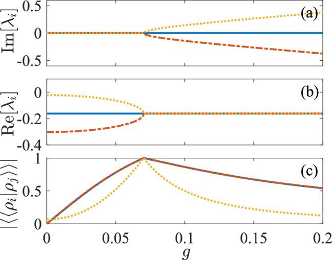
Figure 7. Spectral properties of the Liouvillian $\tilde{{ \mathcal L }}$ for fixed γk. (a) Imaginary part of eigenvalues λ4,5,6 as functions of g. (b) Real part of eigenvalues λ4,5,6 as functions of g. (c) Scalar product of any two of the corresponding eigenmatrices ρ4, ρ5 and ρ6 as functions of g. The parameters are set as ϵ = 1, T1 = 3, T2 = 1, γ1 = 0.05, γ2 = 0.01. And in this case $\tilde{g}\approx 0.07$. |
In the Liouvillian representation, the eigenvalues of the Liouvillian superoperator characterize the modes governing the dissipative dynamics. Specifically, the real part and the imaginary part of the eigenvalues λi are responsible for the decay rates and the oscillations of any expectation value towards the steady state, respectively. It can be seen from equation (29 ) that if ${\eta }^{{\prime} }$ is real, the eigenvalues of $\tilde{{ \mathcal L }}$ are all real. If ${\eta }^{{\prime} }$ is imaginary, λ5,6 becomes complex, which leads to the oscillation of the dynamics. Therefore, similar to section 4.1 , the parameter space can also be divided into two separate regimes at the LEP $g=\tilde{g}$, specifically, an overdamped regime for $g\lt \tilde{g}$ without oscillation and an underdamped regime for $g\gt \tilde{g}$ exhibiting oscillation. The LEP $g=\tilde{g}$ corresponds to a critical point which is the boundary between the two previous regimes.
In the following, we investigate the LGI in different regimes separated by the LEP $g=\tilde{g}$. In this subsection, we assume the same pure initial state of the system ρ(0) = ∣ψ(0)⟩⟨ψ(0)∣ and dichotomous observable $\hat{A}=2| \psi (0)\rangle \langle \psi (0)| -{\mathbb{I}}$ as considered in section 4.1 . It should be noted that ρ(0) = ∣ψ(0)⟩⟨ψ(0)∣ belongs to the steady-state subspace, which means that the dynamics of the system are totally determined by the Liouvillian superoperator $\tilde{{ \mathcal L }}$. Due to the effect of quantum jumps, the system would be out of the space belonging to the initial state of the system spanned by {∣0101⟩⟩, ∣0110⟩⟩, ∣1010⟩⟩, ∣1001⟩⟩} during the evolution. Without loss of generality, K3 is calculated for fixed intermeasurement time interval t2 − t1 = t1 − t0 = τ. Then, the dynamical map of the evolution of the system from ti to tj can be expressed as 9 ) and equation (32 ).
$\begin{eqnarray}{\rm{\Lambda }}({t}_{j}-{t}_{i})[\rho ]={\,\rm{e}\,}^{\tilde{{ \mathcal L }}\tau }\rho .\end{eqnarray}$
And the LGI metric K3 can be derived from equation (Figure 8 shows the LGI metric K3 as a function of the intermeasurement time interval τ for three different coupling strengths g. The blue solid, orange dash-dotted, yellow dotted, and purple dashed lines characterize g = 0.01 belonging to the overdamped regime, $g=\tilde{g}\approx 0.07$ at the LEP, and g = 0.1, g = 0.2 belonging to the underdamped regime, respectively. As in section 4.1 , we set t0 = 0. It can be seen from the blue solid and orange dash-dotted lines in figure 8 that the LGI metric K3 is always smaller than 1 for both g = 0.01 and g = 0.07, which indicates that the LGI is not violated for g belonging to the overdamped regime, as well as for g at the LEP. In the underdamped regime, it can be seen from the yellow dotted line in figure 8 corresponding to g = 0.1 that the LGI metric K3 is less than 1, which indicates the non-violation of the LGI. However, with the further increase of g, the maximum value of the LGI metric K3 increases gradually and can be larger than 1. It can be seen from the purple dashed line in figure 8 corresponding to g = 0.2 in the underdamped regime that the LGI metric K3 is larger than 1 for small τ, which indicates the violation of the LGI. While for larger τ, the LGI is not violated.
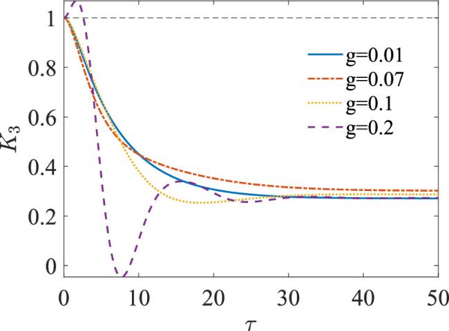
Figure 8. The LGI metric K3 as a function of τ for different coupling strength g. The blue solid, orange dash-dotted, yellow dotted, and purple dashed lines characterize g = 0.01, g = 0.07, g = 0.1, and g = 0.2, respectively. The black dashed line characterizes K3 = 1. The other parameters are set as ϵ = 1, γ1 = 0.05, γ2 = 0.01, T1 = 3, T2 = 1, and t0 = 0. And in this case $\tilde{g}\approx 0.07$. |
Similar to equation (23 ), we quantify the degree of non-commutativity between the evolution operator $W(t)={\,\rm{e}\,}^{\tilde{{ \mathcal L }}t}\rho $ and the measurement operator M without ignoring quantum jumps by
$\begin{eqnarray}{{ \mathcal D }}^{{\prime} }=\frac{1}{2}\parallel {\rho }_{t}-{\rho }_{t}^{{\prime} }\parallel ,\end{eqnarray}$
where ρt = W(t)M[ρ(0)] and ${\rho }_{t}^{{\prime} }=MW(t)[\rho (0)]$ are the states that the evolution operator W(t) and the measurement operator M act on the initial state ρ(0) in different order. It can be seen from figure 9 that ${{ \mathcal D }}^{{\prime} }$ enhances with the increasing of g, which indicates that more coherence can be generated by the dynamics with a stronger coupling strength between the qubits. That is why the LGI is not violated for small g, while can be violated for large g. Meanwhile, it can be seen from figure 9 that, for fixed g, ${{ \mathcal D }}^{{\prime} }$ decays with oscillation with the increasing of τ, which indicates that less coherence can be generated by the dynamics for larger τ. At the same time, for a large value of τ, the decoherence during the evolution would destroy the quantumness of the system, and the system changes from a pure state to a mixed state which is more classical. Therefore, the LGI changes from violation to non-violation with the increasing of τ.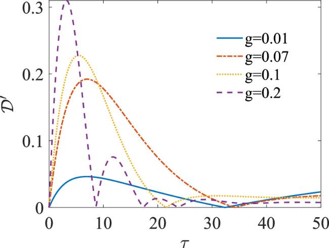
Figure 9. The degree of non-commutativity between W(t) and M as a function of τ for different g. The blue solid, orange dash-dotted, yellow dotted and purple dashed lines characterize g = 0.01, g = 0.07, g = 0.1, and g = 0.2, respectively. The other parameters are the same as those in figure 8. And in this case $\tilde{g}\approx 0.07$. |
Comparing figure 3 to figure 8, it can be found that the quantum jumps have a significant effect on the quantum-to-classical transition. When the quantum jumps are neglected by post-selecting the quantum trajectories where no quantum jump takes place, the LGI are not violated at the HEP, while violated in both overdamped and underdamped regimes. When the effect of the quantum jumps is considered, the LGI is not violated at the LEP, and not violated in the overdamped regime. In the underdamped regime, the LGI can not be violated for small g, while can be violated for large g. When the effect of quantum jumps is considered, the evolution operator W(t) is not commuted with the measurement operator M, and the coherence can be generated by the dynamics. However, the quantum jumps lead to the enhancement of decoherence, which would destroy the quantumness of the system. Thus, the LGI can be violated when the quantum jumps are ignored, but not violated when the quantum jumps are taken into account.
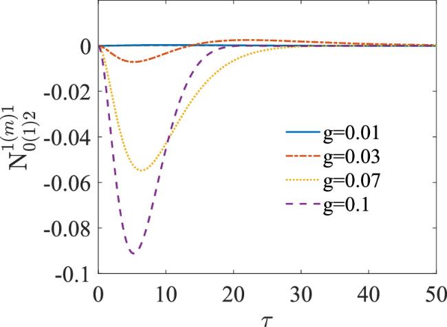
Figure 10 shows the NSIT indicator ${\,\rm{N}\,}_{0(1)2}^{1(m)1}$ as a function of intermeasurement time interval τ for different coupling strengths g. The blue solid, orange dash-dotted, yellow dotted, and purple dashed lines characterize g = 0.01 and g = 0.03 belonging to the overdamped regime, $g=\tilde{g}\approx 0.07$ at the LEP, and g = 0.1 belonging to the underdamped regime, respectively. It can be seen from the blue solid line corresponding to g = 0.01 in figure 10 that the NSIT indicator ${\,\rm{N}\,}_{0(1)2}^{1(m)1}$ approximately equals 0 for different τ, which indicates the non-violation of the NSIT condition ${\,\rm{NSIT}\,}_{0(1)2}^{1(m)1}$. However, with the increasing of g, it can be seen from the orange dash-dotted line that the NSIT indicator ${\,\rm{N}\,}_{0(1)2}^{1(m)1}$ oscillates around 0, which indicates that the NSIT condition ${\,\rm{NSIT}\,}_{0(1)2}^{1(m)1}$ can be violated even in the overdamped regime. For larger g, it can be seen from the yellow dotted and purple dashed lines in figure 10 that the NSIT indicators ${\,\rm{N}\,}_{0(1)2}^{1(m)1}$ are non-zero for small τ, while approaching 0 for larger τ. That indicates the NSIT condition ${\,\rm{NSIT}\,}_{0(1)2}^{1(m)1}$ is violated for small τ, while not violated for large τ with g at the LEP, as well as g in the underdamped regime. That can be explained by the decoherence during the dissipative evolution which has destroyed the quantumness of the system.
Figure 10. The NSIT indicator ${\,\rm{N}\,}_{0(1)2}^{1(m)1}$ as a function of τ for different coupling strength g. The blue solid, orange dash-dotted, yellow dotted and purple dashed lines characterize g = 0.01, g = 0.03, g = 0.07, and g = 0.1, respectively. The black dashed line characterizes K3 = 1. The other parameters are the same as those in figure 8. And in this case $\tilde{g}\approx 0.07$. |
Comparing figure 6 to figure 10, it can be found that, when the effect of quantum jumps is neglected, the NSIT condition is not violated at the HEP, while violated in both overdamped and underdamped regimes. When the effect of the quantum jumps is considered, the NSIT condition is violated at the LEP. In the overdamped regime, the NSIT condition is not violated for small g, while can be violated for larger g. In the underdamped regime, the NSIT condition is violated. When the effect of quantum jumps is considered, the evolution operator W(t) is not commuted with the measurement operator M, and the coherence can be generated by the dynamics, which leads to the violation of the NSIT condition. In the overdamped regime, the coherence generated by the dynamics is small for small g, thus the NSIT condition is not violated. With the increasing of g, the generation of coherence is more apparent, which induces the violation of the NSIT condition for larger g in both overdamped and underdamped regimes, as well as at the LEP. Meanwhile, the NSIT condition is not violated for large τ, because the quantum jumps reduce the generation of coherence and enhance the decoherence, which accelerates the process that the system changes from a pure state to a mixed state in the evolution. From figure 8 to figure 10, it can be found that for small g, the LGI can not be violated, while the NSIT can be violated. For larger g, the LGI and NSIT conditions are both violated. Since the NSIT condition can be violated by any nonvanishing interference term, the NSIT condition can be violated in a wider parameter regime than the LGI. In general, the NSIT condition can be regarded as a stricter criterion of quantum-to-classical transition compared to the LGI.
It should be mentioned that the model considered in this paper is a general open system with gain and loss, which is widely used in the studies of non-Hermitian systems [32–34, 74]. The model can be regarded as a simplification of multi-body open quantum systems such as ensembles of atoms or spin chains with open boundary conditions. However, the analytical calculation of EPs of multi-body systems is complicated, and further studies are needed to reveal the concrete impacts of EPs on the violation of LGI and NSIT conditions for high-dimensional systems. In addition, the results derived in this paper are not dependent on the model. For different non-Hermitian systems that can display EPs, the LGI and NSIT conditions are always not violated at the HEP by using the dichotomic measurement protocol considered in this paper if the initial state of the system is formed by the superposition of the corresponding eigenvectors. Because in this case the evolution operator and measurement operator are commuted and there is no coherence generated during the evolution. When the coupling strength between the qubits deviates from the HEP, the non-commutativity between the evolution operator and measurement operator always leads to the generation of coherence, and the violation of LGI and NSIT conditions can always be achieved. Meanwhile, the EPs (both HEP and LEP) always correspond to the critical damping points which separate the parameter space into the overdamped and underdamped regimes. In different regimes, the non-commutativity between the evolution operator and measurement operator is different, which leads to different violations of LGI and NSIT conditions. It is worth mentioning that for different models, although there are quantitative differences, the results obtained in this article should remain qualitatively unchanged. Furthermore, the experimental implementations of EPs have been reported in different state-of-the-art experimental platforms, such as circuit quantum electrodynamics (QED) setups [75, 76] and trapped ions [33, 34]. The EPs can be attained and characterized through precise control of amplification, dissipation, and coupling strength, and the violations of the LGI and NSIT conditions can be studied experimentally.
5. Conclusion
In this paper, we have considered an open system that consists of two coupled qubits, and each qubit is contacted with a thermal bath at different temperatures. And we have investigated the effect of EPs, especially LEP on the violation of LGI and NSIT conditions, and the different effects of HEP and LEP on the violation of LGI and NSIT conditions. We have shown that the system displays a second-order HEP when the quantum jumps are ignored by post-selecting the quantum trajectories, and the parameter space can be divided into an overdamped regime and an underdamped regime by the HEP. We have found that the LGI and NSIT conditions can be violated in both regimes, while not violated at the HEP. We have also found that the disappearance of the initial coherence of the system indicates the non-violation of the LGI and NSIT conditions, while the existence of the initial coherence indicates that the LGI and NSIT conditions can be violated. For small intermeasurement time intervals τ, the degree of the violation of the LGI and NSIT conditions is enhanced with the increasing initial coherence of the system. While, for a large value of τ, the decoherence during the evolution would break down the correspondence between the initial coherence and the violation of the LGI and NSIT conditions. Moreover, we have found that the generation of coherence is not a sufficient but a necessary condition of the violation of LGI and NSIT conditions.
Without ignoring quantum jumps, the system exhibits a third-order LEP, which also separates the parameter space into an overdamped regime and an underdamped regime. We have found that the LGI can only be violated in the underdamped regime with large coupling strength between the qubits. The NSIT conditions can be violated in both regimes, as well as at the LEP, except in the overdamped regime with small coupling strength between the qubits. We have investigated the relationship between quantum jumps and non-commutativity between the evolution operator and measurement operator and found that more coherence can be generated by the dynamics with a stronger coupling strength between the qubits. Meanwhile, we have found that the quantum jumps would reduce the generation of coherence and enhance the decoherence. Thus, the LGI and NSIT conditions can be violated in a narrower parameter regime when the quantum jumps are taken into account. Furthermore, with or without quantum jumps, the NSIT conditions can be violated in a wider parameter regime than the LGI, and it suggests that the NSIT condition can be regarded as a stricter criterion of quantum-to-classical transition compared to the LGI.
Acknowledgments
This work is financially supported by the National Natural Science Foundation of China (Grants Nos. 11775019 and 11875086).
Appendix A Liouvillian superoperator
It can be derived from equation (2 ) that the steady state of the system only has six non-zero elements (the populations of the four computational states and the two coherences ∣10⟩⟨01∣ and ∣01⟩⟨10∣). If we consider the initial states that belong to the steady-state subspace, the Liouvillian superoperator governing the dynamics can be reduced to 6 × 6 Liouvillian $\tilde{{ \mathcal L }}$. The corresponding Hilbert-Schmidt subspace of $\tilde{{ \mathcal L }}$ is spanned by ∣1111⟩⟩, ∣1010⟩⟩, ∣1001⟩⟩, ∣0110⟩⟩, ∣0101⟩⟩ and ∣0000⟩⟩, and the explicit form of $\tilde{{ \mathcal L }}$ can be expressed as
$\begin{eqnarray}\tilde{{ \mathcal L }}=\left(\begin{array}{cccccc}-{\gamma }_{1}^{-}-{\gamma }_{2}^{-} & {\gamma }_{2}^{+} & 0 & 0 & {\gamma }_{1}^{+} & 0\\ {\gamma }_{2}^{-} & -{\gamma }_{1}^{-}-{\gamma }_{2}^{+} & \,\rm{i}\,g & -\,\rm{i}\,g & 0 & {\gamma }_{1}^{+}\\ 0 & \,\rm{i}\,g & -\frac{1}{2}{\rm{\Gamma }} & 0 & -\,\rm{i}\,g & 0\\ 0 & -\,\rm{i}\,g & 0 & -\frac{1}{2}{\rm{\Gamma }} & \,\rm{i}\,g & 0\\ {\gamma }_{1}^{-} & 0 & -\,\rm{i}\,g & \,\rm{i}\,g & -{\gamma }_{1}^{+}-{\gamma }_{2}^{-} & {\gamma }_{2}^{+}\\ 0 & {\gamma }_{1}^{-} & 0 & 0 & {\gamma }_{2}^{-} & -{\gamma }_{1}^{+}-{\gamma }_{2}^{+}\\ \end{array}\right),\end{eqnarray}$
where ${\rm{\Gamma }}={\gamma }_{1}^{+}+{\gamma }_{1}^{-}+{\gamma }_{2}^{+}+{\gamma }_{2}^{-}$.Appendix B Eigenmatrices
By solving the equations $\tilde{{ \mathcal L }}{\rho }_{i}={\lambda }_{i}{\rho }_{i}$ and ${\tilde{{ \mathcal L }}}^{\dagger }{\sigma }_{i}={\lambda }_{i}^{* }{\sigma }_{i}$, it can be obtained the spectrum of $\tilde{{ \mathcal L }}$. The right engenmatrices of $\tilde{{ \mathcal L }}$ are provided as
$\begin{eqnarray}\begin{array}{rcl}{\rho }_{1} & = & \frac{1}{{N}_{1}}\left(\begin{array}{cccc}4{g}^{2}{({{\rm{\Gamma }}}^{+})}^{2}+{\gamma }_{1}^{+}{\gamma }_{2}^{+}{{\rm{\Gamma }}}^{2} & 0 & 0 & 0\\ 0 & 4{g}^{2}{{\rm{\Gamma }}}^{-}{{\rm{\Gamma }}}^{+}+{\gamma }_{1}^{+}{\gamma }_{2}^{-}{{\rm{\Gamma }}}^{2} & 2\,\rm{i}\,g{\rm{\Gamma }}({\gamma }_{1}^{+}{\gamma }_{2}^{-}-{\gamma }_{1}^{-}{\gamma }_{2}^{+}) & 0\\ 0 & -2\,\rm{i}\,g{\rm{\Gamma }}({\gamma }_{1}^{+}{\gamma }_{2}^{-}-{\gamma }_{1}^{-}{\gamma }_{2}^{+}) & 4{g}^{2}{{\rm{\Gamma }}}^{-}{{\rm{\Gamma }}}^{+}+{\gamma }_{1}^{-}{\gamma }_{2}^{+}{{\rm{\Gamma }}}^{2} & 0\\ 0 & 0 & 0 & 4{g}^{2}{({{\rm{\Gamma }}}^{-})}^{2}+{\gamma }_{1}^{-}{\gamma }_{2}^{-}{{\rm{\Gamma }}}^{2}\end{array}\right),\\ {\rho }_{2} & = & \frac{1}{2}\left(\begin{array}{cccc}1 & 0 & 0 & 0\\ 0 & -1 & 0 & 0\\ 0 & 0 & -1 & 0\\ 0 & 0 & 0 & 1\end{array}\right),{\rho }_{3}=\frac{1}{\sqrt{2}}\left(\begin{array}{cccc}0 & 0 & 0 & 0\\ 0 & 0 & 1 & 0\\ 0 & 1 & 0 & 0\\ 0 & 0 & 0 & 0\end{array}\right),\\ {\rho }_{4} & = & \frac{1}{{N}_{4}}\left(\begin{array}{cccc}\frac{2{{\rm{\Gamma }}}^{+}\sqrt{{\rm{\Delta }}{{\rm{\Gamma }}}^{2}-{\eta {}^{{\prime} }}^{2}}}{{\rm{\Gamma }}{\rm{\Delta }}{\rm{\Gamma }}} & 0 & 0 & 0\\ 0 & \frac{({{\rm{\Gamma }}}^{-}-{{\rm{\Gamma }}}^{+})\sqrt{{\rm{\Delta }}{{\rm{\Gamma }}}^{2}-{\eta {}^{{\prime} }}^{2}}}{{\rm{\Gamma }}{\rm{\Delta }}{\rm{\Gamma }}} & -\,\rm{i}\, & 0\\ 0 & \,\rm{i}\, & \frac{({{\rm{\Gamma }}}^{-}-{{\rm{\Gamma }}}^{+})\sqrt{{\rm{\Delta }}{{\rm{\Gamma }}}^{2}-{\eta {}^{{\prime} }}^{2}}}{{\rm{\Gamma }}{\rm{\Delta }}{\rm{\Gamma }}} & 0\\ 0 & 0 & 0 & -\frac{2{{\rm{\Gamma }}}^{-}\sqrt{{\rm{\Delta }}{{\rm{\Gamma }}}^{2}-{\eta {}^{{\prime} }}^{2}}}{{\rm{\Gamma }}{\rm{\Delta }}{\rm{\Gamma }}}\end{array}\right),\\ {\rho }_{5,6} & = & \frac{1}{{N}_{5,6}}\left(\begin{array}{cccc}\frac{2{\rm{\Delta }}{\rm{\Gamma }}{{\rm{\Gamma }}}^{+}\pm 2({\gamma }_{1}^{+}-{\gamma }_{2}^{+}){\eta }^{{\prime} }}{({\rm{\Gamma }}+2{\eta }^{{\prime} })\sqrt{{\rm{\Delta }}{{\rm{\Gamma }}}^{2}-{\eta {}^{{\prime} }}^{2}}} & 0 & 0 & 0\\ 0 & \frac{({{\rm{\Gamma }}}^{-}-{{\rm{\Gamma }}}^{+}){\rm{\Delta }}{\rm{\Gamma }}-2{\eta {}^{{\prime} }}^{2}\mp 2({\gamma }_{1}^{+}+{\gamma }_{2}^{-}){\eta }^{{\prime} }}{({\rm{\Gamma }}+2{\eta }^{{\prime} })\sqrt{{\rm{\Delta }}{{\rm{\Gamma }}}^{2}-{\eta {}^{{\prime} }}^{2}}} & -\,\rm{i}\, & 0\\ 0 & \,\rm{i}\, & \frac{({{\rm{\Gamma }}}^{-}-{{\rm{\Gamma }}}^{+}){\rm{\Delta }}{\rm{\Gamma }}+2{\eta {}^{{\prime} }}^{2}\pm 2({\gamma }_{1}^{-}+{\gamma }_{2}^{+}){\eta }^{{\prime} }}{({\rm{\Gamma }}+2{\eta }^{{\prime} })\sqrt{{\rm{\Delta }}{{\rm{\Gamma }}}^{2}-{\eta {}^{{\prime} }}^{2}}} & 0\\ 0 & 0 & 0 & -\frac{2{\rm{\Delta }}{\rm{\Gamma }}{{\rm{\Gamma }}}^{-}\pm 2({\gamma }_{2}^{-}-{\gamma }_{1}^{-}){\eta }^{{\prime} }}{({\rm{\Gamma }}+2{\eta }^{{\prime} })\sqrt{{\rm{\Delta }}{{\rm{\Gamma }}}^{2}-{\eta {}^{{\prime} }}^{2}}}\end{array}\right),\end{array}\end{eqnarray}$
where ${{\rm{\Gamma }}}^{+}={\gamma }_{1}^{+}+{\gamma }_{2}^{+}$, ${{\rm{\Gamma }}}^{-}={\gamma }_{1}^{-}+{\gamma }_{2}^{-}$, ${{\rm{\Gamma }}}_{k}={\gamma }_{k}^{+}+{\gamma }_{k}^{-}$, Γ = Γ1 + Γ2, and ΔΓ = (Γ1 − Γ2)/2. And N1, N4, N5, N6 are the normalization factors for ρ1, ρ4, ρ5, ρ6, respectively.