


1. Introduction
In recent years, multiple gravitational wave (GW) signals from compact binary coalescences (CBCs) have been captured by the network of the LIGO-Virgo-KAGRA collaboration [1–4], marking a groundbreaking discovery that has rapidly brought us into the age of GW astronomy. Meanwhile, the stochastic gravitational wave background (SGWB) arises as a superposition of unresolved and uncorrelated GW signals from various origins [5, 6], including astrophysical sources such as CBCs [7–9], neutron stars (NSs) [10–12], core collapses [13–18], or cosmological sources such as cosmic strings [19–25], phase transition [26–28], inflation [29–32], primordial black holes [33] and domain walls [34]. The SGWB contains GWs with a spectrum that spans a very wide frequency range and carries extremely rich and crucial information about fundamental questions of the Universe, so this is an urgent and widely focused experimental target of GW detections. If certain components of the SGWB fall within the sensitivity and frequency range of LIGO, it is anticipated that the recorded data would encompass signals and traces of these GWs. However, identifying or searching for such signals of SGWB in this data is a challenging task, and this topic has been explored by some studies using various methods such as in [35–39].
Particularly, predicted relic gravitational waves (RGWs) originating from the early stages of the Universe, represent one of the most intriguing targets among the SGWB. Detecting the RGWs is of great importance because it provides insights into the evolution of the early Universe and offers crucial evidence for various cosmological models such as the Big Bang theory [40–42]. In this article, we focus on typical models of RGWs from the inflation [30, 43–45] and the first-order phase transition (FOPT) [35, 46–51] that occurred in the early Universe, and we construct effective and targeted deep learning neural networks to search for signals caused by these GWs within the real data of LIGO (O2, O3a and O3b). Such GWs are characterized by distinctive spectral forms, and thus we attempt to identify them according to their characteristic spectra. For the first step, we generate massive simulated samples of these GWs based on corresponding models, and secondly, we establish and train Convolutional Neural Networks (CNNs, see table 1) by using these simulated GW signals mixed with the LIGO data; third, after the training, we verify and confirm that the trained CNN is able to identify these GW signals according to their distinctive properties caused by various parameters. Next, we search for the targeted GW signals by such neural networks among the real LIGO data, to find out the likelihood of the presence of these signals for different orders of magnitude of GW strengths. If no evidence of such signals is found, we can provide corresponding constraints or upper limits.
Table 1. The structure of the CNN used to calculate the confidence of the presence of typical GW signals in the real LIGO data. |
| Layer type | Channel | Kernel size |
|---|---|---|
| Input | ||
| Conv1D+Relu | 8 | 4 |
| MaxPool1D | 4 | |
| Conv1D+Relu | 16 | 8 |
| MaxPool1D | 3 | |
| Conv1D+Relu | 32 | 3 |
| MaxPool1D | 2 | |
| Flatten | ||
| Dropout(0.8) | ||
| Dense+Softmax(2) |
In addition to traditional methods, research on GWs using CNNs has been fruitful in recent years [52–66]. Some advantages of employing CNN include the following: (i) the convolutional layers in CNN operate by computing over the ‘local receptive fields’ (local regions) [67] and identifying features in the data through shared weights. Applying the shared weights [56, 67–69] not only reduces the model’s complexity but also decreases the number of parameters that need to be learned, thereby improving their computational efficiency, rendering them apt for processing large-scale datasets such as the parameter space discussed in this work. (ii) CNNs combat the problem of the ‘curse of dimensionality’ (as a common challenge in high-dimensional data analysis) [70, 71], by utilizing their hierarchical structure to reduce dimensionality and aggregate features. CNNs gradually map high-dimensional data into a lower-dimensional feature space through multiple convolutional layers while preserving key patterns. (iii) CNNs can capture intricate non-linear relationships within data and signal features, through their multi-layered structure, making them suitable for analyzing GW signals. The various non-linear activation functions and pooling layers in CNNs further enhance the models’ non-linear representation [72, 73]. This capability makes CNNs effective at handling complex pattern recognition tasks. The LIGO data focused here involves parameters and features which exhibit non-linear relations, so in such case they are particularly well-suited for investigation using the deep neural network of CNN.
The theoretical models for the inflation stage we focus on in this article predict RGWs in a wide frequency band of about 10−18 to 1010 Hz [43–45], and in some parameter range, their amplitude could fall within the sensitivity range of LIGO. The model of FOPT [35] is anticipated to generate components of SGWB through processes involving the bubble nucleation, expansion, collision, and thermalization into light particles [35, 49]. In this model, if the parameter Tpt ∼ (107 − 1010) Gev, the resulting SGWB falls within the frequency range of Advanced LIGO and Advanced Virgo [74, 75]. During the FOPT, it has been determined that the GWs can be mainly generated from three sources: bubble collisions, sound waves, and magnetohydrodynamic turbulence [51, 76–78]. Here, we do not consider contribution of the magnetohydrodynamic turbulence, because it always occurs with the sound waves and its strength is secondary; furthermore, we notice that its spectrum is the least known [77, 79–82]. Thus, we mainly consider the GWs generated from the sound waves and bubble collisions during the FOPT.
The plan of this article is as follows: in section 2 , we generate simulated GW signals based on typical models, and mix them together with the LIGO data, to prepare the datasets for training and testing for the constructed deep learning neural networks. In section 3 , we attempt to identify above GW signals in the LIGO data or estimate the likelihood of the presence of such signals. In section 4 , we provide a conclusion and discuss the findings of our research.
2. Generation of samples based on simulated GW signals and the real LIGO data
The SGWB arises from the superposition of a large number of independent GW sources, encompassing various physical phenomena like inflation, phase transitions, and cosmic strings, along with astrophysical processes such as binary mergers; consequently they exhibit a stochastic nature in both temporal and spatial dimensions, with their combined effect demonstrating statistical properties in terms of direction, spectrum, polarization, and other aspects. As one of the most focused targets among SGWB, the RGWs could be generated during the inflationary expansion of the early Universe and have a spectrum distributed over a very wide range of frequencies. The typical primordial spectrum of such RGWs from inflation (we abbreviate this source as RGWinfl, hereafter) can be expressed as [30]:
$\begin{eqnarray}h\left(\nu ,{\tau }_{i}\right)=A{\left(\frac{\nu }{{\nu }_{H}}\right)}^{2+\beta }{A}_{{\alpha }_{t}}(\nu ),\end{eqnarray}$
where the τi is the time of different stages of expansion of the Universe. For the spectra in other frequency ranges, the calculation is the same as [43–45]. In the frequency range of 20-300Hz, it gives [30, 44]: $\begin{eqnarray}h\left(\nu ,{\tau }_{H}\right)\approx A{\left(\frac{\nu }{{\nu }_{H}}\right)}^{\beta +1}\frac{{\nu }_{H}}{{\nu }_{2}}\frac{1}{{\left(1+{z}_{E}\right)}^{3+\epsilon }}{A}_{{\alpha }_{t}}(\nu ).\end{eqnarray}$
In equation (2 ), the $A=4.94\times 1{0}^{-5}{r}^{1/2}{\left({\nu }_{H}/{\nu }_{0}\right)}^{2+\beta }$; the factor A contains some oscillating factors in the form of $\cos (k{\tau }_{H})$ or $\cos ({y}_{2})$ [44]. The small parameter ε ≡ (1 + β)(1 − γ)/γ, $1+{z}_{E}={\left({{\rm{\Omega }}}_{{\rm{\Lambda }}}/{{\rm{\Omega }}}_{m}\right)}^{1/3}$; ΩΛ is for dark energy; Ωm is for dark matter. In this article, we take γ = 1.044, ΩΛ = 0.75, Ωm = 0.25, tensor/scalar ratio r = 0.55. The τH is the present time. The νH is the Hubble frequency, ν2/νH = 58.8, ν0 = 3 × 10⁻¹⁸Hz. The inflationary index β is an important model parameter that affects the overall slope of the RGW spectrum. The extra factor [30]
$\begin{eqnarray}{A}_{{\alpha }_{t}}(\nu )\equiv {\left(\frac{\nu }{{\nu }_{0}}\right)}^{(1/4){\alpha }_{t}\mathrm{ln}\left(\nu /{\nu }_{0}\right)},\end{eqnarray}$
is the deviation from a simple power-law spectrum caused by αt, which reflects the additional curvature. The dimensionless spectral energy density of RGWs can be described as [30]: $\begin{eqnarray}{{\rm{\Omega }}}_{g}(\nu )=\frac{{\pi }^{2}}{3}{h}^{2}\left(\nu ,{\tau }_{H}\right){\left(\frac{\nu }{{\nu }_{H}}\right)}^{2}.\end{eqnarray}$
The energy density spectrum of SGWB is ${{\rm{\Omega }}}_{{\rm{GW}}}(f)={\rm{d}}{\rho }_{{\rm{GW}}}/\left({\rho }_{c}{\rm{d}}\mathrm{ln}f\right)$; ρc is the current critical energy density and ${\rho }_{c}=3{c}^{2}{H}_{0}^{2}/(8\pi G)$. In the most common thermal transitions in the early Universe, the main source of GW production is sound waves in the plasma caused by the coupling between the scalar field and the thermal bath [35, 46–48]. The spectrum from numerical simulations can be expressed as [35]:
$\begin{eqnarray}\begin{array}{rcl}{{\rm{\Omega }}}_{{\rm{sw}}}(f){h}^{2} & = & 2.65\times 1{0}^{-6}\left(\frac{{H}_{{\rm{pt}}}}{\beta }\right){\left(\frac{{\kappa }_{{\rm{sw}}}\alpha }{1+\alpha }\right)}^{2}{\left(\frac{100}{{g}_{* }}\right)}^{1/3}\\ & & \times \,{v}_{w}{\left(\frac{f}{{f}_{{\rm{sw}}}}\right)}^{3}{\left(\frac{7}{4+3{\left(f/{f}_{{\rm{sw}}}\right)}^{2}}\right)}^{7/2}\Upsilon \left({\tau }_{{\rm{sw}}}\right),\end{array}\end{eqnarray}$
where κsw is the fraction of vacuum energy converted into bulk fluid kinetic energy; Hpt is the Hubble parameter at the temperature Tpt; g* is the number of relativistic degrees of freedom, which we take to be 100 in this paper; fsw is the present peak frequency [35]; h is the dimensionless Hubble parameter; vw is the bubble wall velocity. $\begin{eqnarray}{f}_{{\rm{sw}}}=19\frac{1}{{v}_{w}}\left(\frac{\beta }{{H}_{{\rm{pt}}}}\right)\left(\frac{{T}_{{\rm{pt}}}}{100{\rm{GeV}}}\right){\left(\frac{{g}_{* }}{100}\right)}^{1/6}\mu {\rm{Hz}}.\end{eqnarray}$
$\begin{eqnarray}\Upsilon =1-{\left(1+2{\tau }_{{\rm{sw}}}{H}_{{\rm{pt}}}\right)}^{-1/2}.\end{eqnarray}$
The τsw is usually chosen as the time scale of the onset of turbulence [51], ${\tau }_{{\rm{sw}}}\approx {R}_{{\rm{pt}}}/{\bar{U}}_{f}$; the scale parameter of exponential nucleation of bubbles Rpt = (8π)1/3vw/β, and ${\bar{U}}_{f}^{2}=3{\kappa }_{{\rm{sw}}}\alpha /[4(1+\alpha )]$ [51]. When sound waves and magnetohydrodynamic turbulence are highly suppressed or absent, bubble collisions may dominate, and the GW spectrum can be well modeled by the envelope approximation. The spectrum can be [35, 49, 50]: $\begin{eqnarray}\begin{array}{rcl}{{\rm{\Omega }}}_{\,\rm{coll}\,}(f){h}^{2} & = & 1.67\times 1{0}^{-5}{\rm{\Delta }}{\left(\frac{{H}_{{\rm{pt}}}}{\beta }\right)}^{2}{\left(\frac{{\kappa }_{\phi }\alpha }{1+\alpha }\right)}^{2}\\ & & \times \,{\left(\frac{100}{{g}_{* }}\right)}^{1/3}{S}_{\,\rm{env}\,}(f),\end{array}\end{eqnarray}$
where amplitude ${\rm{\Delta }}\left({v}_{w}\right)=0.48{v}_{w}^{3}/\left(1+5.3{v}_{w}^{2}+5{v}_{w}^{4}\right)$. The shape of the spectrum is $\begin{eqnarray}{S}_{{\rm{env}}}=1/\left({c}_{l}{\tilde{f}}^{-3}+\left(1-{c}_{l}-{c}_{h}\right){\tilde{f}}^{-1}+{c}_{h}\tilde{f}\right),\end{eqnarray}$
where cl = 0.064, ch = 0.48, $\tilde{f}=f/{f}_{{\rm{env}}}$; fenv presents the current peak frequency: $\begin{eqnarray}{f}_{{\rm{env}}}=16.5\left(\frac{{f}_{{\rm{bc}}}}{\beta }\right)\left(\frac{\beta }{{H}_{{\rm{pt}}}}\right)\left(\frac{{T}_{{\rm{pt}}}}{100{\rm{GeV}}}\right){\left(\frac{{g}_{* }}{100}\right)}^{1/6}\mu {\rm{Hz}},\end{eqnarray}$
$\begin{eqnarray}{f}_{{\rm{bc}}}=0.35\beta /\left(1+0.069{v}_{w}+0.69{v}_{w}^{4}\right).\end{eqnarray}$
The characteristic amplitude of GWs can be expressed as [83]: $\begin{eqnarray}{h}_{\,\rm{c}\,}(f)\simeq 1.263\times 1{0}^{-18}(1\,{\rm{Hz}}/f)\sqrt{{h}^{2}{{\rm{\Omega }}}_{\,\rm{gw}\,}(f)}.\end{eqnarray}$
In our analysis, we take vw = 1, κφ = 1, and ${\kappa }_{sw}\,=\frac{\alpha }{0.73+0.083\sqrt{\alpha }+\alpha }$ [35, 51].We obtain O2 data from Gravitational Wave Open Science Center (GWOSC) [84, 85], e.g., see figure 1(a). The selected segments are from the real strain data, and each dataset contains 1-second time series, with a sampling rate of 4096 Hz. We use PyCBC to filter the datasets, applying a band-pass filter so that only the frequency components within 20-300 Hz remain, and then transform them into the frequency domain. Then we take the modulus of the frequency domain data and divide it by $\sqrt{2}$ to get the characteristic amplitude. The spectral energy density of O2 data can be acquired from equation (12 ). The O2 data samples we obtained are twice the number of simulated GW signal samples (as described below). We consider three GW models of equations (4 ), (5 ) and (8 ), respectively, e.g., also see figures 1(b)–(d). Although deep neural networks possess generalization capabilities, there is still a possibility of mis-classification, especially when there is a large difference in the parameter space. Therefore, in order to ensure the reliability and robustness of the applied method and neural network, we employ reverse mapping (a straightforward process to calculate the parameter boundary according to given certain order of magnitude of GW strength) to acquire the specific boundary (usually not rectangle or cuboid, see figure 2) in parameter space, and thus we generate samples (for deep learning) within these specific parameter regions. For the case of RGWinfl, for each order of magnitude of spectral energy density h2ΩGW, we take 300 × 300 points sitting in the above mentioned corresponding 2D parameter region within the rectangle of β × α values (see table 2). For GWs from FOPT, for each order of magnitude of spectral energy density h2ΩGW, we take 50 × 50 × 45 points in the 3D parameter region within the cuboid of β/Hpt × α × Tpt (see table 3). Namely, the actual parameter regions we selected are within and smaller than the ‘parameter boundary’ of table 2 and 3 (also see figure 2); this approach ensures more accurate coverage of the corresponding parameter points and avoids a mismatched parameter selection. In this way, the selected parameter points cover every corresponding order of magnitude of GWs. By generating simulated samples of the above GWs in the forms of spectral energy densities, we overlay them with the spectral energy densities of the O2 data. For all the obtained samples, half are pure O2 data samples and the other half are samples of O2 data plus the simulated GW signals. We split these samples into a training set and test set in a 7:3 ratio.
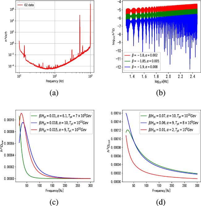
Figure 1. (a) presents the spectral energy density (h2Ω) of typical O2 data; (b) presents typical spectral energy density (h2Ω) of RGWinfl; (c) demonstrates the spectral energy density (h2Ω) of GWs originating from the sound waves for various parameters; (d) demonstrates some example spectral energy density (h2Ω) of GWs originating from the bubble collisions. The duration for this figure is one second. The vertical axis of (c), (d) is h2Ω. . |
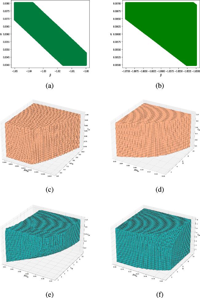
Table 2. Parameter settings for RGWinfl and the mean value (of p-value) for the confidence of the presence of such GW signals in real LIGO data (O2, O3a and O3b). The ‘Recognition accuracy’ is for the constructed CNN in determining whether the test data is mixed with the simulated GW signals. |
| Set | Parameter boundary | Magnitude of h2ΩGW | $\sqrt{PSD}$ (Hz−1/2) | Recognition accuracy | Mean p-value for O2 data plus simulated GW signals | Mean p-value (O2) | Mean p-value (O3a) | Mean p-value (O3b) |
|---|---|---|---|---|---|---|---|---|
| 1 | β ∈ (−1.85, −1.8) | ∼10−4 | ∼10−22 | 0.9982 | 0.99986713 | 0.00776 | 3.15 × 10⁻⁷ | 3.37 × 10⁻⁵ |
| α ∈ (0.004, 0.008) | ||||||||
| | ||||||||
| 2 | β ∈ (−1.87, −1.85) | ∼10−5 | ∼10−23 | 0.9422 | 0.9033364 | 0.10817 | 0.0035649 | 0.0005467 |
| α ∈ (0.005, 0.007) | ||||||||
| | ||||||||
| 3 | β ∈ (−1.91, −1.88) | ∼10−6 | ∼10−24 | 0.4961 | 0.501124 | 0.498391 | 0.4884417 | 0.487882 |
| α ∈ (0.006, 0.008) | (Unrecognized) | |||||||
| | ||||||||
| 4 | β ∈ (−2.0, −1.92) | ∼10−7 to | ∼10−25 to | 0.4917 | 0.5022312 | 0.500165 | 0.498763 | 0.489765 |
| α ∈ (0.007, 0.008) | ∼10−10 | ∼10−28 | (Unrecognized) | |||||
Table 3. Parameter settings for the GWs from FOPT and the mean p-value for the confidence of the presence of these GW signals in real LIGO data (O2, O3a and O3b). |
| GWs originating from sound waves | ||||||||
|---|---|---|---|---|---|---|---|---|
| Set | Parameter boundary | Magnitude of h2ΩGW | $\sqrt{PSD}$ (Hz−1/2) | Recognition accuracy | Mean p-value for O2 data plus simulated GW signals | Mean p-value (O2) | Mean p-value (O3a) | Mean p-value (O3b) |
| 1 | β/Hpt ∈ (0.01, 0.019) | ∼10−4 | ∼10−22 | 0.9994 | 0.994755 | 0.02574 | 4 × 10⁻⁶ | 1 × 10⁻⁴ |
| α ∈ (6.1, 10) | ||||||||
| Tpt ∈ (7 × 10⁹, 1010)Gev | ||||||||
| | ||||||||
| 2 | β/Hpt ∈ (0.02, 0.16) | ∼10−5 | ∼10−23 | 0.9494 | 0.94873 | 0.12302 | 0.00151 | 0.00058 |
| α ∈ (1, 10) | ||||||||
| Tpt ∈ (5 × 10⁹, 1010)Gev | ||||||||
| | ||||||||
| 3 | β/Hpt ∈ (0.17, 0.4) | ∼10−6 | ∼10−24 | 0.5012 | 0.499987 | 0.49341 | 0.48976 | 0.48875 |
| α ∈ (1.1, 10) | (Unrecognized) | |||||||
| Tpt ∈ (5 × 10⁸, 1010)Gev | ||||||||
| | ||||||||
| GWs originating from bubble collisions | ||||||||
| | ||||||||
| 4 | β/Hpt ∈ (0.01, 0.07) | ∼10−4 | ∼10−22 | 0.9998 | 0.999396 | 0.002406 | 6 × 10⁻⁵ | 1 × 10⁻⁵ |
| α ∈ (2, 10) | ||||||||
| Tpt ∈ (109, 1010)Gev | ||||||||
| | ||||||||
| 5 | β/Hpt ∈ (0.08, 0.2) | ∼10−5 | ∼10−23 | 0.9683 | 0.968897 | 0.062567 | 0.002691 | 0.001658 |
| α ∈ (1, 10) | ||||||||
| Tpt ∈ (5 × 10⁹, 8 × 10¹⁰)Gev | ||||||||
| | ||||||||
| 6 | β/Hpt ∈ (0.3, 0.7) | ∼10−6 | ∼10−24 | 0.4992 | 0.50231 | 0.49654 | 0.49002 | 0.48532 |
| α ∈ (4, 10) | (Unrecognized) | |||||||
| Tpt ∈ (2 × 10⁸, 1010)Gev | ||||||||
3. Estimation of likelihood of the presence of the targeted GW signals in real LIGO data by CNN
We construct a suitable one-dimensional CNN model, using the alternation of convolutional layers and pooling layers to extract the features of the samples. The structure of the CNN model is shown in table 1. Before training, we normalize the sample data to a range between 0 and 1, and set up by using ReLU [86] as the activation function, using Categorical Cross-Entropy (CCE) loss function to evaluate the deviation between the predicted values and the actual values, using Adam optimizer [87–89] to optimize the weights and biases of the CNN, and by setting the learning rate to 10−5. Finally, we employ the binary output score s of the network to calculate the confidence that the GW signal is present in the LIGO data through the softmax function [59]: 2 ), then we train CNNs for signals of each orders of magnitude separately. In each parameter space for the trained CNN model, we calculate the confidence that the real LIGO data (based on the 6000 raw sample obtained by O2, O3a and O3b data, respectively) contains the aforementioned three types of potential RGW signals, and the distributions and mean values are given. Tables 2 and 3, respectively, show the parameter space of the three GW models that we consider, and corresponding mean values of the confidence or likelihood.
$\begin{eqnarray}p=\frac{1}{1+{{\rm{e}}}^{-s}}.\end{eqnarray}$
The p-value ranges from 0 to 1 and we adopt it to characterize the confidence that the LIGO data contains these typical RGW signals. In this study, we use 0.5 as the threshold, and the closer the p-value is to 1, the higher the likelihood of the presence of targeted GW signals. In our analysis, we first generate simulated GW signals of different orders of magnitude across various parameter spaces (as mentioned in the section For the adjustment and adaptation processes, we initiated the construction of a CNN model with multiple convolutional layers and pooling layers, evaluating potential overfitting or underfitting by monitoring accuracy during training and testing as the epochs progressed. In cases of overfitting, we simplified the network structure by removing certain convolutional and pooling layers, whereas underfitting prompted the addition of layers to enhance the network’s complexity. Typically, we set the learning rate in the range of 10−3 to 10−5, recognizing that excessively high learning rates could compromise optimal training results. To address the overfitting, we also implemented the dropout technique to deactivate specific neurons, making the network more concise with enhanced efficiency. Through these adjustments, we successfully developed neural networks that have overcome the overfitting and underfitting challenges, enabling the CNNs to perform effectively on both training and test sets, achieving an optimal state.
From set 1 and 2 in table 2 and figures 3(a) and (b), we can see that when the parameter spaces of RGWinfl are [β ∈ (−1.85, −1.8), α ∈ (0.004, 0.008)] and [β ∈ ( −1.87, −1.85), α ∈ (0.005, 0.007)], the magnitude of spectral energy density of RGWinfl is ∼10−4 and ∼10−5; the recognition accuracy (the accuracy of the built CNN in determining whether the test data is mixed with the simulated GW signals, in addition to the real LIGO data) of the constructed CNN is around 0.99; the distributions of the confidence of containing RGWs in the 6000 samples from the O2, O3a and O3b data are less than 0.5, or, we found no evidence of presence of these RGWs. From set 3 in table 2 and figure 3(d), we can see that when the parameter space of the RGWs is [β ∈ (−1.91, −1.88), α ∈ (0.006, 0.008)], the magnitude of the spectral energy density of RGWs is ∼10−6; the recognition accuracy of the built CNN is around 0.49; some of the 6000 sample data in O2, O3a and O3b seem to contain RGW signals with confidence greater than 0.5, but we find that this is just due to the false positives (the reason is due to the invalidation of recognition for the GW signal parameters, this will be explained later).
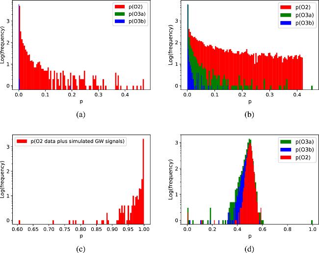
Figure 3. (a), (b) and (d) show the distribution of the confidence of containing typical targeted RGWs in the O2, O3a and O3b data for sets 1, 2 and 3 in table 2, respectively. The red, green and blue lines represent the distribution of the confidence of containing RGWs in the 6000 samples from the O2, O3a and O3b data, respectively. (c) illustrates the distribution of the confidence of containing simulated RGWs in the O2 data for set 1 in table 2. The x-axis represents the distribution of p-values; the y-axis represents the Log distribution frequency, i.e., we divided the distribution of p-value of 6000 samples into 100 narrow intervals, and count the number of samples with p-value sitting in each interval. |
From set 1 and 2 in table 3 and figures 4(a) and (b), we can see that for GWs from FOPT (sound wave case), where the parameter spaces of the GWs are [β/Hpt ∈ (0.01, 0.019), α ∈ (6.1, 10), Tpt ∈ (7 × 10⁹, 1010) Gev] and [β/Hpt ∈ (0.02, 0.16), α ∈ (1, 10), Tpt ∈ (5 × 10⁹, 1010) Gev], the magnitude of the spectral energy density of GWs is ∼10−4 and ∼10−5; the recognition accuracy of the built CNN is around 0.99; the distributions of confidence of the containing GWs in the 6000 samples from the O2, O3a and O3b data are less than 0.5, or , we found no evidence of the presence of such GW signals in the O2, O3a or O3b data. From set 4 and 5 in table 3 and figures 4(c) and (d), when GWs originated from the bubble collisions, where the parameter spaces of GWs are [β/Hpt ∈ (0.01, 0.07), α ∈ (2, 10), Tpt ∈ (109, 1010) Gev] and [β/Hpt ∈ (0.08, 0.2), α ∈ (1, 10), Tpt ∈ (5 × 10⁹, 8 × 10¹⁰) Gev], the magnitude of spectral energy density of GWs is ∼10−4 and ∼10−5; the recognition accuracy of established CNN is close to 0.99; the confidences is less than 0.5, thereby finding no evidence of the presence of such GW signals in the data from O2, O3a or O3b.
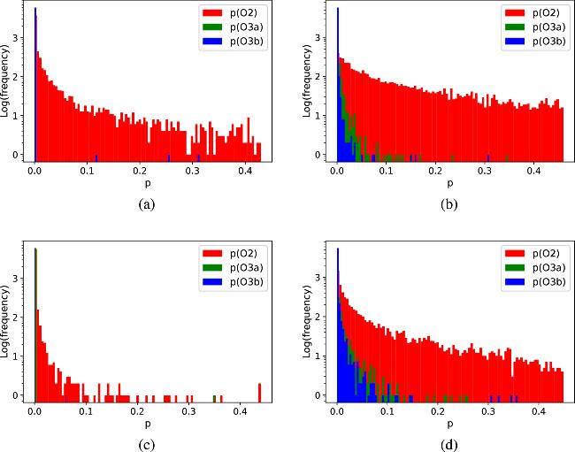
Figure 4. (a), (b), (c) and (d) demonstrate the distributions of the confidence of containing the GWs from FOPT in the O2, O3a and O3b data for sets 1, 2, 4 and 5 in table 3, respectively. The red, green and blue lines represent the distribution of the confidence of containing the GWs from FOPT in the 6000 samples from the O2, O3a and O3b data, respectively. The y-axis represents the Log distribution frequency. |
Next, we use constructed CNN (table 1) to estimate the parameters of GW signals. The purpose of this task is to check whether the networks we establish really have sufficiently acquired the ability to recognize the features and parameters of the signals. We consider three GW models of equations (4 ), (5 ) and (8 ), respectively. For each type of GW model, within the parameter spaces, we obtained a total of 100,000 O2 data samples containing simulated GW signals. We use the mean squared error (MSE) loss function to evaluate the deviation between the predicted and true values. In the final layer, we use the linear activation function to output the predicted values. From figures 5(a) (b) and 6, it is evident that our network model can recognize the characteristics of GW signals by correctly estimating their corresponding multiple parameters. As mentioned earlier, the selected sample points can cover the parameter regions corresponding to each order of magnitude of the GW signals. Moreover, for dividing the training and testing sets, we also follow the principle of random distribution. Therefore, our network can reliably and robustly identify these GW signals in specific orders of magnitude within the parameter regions. This ability is based on the confirmed capability of the network to recognize these concrete parameters, rather than relying on other arbitrary criteria or simply distinguishing between the presence or absence of any unknown signals. For example, as shown in table 3 (line 5), the model exhibits a very high recognition accuracy, so if any GW signal within the corresponding parameter region appears, we have reason to believe in its presence. If the test on the real LIGO data yields a null result, such an output is also reliable, at least for the region of parameters we are concerned with. In contrast, the results shown in figures 5(c) and (d) indicate that for the order of magnitude (∼10−6) of RGWinfl signals, the built CNN has no ability to correctly recognize the characteristics of the RGWinfl signals, or, their parameters cannot be properly estimated, and this is also the reason for the false positive in figure 3(d). Here, please also notice that, the parameter ranges in figure 5 are small, and such ranges are also calculated by the reverse mapping process mentioned above. For instance, in figure 2(a) we can find the range of α from 0.004 to 0.008, the same as in figure 5(b), corresponding to h2ΩGW ∼ 10−4, which can also be found consistently in table 2 (set 1). It is the same for parameter β in figure 5.
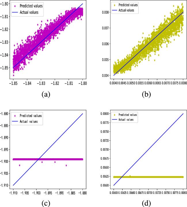
Figure 5. (a) and (b) express the results of simultaneous estimation of GW parameters β and α for 10000 samples in set 1 of table 2. Here β ∈ (−1.85, −1.8), α ∈ (0.004, 0.008). The residuals are 0.00071 and 0.00025, respectively. (c) and (d) display the results of simultaneous estimation of β and α for 10000 samples in set 3 of table 2. Here β ∈ (−1.91, −1.88), α ∈ (0.006, 0.008). Importantly, the results shown in (c) and (d) indicate that for such order of magnitude of GW signals, the built CNN cannot correctly recognize or estimate corresponding GW parameters, so in such case the p-value given by the CNN is not reliable, and this is also the reason for the false positive in (d) of figure 3. |
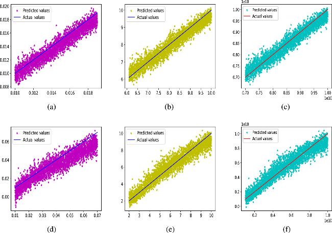
Figure 6. (a), (b) and (c) demonstrate the results of simultaneous estimation of parameters β/Hpt, α and Tpt for 10000 samples in set 1 of table 3. Here β/Hpt ∈ (0.01, 0.019), α ∈ (6.1, 10), Tpt ∈ (7 × 10⁹, 1010)Gev. The residuals are 0.000148, 0.0354 and 0.01026, respectively. (c), (d) and (e) show the results of simultaneous estimation of parameters β/Hpt, α and Tpt for 10000 samples in set 4 of table 3. Here β/Hpt ∈ (0.01, 0.07), α ∈ (2, 10), Tpt ∈ (109, 1010)Gev. The residuals are 0.00498, 0.01611 and 0.00148, respectively. The solid lines represent the actual values, and the dots represent the predicted values; these parameters are correctly estimated for the above cases. |
In traditional methods used to constrain GWs, some noises are uncorrelated between different detectors, so utilizing the cross-correlation relationship between two detectors helps achieve higher sensitivity usually by several orders of magnitude, and such correlation can be quantified by the overlap reduction function [90, 91] (a dimensionless function of frequency encoding relative locations and orientations of GW detector pair), and these topics have been extensively investigated in previous studies like [90–107]. Particularly, focusing on the SGWB, the LIGO Scientific Collaboration, Virgo Collaboration and KAGRA Collaboration, reported a series of results by use of cross-correlation (overlap reduction function) for the O1, O2 and O3 runs. For example, in 2017, the [98] for O1 provided Ω0 < 1.7 × 10⁻⁷, and comparatively, our result in this article, the h2ΩGW is in the level of 10−5 (see tables 2 and 3; the ‘h’ is the reduced Hubble parameter with a value of about 0.6). Later, in the 2018 paper [99] and 2019 paper [102] for O1 and O2, the reported sensitivities gradually increased, and in the 2021 paper [104] for O3, the upper limit of ΩGW was suppressed into 10−9. These results (giving lower upper limits) are more accurate than what we obtain by the CNN here, and this is mainly due to the limitations of the current structure of the neural network that we use, e.g., not benefited by the cross-correlation relationship. However, through our study as an exploration, we have recognized how to ensure the reliability of the results produced by the aforementioned deep learning neural networks, e.g., as shown in figure 5, when the GW parameters can be correctly recognized and estimated for specific GW strengths, the obtained high p-value and corresponding upper limit are reliable and adoptable. Thus, holding such premises and guidelines, we will endeavor to develop more advanced CNN architectures or more complex neural networks, such as those leveraging the cross-correlation, to achieve enhanced sensitivity and improved upper limits in the future. These anticipated efforts involve massive computation and fundamental modifications, and we shall try to pursue such studies in subsequent works.
4. Conclusion and discussion
In this work, we search for typical RGWs (from the early stages of the Universe as key components of SGWB) in the real LIGO data. Our focus is primarily on RGWs from the inflation and the FOPT (by sound waves and bubble collisions). By adjustment and adaptation processes, we successfully establish effective and targeted deep learning neural networks to calculate the likelihood of the presence of the above RGWs in the real LIGO data. Additionally, we attempt to estimate their relevant parameters and provide constraints on strengths of these RGWs. We find the following results:
1. When the parameter region of RGWinfl are within [β ∈ (−1.85, −1.8), α ∈ (0.004, 0.008)] and [β ∈ (−1.87, −1.85), α ∈ (0.005, 0.007)] (the corresponding magnitudes of the spectral energy density of RGWinfl are ∼10−4 and ∼10−5), the distributions of the confidence of containing RGWinfl in the 6000 samples from the real LIGO data O2, O3a and O3b is less than 0.5, or, we found no evidence of the presence of RGWinfl signals in these data. When the parameter region of RGWinfl are within [β ∈ (−1.91, −1.88), α ∈ (0.006, 0.008)] (the corresponding magnitude of spectral energy density of RGWinfl is ∼10−6), some of the 6000 sample data in O2, O3a and O3b seem to contain RGW signals with confidence greater than 0.5; however, this result is due to the false positive, explained in section 3 , (also see figure 5), that, when the constructed CNN cannot correctly estimate the parameters of the predicted GWs, the given p-value is not reliable or adoptable.
2. For the GWs from FOPT (sound wave case), with the parameter region within [β/Hpt ∈ (0.01, 0.019), α ∈ (6.1, 10), Tpt ∈ (7 × 10⁹, 1010) Gev] and [β/Hpt ∈ (0.02, 0.16), α ∈ (1, 10), Tpt ∈ (5 × 10⁹, 1010) Gev] (the corresponding magnitudes of spectral energy density of GWs are ∼10−4 and ∼10−5), the distributions of the confidence of containing GWs in the 6000 samples from the real LIGO data O2, O3a and O3b are less than 0.5, or, we found no evidence of the presence of such GW signals in this data. For the case of GWs from the bubble collisions, for the parameter region within [β/Hpt ∈ (0.01, 0.07), α ∈ (2, 10), Tpt ∈ (109, 1010) Gev] and [β/Hpt ∈ (0.08, 0.2), α ∈ (1, 10), Tpt ∈ (5 × 10⁹, 8 × 10¹⁰) Gev] (the corresponding magnitudes of spectral energy density of the GWs are ∼10−4 and ∼10−5), the distributions of the confidence of containing such GWs in the 6000 samples from the real LIGO data O2, O3a and O3b are also less than 0.5, or, the same, we found no evidence of their presence.
In fact, deep neural networks may result in misclassifications by failing to capture certain features of the signals, due to their limited generalization ability. However, in this paper, the selected sample points cover the corresponding parameter regions for different orders of magnitude, thereby minimizing potential omissions. Furthermore, the neural network’s binary classification decisions may also be affected by the presence of other false signals. However, through parameter estimation, we observe that the model possesses excellent capabilities for parameter recognition. In other words, these abilities rely on accurate estimations of specific parameters, thereby avoiding other false signals to be identified as true signals (as also described in the final part of section 3 ). For instance, when the GW parameters can be correctly recognized and estimated for cases with a specific order of magnitude of GW strengths [figure 5(a), (b) and figure 6], if the simulated GW signals are included in the test data, the established CNN consistently gives very high ‘recognition accuracy’ and very high p-value [see sets 1 and 2 of table 2, and sets 1, 2, 4 and 5 of table 3, and figure 3(c)]. Thus, if the given p-value is low, it is believable that there is no presence of the targeted GWs. Conversely, when the GW parameters cannot be correctly estimated for cases with certain GW strengths [e.g. Figure 5(c) and (d)], even if the test data does contain the simulated GW signals, the CNN gives low recognition accuracy and low p-value (e.g. set 3 of table 2). For this situation, even if the CNN gives p-values greater than the threshold of 0.5 after testing some data [e.g. Figure 3(d)], this still does not serve as adoptable evidence for the presence of such GW signals (treated as false positive). Therefore, based on the above considerations and operations, we suggest that the acquired results in this work are reliable.
Briefly, the results indicate no evidence of the presence of the targeted GWs from 1) inflation, 2) sound waves, or 3) bubble collisions, predicted by typical models. For these three cases, the results provide upper limits of their GW spectral energy densities, respectively as: 1) h2ΩGW ∼ 10−5 [correspondingly in a 2D parameter region within boundary of β ∈ (−1.87, −1.85) × α ∈ (0.005, 0.007)], and 2) h2ΩGW ∼10−5 [in a 3D parameter region within a boundary of β/Hpt ∈ (0.02, 0.16) × α ∈ (1, 10) × Tpt ∈ (5 × 10⁹, 1010) Gev], and 3) h2ΩGW ∼10−5 [in a 3D parameter region within a boundary of β/Hpt ∈ (0.08, 0.2) × α ∈ (1, 10) × Tpt ∈ (5 × 10⁹, 8 × 10¹⁰) Gev]. Although only null results and upper limits are obtained here, our analysis suggests that the above methods and neural networks are effective and reliable, which can be applied not only for the current data but also for the upcoming O4 data. Furthermore, we will endeavor to develop more advanced CNN architectures or more complex neural networks, such as those leveraging cross-correlation, to achieve enhanced sensitivity and refined upper limits in the future, to explore possible RGWs from the early stages of the Universe or provide constraints on relevant cosmological theories. These efforts will be pursued in subsequent works.