


1. Introduction
The amplification mechanism of an optical beam (the master laser) injected through the cavity of a slave laser has been extensively reported in both below and above-threshold states by numerous physicists [1–4]. The above-threshold state is further divided into two distinct regimes of single and multiple-frequency [5–7]. The multiple-frequency regime includes many signal and image satellite lines produced by the four-wave mixing interaction between the amplified input signal and the strong cavity electric field [8, 9]. By increasing the intensity or reducing the frequency detuning of the input signal at the boundary of these two regimes, the injection-locking phenomenon happens suddenly, so that the cavity electric field, together with the signal and image satellite lines, are simultaneously captured by the input signal [8, 10]. Therefore, the below-threshold state and the injection-locked regime of a laser amplifier exactly mimic the above-threshold state of a free-running laser due to a single-component cavity electric field that oscillates at the input signal rather than cavity resonance frequency [2, 11].
The noise aspect of laser amplifiers has usually been studied by solving the Maxwell–Bloch equations of motion in the simultaneous presence of two fluctuating Langevin forces of the atomic population inversion ${{\rm{\Gamma }}}_{D}$ and atomic dipole moment ${{\rm{\Gamma }}}_{d}$ [12–14]. The third one is the cavity Langevin force ${{\rm{\Gamma }}}_{\alpha }$ which has always been ignored due to the negligible number of thermal photons inside the laser cavity [12, 13]. However, the first contradictory proof was published in 2012 where the Maxwell–Bloch equations of motion were solved in the presence of cavity Langevin force alone [15]. It was demonstrated that the cavity Langevin force is not only negligible but it can also generate the different noise spectra of a single-peak Lorentzian profile for the class-A lasers [15] and a double-peak profile for the class -B lasers [16] in complete agreement with the experimental and theoretical results [10, 13].
Recently, the Maxwell–Bloch equations of motion have been widely used to describe the behavior of various physical systems such as the effect of photon propagation on a near-zero-refractive-index medium [17], terahertz (THz) frequency quantum cascade lasers (QCLs) [18], localized gap modes of coherently trapped atoms in an optical lattice [19], generation of optical pulses by locking of laser longitudinal modes [20], stochastic Maxwell–Bloch equations for modeling amplified spontaneous emission [21], and so on [22–24].
The present paper aims to reveal the significance of cavity Langevin force by extending previous noise calculations from the simple case of a free-running laser [15] to the more complicated case of a class-A laser amplifier. The input signal is considered an ideal coherent light with a fixed amplitude and phase (no fluctuation) which is injected into the free-running laser cavity for amplification. However, it is observed that the amplitude and phase of the output amplified signal along with the static atomic population inversion seriously suffer from the fluctuations imposed by the laser pumping system [25–27]. Therefore, a key objective is to identify these fluctuations and their corresponding noise fluxes by solving the laser amplifier equations of motion in the presence of cavity Langevin force. It is demonstrated that the input noise flux of pumping supplies the output noise fluxes of amplitude and spontaneous emission according to the flux conservation law.
The next priority is to specify the coherence time of light emitted from the laser amplifier in terms of the parameters of the laser and input signal [28]. The degree of first-order temporal coherence (DFOTC) is then determined by taking the correlation function of the amplitude fluctuations of the cavity electric field in the time domain. The damping rate of DFOTC displays a reverse relation with the coherent time, but a direct relation with the identical bandwidths of amplitude and spontaneous emission noise fluxes [29]. Meanwhile, these dependent quantities are calculated as a function of the amplitude and frequency detuning of the input signal, the laser pumping rate, and the mean cavity damping rate. For instance, suppose one measures the coherence time by an interferometer setup [28, 29], the other dependent optical variables including DFOTC, noise fluxes, and their bandwidths can be calculated by the relations provided in this manuscript without any measurement. The noise fluxes of free-running class-A laser are directly extracted from those of class-A laser amplifiers by ignoring the amplitude and frequency detuning of the input signal. Finally, the bandwidth of amplitude noise flux and the coherence time have been changed, reversely, by increasing the laser pumping rate from the below to the above-threshold state.
The manuscript is organized into the following sections. Section 1 provides an introduction to the project and outlines its objectives. Section 2 presents the motion equations of the class-A laser amplifier, along with the zero-order and first-order solutions. In section 3 , we calculate the output noise flux, which includes the contributions from amplitude and spontaneous emission noise fluxes, as well as the input noise flux generated by the pumping system. It is then demonstrated that these noise fluxes conform to the principle of flux conservation. Section 4 focuses on the noise fluxes of the free-running laser, which are derived from the noise fluxes of the laser amplifier by ignoring the input signal parameters. In section 5 , we define the DFOTC, coherence time, and their relationships with the amplitude noise flux for the laser amplifier. Section 6 provides the same information for the free-running laser. Finally, the results are discussed in the conclusion presented in section 7 .
2. The motion equations and trial solutions
The general feature of class-A laser amplifiers is described by the two motion equations of Maxwell–Bloch in the forms [13, 15, 30, 31]
$\begin{eqnarray}\dot{\alpha }\,+\,\left({\gamma }_{C}+{\rm{i}}{\omega }_{L}\right)\,\,\alpha =\displaystyle \frac{{g}^{2}}{{\gamma }_{\perp }}\,\alpha \,D+{{\rm{\Gamma }}}_{\alpha }+{\gamma }_{2}^{1/2}{\beta }_{{\rm{in}}},\end{eqnarray}$
and $\begin{eqnarray}{\gamma }_{| | }D={\gamma }_{| | }{D}_{P}-\displaystyle \frac{2{g}^{2}}{{\gamma }_{\perp }}\,{\left|\alpha \right|}^{2}D,\end{eqnarray}$
where the variables $\alpha $ and $D$ are the cavity electric field and atomic population inversion with the respective damping rates ${\gamma }_{C}$ and ${\gamma }_{| | }$. ${\gamma }_{\perp }$ is the damping rate of atomic dipole moment whose equation of motion has adiabatically been eliminated due to the damping condition ${\gamma }_{\perp }\gg {\gamma }_{| | }\gg {\gamma }_{C}$ of class-A lasers. ${\gamma }_{| | }{D}_{P}$ is the laser pumping rate whose energy is partially converted to the spontaneous emission radiation by the rate ${\gamma }_{| | }D$. The cavity resonance frequency and coupling constant between the cavity electric field and atomic dipole moment are denoted by ${\omega }_{L}$ and $g$, respectively. The cavity Langevin force is displayed by ${{\rm{\Gamma }}}_{\alpha }$ with a zero-mean value $\langle {{\rm{\Gamma }}}_{\alpha }\rangle \,=0$ and the following correlation function [15] $\begin{eqnarray}\begin{array}{l}\langle {{\rm{\Gamma }}}_{\alpha }(\omega )\,{{\rm{\Gamma }}}_{\alpha }^{\ast }(\omega ^{\prime} \,)\,\rangle \\ \,=\,2\,{\gamma }_{C}\,({n}_{{\rm{th}}}+1)\,\,\delta \,(\omega -\omega ^{\prime} )\,\approx 2\,{\gamma }_{C}\,\delta \,(\omega -\omega ^{\prime} ),\end{array}\end{eqnarray}$
where the correlation function relation $\langle {{\rm{\Gamma }}}_{\alpha }^{\ast }\,(\omega ^{\prime} ){{\rm{\Gamma }}}_{\alpha }\,(\omega )\,\rangle \,=2\,{\gamma }_{C}\,{n}_{{\rm{th}}}\,\delta \,(\omega -\omega ^{\prime} )$ is ignored due to the negligible number of thermal photons ($n{}_{{\rm{th}}}\ll 1$) inside the laser cavity [15, 16]. Finally, the input signal ${\beta }_{{\rm{in}}}$ is injected through one of the cavity mirrors with the amplitude loss rate ${\gamma }_{2}^{1/2}$ for amplification. It is characterized by the two key parameters of amplitude ${\beta }_{S}$ and frequency detuning ${\omega }_{d}={\omega }_{S}-{\omega }_{L}$, where $S\ne L$, in the form $\begin{eqnarray}\begin{array}{l}{\beta }_{{\rm{in}}}={\beta }_{S}\exp (-{\rm{i}}\,{\omega }_{S}t)\\ \,=\,{\beta }_{S}\exp [-{\rm{i}}\,({\omega }_{L}+{\omega }_{d})t].\end{array}\end{eqnarray}$
The single-mode cavity electric field $\alpha (t)$ and the atomic population inversion $D(t)$ have been presented here in the general forms
$\begin{eqnarray}\alpha (t)=\left[{\alpha }_{S}+\delta {\alpha }_{S}(t)\right]\exp [-{\rm{i}}\,({\omega }_{L}+{\omega }_{d})t+{\rm{i}}\delta {\varphi }_{S}(t)],\end{eqnarray}$
and $\begin{eqnarray}D(t)={D}_{S}+\delta {D}_{S}(t),\end{eqnarray}$
where ${\alpha }_{S}$ and ${D}_{S}$ are, respectively, the amplitude of the cavity electric field and the statics atomic population inversion which fluctuated by the real values $\delta {\alpha }_{S}(t)$ and $\delta {D}_{S}(t)$ due to the cavity Langevin (fluctuating) force ${{\rm{\Gamma }}}_{\alpha }$. $\delta {\varphi }_{S}(t)$ is the third real fluctuating variable associated with the phase of the cavity electric field.By substituting the trial solutions (4 )-(6 ) into the Maxwell–Bloch equations of motion (1 ) and (2 ), a cubic equation is turned out for the normalized mean number of photons ${\left|{\alpha }_{S}\right|}^{2}/{n}_{S}$ inside the laser cavity correct to the zero-order fluctuation ($\delta {\alpha }_{S}\approx \delta {D}_{S}\approx \delta {\varphi }_{S}\approx 0$ ) as [32]7 ) into the following relation [8]
$\begin{eqnarray}\begin{array}{c}\left[1+{\left({\omega }_{d}/{\gamma }_{C}\right)}^{2}\right]\,{\left(\displaystyle \frac{{\left|{\alpha }_{S}\right|}^{2}}{{n}_{S}}\right)}^{3}+\left[2\,(1-C)+2\,{\left({\omega }_{d}/{\gamma }_{C}\right)}^{2}\right.\\ \left.-\,\left(\displaystyle \frac{{\gamma }_{2}}{{\gamma }_{C}}\right)\displaystyle \frac{\,{\left|{\beta }_{S}\right|}^{2}}{{\gamma }_{C}\,{n}_{S}}\right]\,{\left(\displaystyle \frac{{\left|{\alpha }_{S}\right|}^{2}}{{n}_{S}}\right)}^{2}+\left[{(1-C)}^{2}+{\left({\omega }_{d}/{\gamma }_{C}\right)}^{2}\right.\\ \left.-\,2\,\left(\displaystyle \frac{{\gamma }_{2}}{{\gamma }_{C}}\right)\displaystyle \frac{\,{\left|{\beta }_{S}\right|}^{2}}{{\gamma }_{C}\,{n}_{S}}\right]\displaystyle \frac{{\left|{\alpha }_{S}\right|}^{2}}{{n}_{S}}-\left(\displaystyle \frac{{\gamma }_{2}}{{\gamma }_{C}}\right)\displaystyle \frac{\,{\left|{\beta }_{S}\right|}^{2}}{{\gamma }_{C}\,{n}_{S}}\,=\,0,\end{array}\end{eqnarray}$
where the normalized pumping rate $C={\gamma }_{| | }{D}_{P}/{\gamma }_{| | }{D}_{0}$ has a value less than one in the below-threshold state ($C\lt 1$), equal to one at the threshold state ($C=1$), and larger than one in the above-threshold state ($C\gt 1$). ${D}_{0}={\gamma }_{\perp }{\gamma }_{C}/{g}^{2}$ is the statics population inversion in the above-threshold state of the free-running laser, and ${n}_{S}={\gamma }_{\perp }{\gamma }_{| | }/2{g}^{2}$ is the number of cavity photons in the saturation state at the normalized pumping rate $C=2$ [8, 13]. The normalized population inversion of the laser amplifier ${D}_{S}/{D}_{0}$ is then calculated by substituting the numerical solutions of ${\left|{\alpha }_{S}\right|}^{2}/{n}_{S}$ from the cubic equation ( $\begin{eqnarray}\displaystyle \frac{{D}_{S}}{{D}_{0}}=\displaystyle \frac{C}{1+{\left|{\alpha }_{S}\right|}^{2}/{n}_{s}}.\end{eqnarray}$
On the other side, the motion equations for the three fluctuating variables $\delta {\alpha }_{S}$, $\delta {D}_{S}$, and $\delta {\varphi }_{S}$ are similarly derived by substituting the trial solutions (4 )-(6 ) into the Maxwell–Bloch equations of motion (1 ) and (2 ), but by considering the terms correct to the first-order fluctuation ($\delta {\alpha }_{S}^{2}\approx \delta {D}_{S}^{2}\approx \delta {\varphi }_{S}^{2}\approx 0$) as9 ), it is separated into the real and imaginary parts in the frequency domain as10 )–(12 ) in the forms3 . Meanwhile, the singularity condition ${\gamma }_{C}B={\rm{i}}\omega $ does not occur in equations (13 )–(15 ) because substituting equation (8 ) into equation (16 ) fails to yield a real value for the mean number of photons ${\left|{\alpha }_{S}\right|}^{2}/{n}_{S}$ when solving the equation ${\gamma }_{C}B={\rm{i}}\omega $.
$\begin{eqnarray}\begin{array}{c}\delta {\dot{\alpha }}_{S}+{\rm{i}}\left|{\alpha }_{S}\right|\delta {\dot{\varnothing }}_{S}\\ +\,{\gamma }_{C}\left(1-\displaystyle \frac{{D}_{S}}{{D}_{0}}-{\rm{i}}\displaystyle \frac{{\omega }_{d}}{{\gamma }_{C}}\right)\delta {\alpha }_{S}-\,\displaystyle \frac{{g}^{2}}{{\gamma }_{\perp }}\left|{\alpha }_{S}\right|\delta {D}_{S}\\ =\,{{\rm{\Gamma }}}_{\alpha }\exp \left({\rm{i}}{\omega }_{s}t-{\rm{i}}\delta {\phi }_{S}\right),\end{array}\end{eqnarray}$
and $\begin{eqnarray}{\gamma }_{| | }\,{\left(1+\displaystyle \frac{{\left|{\alpha }_{S}\right|}^{2}}{{n}_{S}}\right)}^{2}\delta {D}_{S}=-4\,{\gamma }_{C}C\,\left|{\alpha }_{S}\right|\,\delta {\alpha }_{S}.\end{eqnarray}$
Now by taking the Fourier transform of equation ( $\begin{eqnarray}\begin{array}{l}-{\rm{i}}\omega \,\delta {\alpha }_{S}(\omega )+{\gamma }_{C}\left(1-\displaystyle \frac{{D}_{S}}{{D}_{0}}\right)\,\delta {\alpha }_{S}(\omega )-\displaystyle \frac{{g}^{2}}{{\gamma }_{\perp }}\left|{\alpha }_{S}\right|\delta {D}_{S}(\omega )\\ \,=\,\displaystyle \frac{1}{2}\,\left[{{\rm{\Gamma }}}_{\alpha }\left({\omega }_{S}+\omega \right)+{{\rm{\Gamma }}}_{\alpha }^{\ast }\left({\omega }_{S}+\omega \right)\right],\end{array}\end{eqnarray}$
and $\begin{eqnarray}\begin{array}{l}\omega \,\left|{\alpha }_{S}\right|\,\delta {\varphi }_{S}(\omega )-{\rm{i}}{\omega }_{d}\,\delta {\alpha }_{S}(\omega )\\ \,=\,\displaystyle \frac{1}{2}\,\left[{{\rm{\Gamma }}}_{\alpha }\left({\omega }_{S}+\omega \right)-{{\rm{\Gamma }}}_{\alpha }^{\ast }\left({\omega }_{S}+\omega \right)\right].\end{array}\end{eqnarray}$
The three variables $\delta {\alpha }_{S}(\omega )$, $\delta {\varphi }_{S}(\omega )$, and $\delta {D}_{S}(\omega )$ will ultimately be rendered from the simultaneous solution of equations ( $\begin{eqnarray}\delta {\alpha }_{S}(\omega )\,=\,\displaystyle \frac{{{\rm{\Gamma }}}_{\alpha }({\omega }_{S}+\omega )+{{\rm{\Gamma }}}_{\alpha }^{\ast }({\omega }_{S}+\omega )}{2\,\left({\gamma }_{C}B-{\rm{i}}\,\omega \right)},\end{eqnarray}$
$\begin{eqnarray}\begin{array}{c}\delta {\varphi }_{S}(\omega )\,=\,\displaystyle \frac{\left({\gamma }_{C}B-{\rm{i}}\,\omega \right)\,\left[{{\rm{\Gamma }}}_{\alpha }({\omega }_{S}+\omega )-{{\rm{\Gamma }}}_{\alpha }^{\ast }({\omega }_{S}+\omega )\right]\,+{\rm{i}}{\omega }_{d}\,\left[{{\rm{\Gamma }}}_{\alpha }({\omega }_{S}+\omega )+{{\rm{\Gamma }}}_{\alpha }^{\ast }({\omega }_{S}+\omega )\right]\,}{2\,\omega \,\left|{\alpha }_{S}\right|\,\left({\gamma }_{C}B-{\rm{i}}\,\omega \right)},\end{array}\end{eqnarray}$
and $\begin{eqnarray}\begin{array}{c}\delta {D}_{S}(\omega )=\,\displaystyle \frac{-2\,{\gamma }_{C}C\,\left|{\alpha }_{S}\right|\,\left[{{\rm{\Gamma }}}_{\alpha }({\omega }_{S}+\omega )+{{\rm{\Gamma }}}_{\alpha }^{\ast }({\omega }_{S}+\omega )\right]}{\,{\gamma }_{| | }\,\left({\gamma }_{C}B-{\rm{i}}\,\omega \right)\,{\left(1+{\left|{\alpha }_{S}\right|}^{2}/{n}_{S}\right)}^{\,2}},\end{array}\end{eqnarray}$
where $\begin{eqnarray}B=1-\displaystyle \frac{{D}_{S}}{{D}_{0}}\,+2\,{C}^{-1}\,\left(\displaystyle \frac{{\left|{\alpha }_{S}\right|}^{2}}{{n}_{S}}\right)\,{\left(\displaystyle \frac{{D}_{S}}{{D}_{0}}\right)}^{2},\end{eqnarray}$
is a dimensionless quantity so that 2B will represent the normalized common bandwidth of amplitude, spontaneous emission, and pumping noise fluxes in section 3. Balance between the noise fluxes of amplitude ${N}_{{\rm{AM}}}^{{\rm{LA}}}(\omega )$, spontaneous emission ${N}_{{\rm{SP}}}^{{\rm{LA}}}(\omega )$, and pumping ${N}_{{\rm{Pump}}}^{{\rm{LA}}}(\omega )$
Assume that $a\,(\omega )$ is an arbitrary fluctuating variable originating from white noise (Dirac function), then it is required to satisfy the following correlation function in a complex conjugate form [33]3 ), which is proportional to a Dirac function (white noise) with the diffusion coefficient $2\,{\gamma }_{C}$. Therefore, the solutions (13 )-(15 ) associated with the three fluctuating variables of the cavity electric field amplitude $\delta {\alpha }_{S}(\omega )$, phase $\delta {\varphi }_{S}(\omega )$, and atomic population inversion $\delta {D}_{S}(\omega )$ obey the correlation function equation (17 ).
$\begin{eqnarray}\langle {a}^{\ast }(\omega )\,a\,(\omega ^{\prime} \,)\rangle \,=\,2\pi \,h(\omega )\,{h}^{\ast }(\omega ^{\prime} \,)\,\delta (\omega -\omega ^{\prime} ),\end{eqnarray}$
where ${\left|h\,(\omega )\right|}^{2}$ represents the dimensionless mean flux per unit angular frequency bandwidth at angular frequency $\omega $. It is noteworthy that the cavity Langevin force ${{\rm{\Gamma }}}_{\alpha }$ generates various types of noise fluxes due to the correlation function relation (The amplitude noise flux within the laser cavity ${\left|{h}_{{\rm{AM}}}^{{\rm{LA}}}(\omega )\right|}^{2}$ is determined by substituting the fluctuating variable $\delta {\alpha }_{S}(\omega )$ from equation (13 ) into the correlation function equation (17 ). The amplitude noise flux of the laser amplifier ${N}_{{\rm{AM}}}^{{\rm{LA}}}(\omega )$, which emerges from the cavity mirrors of the total damping rate $2\,{\gamma }_{C}={\gamma }_{1}+{\gamma }_{2}$, is finally obtained in the form7 ) and the relation (8 ), respectively. It implies that the amplitude noise flux (18 ) and its normalized bandwidth (19 ) can be adjusted by changing three external parameters: the normalized input signal flux ${\left|{\beta }_{S}\right|}^{2}/{\gamma }_{C}{n}_{s}$, the frequency detuning ${\omega }_{d}/{\gamma }_{C}$, and the laser pumping rate $C$. In addition, the mean damping rate of cavity mirrors ${\gamma }_{C}$ plays a similar adjusting role through the normalized quantities of amplitude bandwidth ${({\rm{\Delta }}\omega )}_{{\rm{AM}}}^{{\rm{LA}}}/{\gamma }_{C}$, frequency detuning ${\omega }_{d}/{\gamma }_{C}$, and Fourier frequency $\omega /{\gamma }_{C}$.
$\begin{eqnarray}{N}_{{\rm{AM}}}^{{\rm{LA}}}(\omega )=2{\gamma }_{C}{\left|{h}_{{\rm{AM}}}^{{\rm{LA}}}(\omega )\right|}^{2}=\displaystyle \frac{{\gamma }_{C}^{2}}{2\pi \,\left({\omega }^{2}+{\gamma }_{C}^{2}{B}^{2}\right)},\end{eqnarray}$
where it has a Lorentzian profile with a normalized bandwidth equal to $\begin{eqnarray}\begin{array}{l}\displaystyle \frac{{\left({\rm{\Delta }}\omega \right)}_{{\rm{AM}}}^{{\rm{LA}}}}{{\gamma }_{C}}=2B\\ \,=\,2\,\left[1-\displaystyle \frac{{D}_{S}}{{D}_{0}}\,+2\,{C}^{-1}\,\left(\displaystyle \frac{{\left|{\alpha }_{S}\right|}^{2}}{{n}_{S}}\right)\,{\left(\displaystyle \frac{{D}_{S}}{{D}_{0}}\right)}^{2}\right].\end{array}\end{eqnarray}$
In this context, the superscript LA denotes the laser amplifier state, while the subscript AM refers to amplitude noise flux. It is important to note that the variables of ${\left|{\alpha }_{S}\right|}^{2}/{n}_{S}$ and ${D}_{S}/{D}_{0}$ are calculated numerically by using the cubic equation (The variations of amplitude noise flux ${N}_{{\rm{AM}}}^{{\rm{LA}}}(\omega )$ versus the normalized Fourier frequency $\omega /{\gamma }_{C}$ are illustrated in figure 1 for a symmetrical cavity ${\gamma }_{1}={\gamma }_{2}={\gamma }_{C}$, the typical normalized input signal flux ${\left|{\beta }_{S}\right|}^{2}/{\gamma }_{C}{n}_{s}=0.25$, the various values of normalized frequency detuning ${\omega }_{d}/{\gamma }_{C}=$ 0.25, 0.5, 0.75, and 1, and the normalized pumping rates (a) $C=0.5$ and (b) $C=1.2$ in the respective below-threshold and above-threshold states. As expected for a fixed value of normalized input light intensity ${\left|{\beta }_{S}\right|}^{2}/{\gamma }_{C}{n}_{s}$ and frequency detuning ${\omega }_{d}/{\gamma }_{C}$, a homogeneous broadening of the Lorentzian profile occurs for the light emerging from the laser amplifier cavity in the frequency domain $\omega $. The frequency broadening is caused by the temporal fluctuations in the number of photons passing through the cavity mirrors, and randomly scattered by phonons and atoms due to the diffusion coefficient $2{\gamma }_{C}$ in equation (3 ). The Lorentzian profiles observed in both below-threshold and above-threshold states align with the empirical results from laser amplifiers (refer to figure 3(b) in [10] and [27]) as well as free-running lasers (see figures 1 and 2 in [15]).
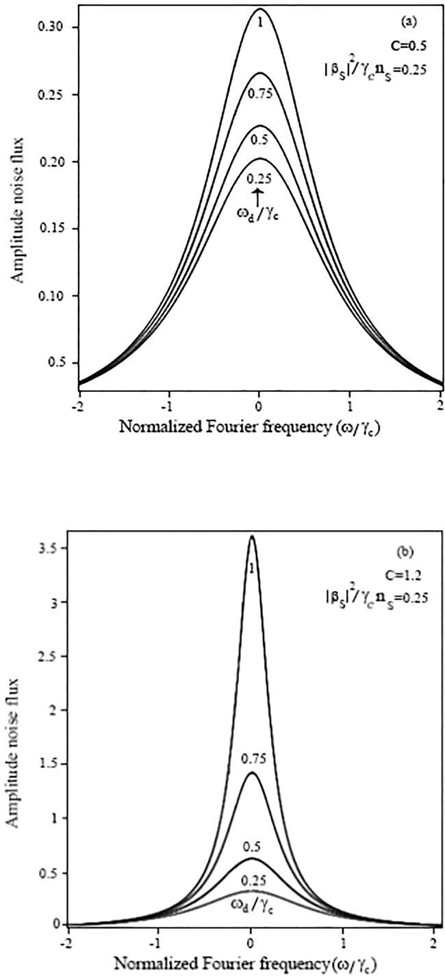
Figure 1. The Lorentzian profiles of amplitude noise flux are shown for a symmetrical cavity ${\gamma }_{1}={\gamma }_{2}={\gamma }_{C}$, different normalized frequency detuning ${\omega }_{d}/{\gamma }_{C}$, as indicated in the figures, for a typical normalized input signal flux ${\left|{\beta }_{S}\right|}^{2}/{\gamma }_{C}{n}_{s}=0.25$, and for two different normalized pumping rates (a) $C=0.5$ corresponding to the below-threshold state and (b) $C=1.2$ corresponding to the above-threshold state (injection-locked region). |
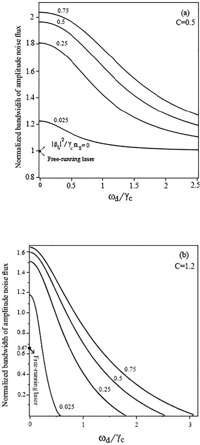
Figure 2. The normalized bandwidth ${({\rm{\Delta }}\omega )}_{{\rm{AM}}}^{{\rm{LA}}}/{\gamma }_{C}$ against the normalized frequency detuning ${\omega }_{d}/{\gamma }_{C}$ is plotted for various values of normalized input signal flux ${\left|{\beta }_{S}\right|}^{2}/{\gamma }_{C}{n}_{s}\,=$ 0, 0.025, 0.25, 0.5, and 0.75, as well as for the normalized pumping rates (a) $C=0.5$ and (b) $C=1.2$. It is evident that increasing the normalized frequency detuning ${\omega }_{d}/{\gamma }_{C}$ shortens the noise bandwidth of the laser amplifier, which is consistent with the findings in figure 1. The noise bandwidths of free-running laser (${\left|{\beta }_{S}\right|}^{2}/{\gamma }_{C}{n}_{s}$ = 0 and ${\omega }_{d}/{\gamma }_{C}$ = 0) are also represented on the vertical axis as single points, labeled 1 and 0.67, respectively. |
The impact of amplitude and frequency detuning of the input signal is shown in figure 2, where the normalized bandwidth ${({\rm{\Delta }}\omega )}_{{\rm{AM}}}^{{\rm{LA}}}/{\gamma }_{C}$ is plotted against the normalized frequency detuning ${\omega }_{d}/{\gamma }_{C}$ for various values of normalized input signal flux ${\left|{\beta }_{S}\right|}^{2}/{\gamma }_{C}{n}_{s}=$ 0, 0.025, 0.25, 0.5, and 0.75, as well as for the normalized pumping rates (a) $C=0.5$ and (b) $C=1.2$. By comparing figures 1 and 2, it is clear that the bandwidth of amplitude noise flux decreases as the normalized frequency detuning ${\omega }_{d}/{\gamma }_{C}$ increases, both in the below-threshold state and in the injection-locked regime of the laser amplifier. The specific values of 1 and 0.67, depicted in figures 2(a) and (b) are associated with the amplitude noise bandwidths of a free-running class-A laser (${\left|{\beta }_{S}\right|}^{2}/{\gamma }_{C}{n}_{s}=$ 0 and ${\omega }_{d}/{\gamma }_{C}$ = 0) in the below ($C=0.5$) and above ($C=1.2$) threshold states. These values will be calculated using the equations (30 ) and (33 ) in the next section.
Finally, the variations of amplitude noise flux ${N}_{{\rm{AM}}}^{{\rm{LA}}}(\omega )$ versus normalized Fourier frequency $\omega /{\gamma }_{C}$, as well as normalized bandwidth ${({\rm{\Delta }}\omega )}_{{\rm{AM}}}^{{\rm{LA}}}/{\gamma }_{C}$ against normalized frequency detuning ${\omega }_{d}/{\gamma }_{C}$, are respectively plotted in figures 3(a) and (b) at the critical (threshold) pumping rate $C=1$ under the same input signal parameters displayed in figures 1 and 2. A simple comparison of figures (1)–(3) indicates that the amplitude noise profiles and noise bandwidths of a laser amplifier exhibit similar behavior in the below-threshold $C\lt 1$, threshold $C=1$, and above-threshold $C\gt 1$ states. In other words, the behaviors of the below-threshold state, the threshold state, and the injection-locked regime of a laser amplifier resemble the above-threshold state of a free-running laser due to a single-component cavity electric field that oscillates at the input signal rather than cavity resonance frequency [2, 11]. In contrast, the amplitude noise profile and noise bandwidth of a free-running laser exhibit fundamentally different behavior at the critical threshold $C=1$. At this point, the noise bandwidth tends toward zero, ignoring both the input signal’s amplitude (${\beta }_{S}=0$) and frequency detuning (${\omega }_{d}=0$). This behavior will be discussed further in the next section.
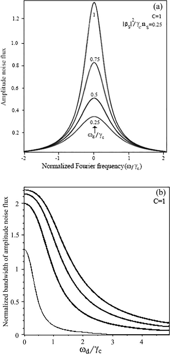
Figure 3. The variations of amplitude noise flux ${N}_{{\rm{AM}}}^{{\rm{LA}}}(\omega )$ versus normalized Fourier frequency $\omega /{\gamma }_{C}$, and normalized bandwidth ${({\rm{\Delta }}\omega )}_{{\rm{AM}}}^{{\rm{LA}}}/{\gamma }_{C}$ against normalized frequency detuning ${\omega }_{d}/{\gamma }_{C}$, are respectively plotted in parts (a) and (b) at the critical (threshold) pumping rate $C=1$ under the same input signal parameters shown in figures 1 and 2. The results indicate that the noise characteristics of a laser amplifier remain consistent across the below-threshold $C\lt 1$, threshold $C=1$, and above-threshold $C\gt 1$ states. |
Similarly, the noise fluxes of phase and spontaneous emission are derived by substituting their respective fluctuating variables $\delta {\varphi }_{S}(\omega )$ and $\delta {D}_{S}(\omega )$ from equations (14 ) and (15 ) into the correlation function relation given in equation (17 ) as20 ) does not display a specific profile, while the spontaneous emission noise flux (21) shows a Lorentzian profile with the same normalized bandwidth of 2B as the amplitude noise flux given by equation (19 ).
$\begin{eqnarray}\begin{array}{l}{N}_{{\rm{PH}}}^{{\rm{LA}}}(\omega )=2{\gamma }_{C}{\left|{\alpha }_{S}\right|}^{2}{\left|{h}_{{\rm{PH}}}^{{\rm{LA}}}\left(\omega \right)\,\right|}^{2}\\ \,=\,\displaystyle \frac{{\gamma }_{C}^{2}{B}^{2}+{\left(\omega +{\omega }_{d}\right)}^{2}}{{\omega }^{2}}{N}_{{\rm{AM}}}^{{\rm{LA}}}(\omega ),\end{array}\end{eqnarray}$
and $\begin{eqnarray}\begin{array}{l}{N}_{{\rm{SP}}}^{{\rm{LA}}}(\omega )=\displaystyle \frac{{\left|{h}_{{\rm{SP}}}^{{\rm{LA}}}(\omega )\right|}^{2}}{2{\gamma }_{C}{\left|{\alpha }_{S}\right|}^{2}}\\ \,=\,\displaystyle \frac{4\,{C}^{2}}{{\left(1+{\left|{\alpha }_{S}\right|}^{2}/{n}_{S}\right)}^{\,4}}{N}_{{\rm{AM}}}^{{\rm{LA}}}(\omega ).\end{array}\end{eqnarray}$
The phase noise flux (The role of laser pumping is to provide the necessary energy for amplifying an input signal according to the following energy conservation relation [8]22 ) can be rearranged to form a conservation relation for the fluctuating variables $\delta {\alpha }_{S}(t)$, $\delta {D}_{S}(t)$, and $\delta {D}_{P}(t)$ after substituting the trial solutions (5 ) and (6 ) as23 ) simplifies to that of a free-running laser after ignoring the input signal amplitude ${\beta }_{S}$ in agreement with equation (39) of [15].
$\begin{eqnarray}\begin{array}{l}2{\gamma }_{C}{\left|\alpha (t)\right|}^{2}-{\gamma }_{2}^{1/2}\left[{\alpha }^{\ast }(t){\beta }_{{\rm{in}}}+\alpha (t){\beta }_{{\rm{in}}}^{\ast }\right]\\ \,+\,{\gamma }_{| | }D(t)={\gamma }_{| | }D^{\prime} {}_{P}(t),\end{array}\end{eqnarray}$
where ${\gamma }_{| | }{D^{\prime} }_{P}(t)$ represents the total rate of pumping energy, which includes both the static mean value ${\gamma }_{| | }{D}_{P}$ and the fluctuating value ${\gamma }_{| | }\,\delta {D}_{P}(t)$. The energy conservation ( $\begin{eqnarray}\begin{array}{r}\begin{array}{c}4{\gamma }_{C}\left|{\alpha }_{S}\right|\delta {\alpha }_{S}(t)-\,2{\gamma }_{2}^{1/2}{\beta }_{S}\delta {\alpha }_{S}(t)\\ \,+\,{\gamma }_{||}\delta {D}_{S}(t)={\gamma }_{||}\delta {D}_{P}(t).\end{array}\end{array}\end{eqnarray}$
Here, $\delta {D}_{P}(t)$ acts as a fluctuating source for the other two variables $\delta {\alpha }_{S}(t)$ and $\delta {D}_{S}(t)$. The fluctuation conservation relation (3.1. The noise flux conservation
If one takes the Fourier transform of (23 ) and multiplies it by its complex conjugate, a flux conservation relation is derived for the noise fluxes of amplitude ${N}_{{\rm{AM}}}^{{\rm{LA}}}(\omega )$, spontaneous emission ${N}_{{\rm{SP}}}^{{\rm{LA}}}(\omega )$, and pumping ${N}_{{\rm{Pump}}}^{{\rm{LA}}}(\omega )$ using the correlation function (3 ) as23 ) as18 ), (21 ), and (26 ) respectively, satisfy the energy conservation relation (24 ).
$\begin{eqnarray}\begin{array}{l}4\,S\left({\beta }_{S},{\omega }_{d},C\right)\,{N}_{{\rm{AM}}}^{{\rm{LA}}}(\omega )+\,{N}_{{\rm{SP}}}^{{\rm{LA}}}(\omega )={N}_{{\rm{Pump}}}^{{\rm{LA}}}(\omega ),\end{array}\end{eqnarray}$
where $\begin{eqnarray}\begin{array}{c}S\left({\beta }_{S},{\omega }_{d},C\right)=\,1-\displaystyle \frac{{\beta }_{S}/\sqrt{{\gamma }_{C}{n}_{S}}}{\left|{\alpha }_{S}\right|/\sqrt{{n}_{S}}}\\ +\,\displaystyle \frac{{\beta }_{S}^{2}/{\gamma }_{C}{n}_{S}}{4\,{\left|{\alpha }_{S}\right|}^{2}/{n}_{S}}-\left(2-\displaystyle \frac{{\beta }_{S}/\sqrt{{\gamma }_{C}{n}_{S}}}{\left|{\alpha }_{S}\right|/\sqrt{{n}_{S}}}\right)\,\displaystyle \frac{{D}_{S}/{D}_{0}}{1+{\left|{\alpha }_{S}\right|}^{2}/{n}_{S}}.\end{array}\end{eqnarray}$
The normalized pumping noise flux ${N}_{{\rm{Pump}}}^{{\rm{LA}}}(\omega )$ is obtained differently by taking the Fourier transform of the fluctuation conservation relation ( $\begin{eqnarray}\begin{array}{l}{N}_{{\rm{Pump}}}^{{\rm{LA}}}(\omega )=\displaystyle \frac{\langle \left[{\gamma }_{| | }\delta {D}_{P}^{\ast }(\omega )\right]\,\left[{\gamma }_{| | }\delta {D}_{P}(\omega )\right]\rangle }{2{\gamma }_{C}{\left|{\alpha }_{S}\right|}^{2}}\\ \,=\,\left(2-\displaystyle \frac{{\beta }_{S}/\sqrt{{\gamma }_{C}{n}_{S}}}{\left|{\alpha }_{S}\right|/\sqrt{{n}_{S}}}-2\displaystyle \frac{{D}_{S}/{D}_{0}}{1+{\left|{\alpha }_{S}\right|}^{2}/{n}_{S}}\right)\,{N}_{{\rm{AM}}}^{{\rm{LA}}}(\omega ).\end{array}\end{eqnarray}$
It is straightforward to verify that the noise fluxes of amplitude, spontaneous emission, and pumping, as defined by equations (4. The noise fluxes of free-running class-A laser
The noise fluxes of a free-running laser can be directly extracted from those of the laser amplifier by ignoring the input signal’s amplitude ${\beta }_{S}$ and frequency detuning ${\omega }_{d}$ (${\omega }_{S}={\omega }_{L}$). Let us first consider the simpler case of the below-threshold state $(C\lt 1)$ so that in the absence of the cavity electric field ${\alpha }_{S}=0$, the atomic population inversion is reduced to ${D}_{S}=C{D}_{0}$ according to equation (8 ). The noise fluxes of amplitude (18 ), spontaneous emission (21 ), and pumping (26 ) have been simplified to
$\begin{eqnarray}{N}_{{\rm{AM}}}^{{\rm{BFL}}}(\omega )=\displaystyle \frac{{\gamma }_{C}^{2}}{2\pi \,\left[{\omega }^{2}+{\gamma }_{C}^{2}{(1-C)}^{2}\right]},\end{eqnarray}$
$\begin{eqnarray}{N}_{{\rm{SP}}}^{{\rm{BFL}}}(\omega )=4{C}^{2}{N}_{{\rm{AM}}}^{{\rm{BFL}}}(\omega ),\end{eqnarray}$
and $\begin{eqnarray}{N}_{{\rm{Pump}}}^{{\rm{BFL}}}(\omega )=4{(1-C)}^{2}{N}_{{\rm{AM}}}^{{\rm{BFL}}}(\omega ).\end{eqnarray}$
Here, the superscript BFL denotes the below-threshold free-running laser. It is noteworthy that we were unable to calculate the noise fluxes ${N}_{{\rm{SP}}}^{{\rm{BFL}}}(\omega )$ and ${N}_{{\rm{Pump}}}^{{\rm{LA}}}(\omega )$ in our previous noise analysis because there was no input signal (the free-running case), and the fluctuating variable $\delta D(t)$ turned out to be zero according to equation (10) of [15].Although the amplitude noise flux of BFL (27 ) has a coefficient difference of 4 in the numerator compared to its corresponding quantity (19) of [15], they share the same bandwidth as19 ) after applying the relevant conditions ${\alpha }_{S}={\beta }_{S}=0$ and ${D}_{S}=C{D}_{0}$. The bandwidth (30 ) was also derived by Loudon and his collaborators (LHSV), who ignored the cavity Langevin force ${{\rm{\Gamma }}}_{\alpha }=0$ and considered only the other two Langevin forces of the atomic population inversion ${{\rm{\Gamma }}}_{D}$ and atomic dipole moment ${{\rm{\Gamma }}}_{d}$ (see (4.27) and (4.28) of [13]). However, the noise flux conservation of the laser amplifier (24 ) is reduced to27 )-(29 ) into equation (31 ).
$\begin{eqnarray}{({\rm{\Delta }}\omega )}_{{\rm{AM}}}^{{\rm{BFL}}}=2{\gamma }_{C}(1-C),\end{eqnarray}$
which is apparent from the present laser amplifier bandwidth ( $\begin{eqnarray}4\,(1-2C){N}_{{\rm{AM}}}^{{\rm{BFL}}}(\omega )+\,{N}_{{\rm{SP}}}^{{\rm{BFL}}}(\omega )={N}_{{\rm{Pump}}}^{{\rm{BFL}}}(\omega ),\end{eqnarray}$
where this can be analytically verified by substituting the BFL noise fluxes (Finally, in the absence of a laser pumping rate $C=0$, there is no input pumping noise flux ${N}_{{\rm{Pump}}}^{{\rm{BFL}}}(\omega )=0$ to be distributed between the output spontaneous emission ${N}_{{\rm{SP}}}^{{\rm{BFL}}}(\omega )=0$ and amplitude ${N}_{{\rm{AM}}}^{{\rm{BFL}}}(\omega )=0$ noise fluxes. Therefore, the amplitude noise flux (27 ) is simplified to a Lorentzian profile in the form30 ) at the zero pumping rate $C=0$. This profile is in complete agreement with the Lorentzian spectrum of the empty cavity noise (cavity noise) derived by Scully and Zubairy in (9.3.12) of [34] and (20) of [15].
$\begin{eqnarray}{N}_{{\rm{AM}}}^{{\rm{BFL}}}(\omega )=\displaystyle \frac{{\gamma }_{C}^{2}}{2\pi \,\left({\omega }^{2}+{\gamma }_{C}^{2}\right)},\end{eqnarray}$
with a bandwidth equal to $2{\gamma }_{C}$ in accordance with equation (On the other hand, the above-threshold free-running laser (AFL) is distinguished by the different conditions ${\left|{\alpha }_{S}\right|}^{2}={\left|{\alpha }_{L}\right|}^{2}={n}_{S}(C-1)$ and ${D}_{S}={D}_{0}$ [8, 13] so that the noise fluxes of amplitude (18 ), spontaneous emission (21 ), pumping (26 ) and their conservation relation (24 ) exactly reproduce the corresponding AFL noise fluxes (34 ), (35 ), (43 ), and their conservation relation (46) of [15], respectively. The bandwidth of amplitude noise flux (19 ) is also simplified to
$\begin{eqnarray}{\left({\rm{\Delta }}\omega \right)}_{{\rm{AM}}}^{{\rm{AFL}}}=4{\gamma }_{C}\displaystyle \frac{C-1}{C},\end{eqnarray}$
which is in complete agreement with the free-running relations (5.62) of LHSV [13] and (47) of [15].5. The DFOTC and the coherence time of class-A laser amplifiers
According to the quantum optics literature [29, 35], the DFOTC of light is defined as a normalized version of the first-order correlation function in the form5 ). The statics amplitude ${\alpha }_{S}$ has already been utilized to study the gain behavior of class-A and -B laser amplifiers by calculating the normalized mean number of cavity photons ${\left|{\alpha }_{S}\right|}^{2}/{n}_{S}$ from the cubic equation (7 ) [8, 13]. In contrast, the present objective is to study the noise characteristics and DFOTC of class-A laser amplifiers using the temporal fluctuating variable $\delta {\alpha }_{S}(t)$. In other words, it is necessary to establish a relationship between the amplitude noise flux ${N}_{{\rm{AM}}}^{{\rm{LA}}}(\omega )$ and the degree of first-order temporal coherence ${g}_{{\rm{LA}}}^{(1)}(\tau )$.
$\begin{eqnarray}\begin{array}{l}{g}^{(1)}(\tau )={g}^{(1)}(t^{\prime} -t)\\ \,=\,\displaystyle \frac{\left\langle {\alpha }^{\ast }(t)\,\alpha (t^{\prime} )\right\rangle }{\left\langle {\alpha }^{\ast }(t)\,\alpha (t)\right\rangle }=\displaystyle \frac{\left\langle {\alpha }^{\ast }(t)\,\alpha (t+\tau )\right\rangle }{\left\langle {\alpha }^{\ast }(t)\,\alpha (t)\right\rangle },\end{array}\end{eqnarray}$
where $\alpha (t)$ represents the electric field of an arbitrary optical source whose interference pattern is measured by an optical interferometer with a delay time $\tau =t^{\prime} -t$ [28]. The cavity electric field $\alpha (t)$ is divided into the two components of statistics amplitude ${\alpha }_{S}$ and temporally fluctuating term $\delta {\alpha }_{S}(t)$ based on the trial solution (Let us consider the general definition of DFOTC (34 ) for a laser amplifier as34 ) by inspiring from the trial solution (5 ). The Fourier integral (35 ) can be calculated by substituting $\delta {\alpha }_{S}(\omega )$ from equation (13 ) and incorporating the correlation function of cavity Langevin force (3 ). The result is given by19 ). The physical significance of DFOTC ${g}_{{\rm{LA}}}^{(1)}(\tau )$ becomes apparent when it is related to the amplitude noise flux of the laser amplifier both within the laser cavity ${\left|{h}_{{\rm{AM}}}^{{\rm{LA}}}(\omega )\right|}^{2}$ and after it emerges from the cavity mirrors ${N}_{{\rm{AM}}}^{{\rm{LA}}}(\omega )$. This relationship can be analyzed using the following Fourier transform36 ) into equation (37 ), a Lorentzian profile is derived for the amplitude noise flux of the laser amplifier ${N}_{{\rm{AM}}}^{{\rm{LA}}}(\omega )$, which is consistent with equation (18 ). Meanwhile, the spontaneous emission and pumping noise fluxes are calculated by substituting ${N}_{{\rm{AM}}}^{{\rm{LA}}}(\omega )$ from equation (37 ) into equations (21 ) and (26 ), respectively. Thus, a key application of DFOTC ${g}_{{\rm{LA}}}^{(1)}(\tau )$ is to determine the various noise fluxes of a class-A laser amplifier.
$\begin{eqnarray}\begin{array}{l}{g}_{{\rm{LA}}}^{(1)}(\tau )={g}_{{\rm{LA}}}^{(1)}(t-t^{\prime} )=\,\left\langle \delta {\alpha }_{S}^{\ast }(t)\,\delta {\alpha }_{S}(t^{\prime} )\right\rangle \\ \,=\,\displaystyle \frac{1}{2\pi }\displaystyle \int {\rm{d}}\omega \,{{\rm{e}}}^{-{\rm{i}}\omega t}\displaystyle \int {\rm{d}}\omega ^{\prime} \,{{\rm{e}}}^{-{\rm{i}}\omega ^{\prime} t}\left\langle \delta {\alpha }_{S}^{\ast }(\omega )\,\delta {\alpha }_{S}(\omega ^{\prime} )\right\rangle ,\end{array}\end{eqnarray}$
where the neutral role of the statics quantity ${\alpha }_{S}$ has been canceled out from both the numerator and denominator of equation ( $\begin{eqnarray}{g}_{{\rm{LA}}}^{(1)}(\tau )=\,\displaystyle \frac{1}{4B}\displaystyle {\int }_{-\infty }^{\infty }{\rm{d}}\omega \,{{\rm{e}}}^{-{\rm{i}}\omega \tau }\displaystyle \frac{\gamma /\pi }{{\omega }^{2}+{\gamma }^{2}}=\displaystyle \frac{1}{4B}\,\exp \,(-\gamma \,\left|\tau \right|),\end{eqnarray}$
where the total damping rate of the laser amplifier $\gamma ={\gamma }_{C}B$ is represented as the product of the mean damping rate of cavity mirrors ${\gamma }_{C}$ and the dimensionless parameter B, which appears as the noise flux bandwidth of the laser amplifier in equation ( $\begin{eqnarray}\begin{array}{l}{N}_{{\rm{AM}}}^{{\rm{LA}}}(\omega )=2{\gamma }_{C}{\left|{h}_{{\rm{AM}}}^{{\rm{LA}}}(\omega )\right|}^{2}\\ \,=\,\displaystyle \frac{2{\gamma }_{C}}{\pi }\,\mathrm{Re}\,\left[\displaystyle {\int }_{0}^{\infty }{\rm{d}}\tau \,{{\rm{e}}}^{{\rm{i}}\omega \tau }{g}_{{\rm{LA}}}^{(1)}(\tau )\right].\end{array}\end{eqnarray}$
By substituting ${g}_{{\rm{LA}}}^{(1)}(\tau )$ from equation (Another important application of DFOTC relates to the coherence time ${\tau }_{c}$ of the light emitted from an optical source. Here, the coherence time ${\tau }_{c}^{LA}$ of a laser amplifier demonstrates a reverse relation with the damping rate of DFOTC (36 ) in the form19 ) and (38 ) reveals an uncertainty relation between the bandwidth of the amplitude noise flux ${\left({\rm{\Delta }}\omega \right)}_{{\rm{AM}}}^{{\rm{LA}}}$ and the coherence time ${\tau }_{c}^{{\rm{LA}}}$ of the laser amplifier in the form
$\begin{eqnarray}{\tau }_{c}^{{\rm{LA}}}=\displaystyle \frac{1}{\gamma }=\displaystyle \frac{1}{{\gamma }_{C}B}.\end{eqnarray}$
A straightforward comparison of equations ( $\begin{eqnarray}{\left({\rm{\Delta }}\omega \right)}_{{\rm{AM}}}^{{\rm{LA}}}\,{\tau }_{c}^{{\rm{LA}}}=2=cte.\end{eqnarray}$
6. The DFOTC and the coherence time of free-running class-A lasers
The DFOTC (36 ) is introduced here for the first time in the context of light passing through an amplifying medium, such as a laser amplifier. The below-threshold state of a free-running laser (BFL) is a special case that satisfies specific conditions ${\alpha }_{S}={\beta }_{S}=0$, ${\omega }_{d}=0$, and ${D}_{S}=C{D}_{0}$. Under these conditions, the relations (16 ), (36 ), (38 ), and (39 ) of class-A laser amplifiers are respectively simplified to41 ) into the general relation of amplitude noise flux (37 ). A Lorentzian profile is obtained for the amplitude noise flux of class-A lasers in complete agreement with equation (27 ). Furthermore, the bandwidth of the amplitude noise flux ${\left({\rm{\Delta }}\omega \right)}_{{\rm{AM}}}^{{\rm{BFL}}}\,=2{\gamma }_{C}(1-C)$, calculated by applying the coherence time ${\tau }_{{\rm{c}}}^{{\rm{BFL}}}$ from equation (42 ) into the uncertainty relation (43 ), exhibits consistency with the corresponding equations (4.28) of LHSV [13] and (21) of [15]. On the other hand, if one ignores the laser pumping rate ($C=0$), then equation (41 ) is simplified to ${g}_{{\rm{BFL}}}^{(1)}(\tau )=\,\tfrac{1}{4}\,\exp \,\left[-{\gamma }_{C}\,\left|\tau \right|\,\right]$. It reproduces the same Lorentzian noise profile of an empty cavity (32 ) by implementing equation (37 ). The coherence time (42 ) and bandwidth (43 ) satisfy the uncertainty relation ${\left({\rm{\Delta }}\omega \right)}_{{\rm{AM}}}^{{\rm{BFL}}}\,{\tau }_{{\rm{c}}}^{{\rm{BFL}}}=2$ in the absence of laser pumping ($C=0$).
$\begin{eqnarray}{B}_{{\rm{BFL}}}=1-C,\end{eqnarray}$
$\begin{eqnarray}{g}_{{\rm{BFL}}}^{(1)}(\tau )=\,\displaystyle \frac{1}{4(1-C)}\,\exp \,\left[-{\gamma }_{C}(1-C)\,\left|\tau \right|\,\right],\end{eqnarray}$
$\begin{eqnarray}{\tau }_{{\rm{c}}}^{{\rm{BFL}}}=\displaystyle \frac{1}{{\gamma }_{C}(1-C)},\end{eqnarray}$
and $\begin{eqnarray}{\left({\rm{\Delta }}\omega \right)}_{{\rm{AM}}}^{{\rm{BFL}}}\,=\displaystyle \frac{2}{{\tau }_{{\rm{c}}}^{{\rm{BFL}}}}=2{\gamma }_{C}(1-C).\end{eqnarray}$
The confirmation process of ${g}_{{\rm{BFL}}}^{(1)}(\tau )$ is straightforward by substituting equation (Another important case involves the above-threshold state of a free-running laser (AFL), for which the relations (16 ), (36 ), (38 ), and (39 ) have been respectively simplified to43 ) and (47 ), along with their corresponding coherence times (42 ) and (46 ) as a function of the normalized pumping rate $C$ in both the below-threshold state ($C\lt 1$) and the above-threshold state ($C\gt 1$). The uncertainty relation is evident throughout both regions, including at the critical border associated with the threshold state ($C=1$) so that the noise bandwidth approaches zero to counterbalance the divergent behavior of the coherence time.
$\begin{eqnarray}{B}_{{\rm{AFL}}}=\displaystyle \frac{2(C-1)}{C},\end{eqnarray}$
$\begin{eqnarray}{g}_{{\rm{AFL}}}^{(1)}(\tau )=\,\displaystyle \frac{C}{8\,(C-1)}\,\exp \,\left[-\displaystyle \frac{2{\gamma }_{C}(C-1)}{C}\,\left|\tau \right|\right],\end{eqnarray}$
$\begin{eqnarray}{\tau }_{{\rm{c}}}^{{\rm{AFL}}}=\displaystyle \frac{C}{2{\gamma }_{C}(C-1)},\end{eqnarray}$
and $\begin{eqnarray}{\left({\rm{\Delta }}\omega \right)}_{{\rm{AM}}}^{{\rm{AFL}}}=\displaystyle \frac{2}{{\tau }_{c}^{{\rm{A}}{\rm{F}}{\rm{L}}}}=\displaystyle \frac{4{\gamma }_{C}(C-1)}{C},\end{eqnarray}$
where the corresponding conditions ${\left|{\alpha }_{S}\right|}^{2}={\left|{\alpha }_{L}\right|}^{2}\,={n}_{S}(C-1)$ and ${D}_{S}={D}_{0}$ are used. Figure 4 shows the simultaneous variations of the normalized bandwidths of amplitude noise fluxes (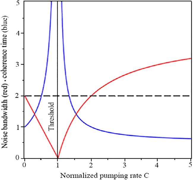
Figure 4. The simultaneous variations of noise bandwidth (the red curve) and coherence time (the blue curve) versus the normalized pumping rate C are plotted for the free-running laser in below and above-threshold states. The uncertainty principle, represented by the dashed line, is evident across all regions, including at the threshold state where the noise bandwidth approaches zero to balance the divergent behavior of coherence time. |
Finally, it is possible to reproduce the above-threshold amplitude noise flux of class-A lasers ${N}_{{\rm{AM}}}^{{\rm{LA}}}(\omega )$, as specified by equation (18 ), by applying ${g}_{{\rm{AFL}}}^{(1)}(\tau )$ from equation (45 ) to the amplitude noise flux relation (37 ), which is consistent with equation (34) of [15]. Similarly, the bandwidth of amplitude noise flux ${\left({\rm{\Delta }}\omega \right)}_{{\rm{AM}}}^{{\rm{AFL}}}=\tfrac{4{\gamma }_{C}(C-1)}{C}$ is derived by substituting the coherence time from equation (46 ) into the uncertainty relation (47 ). This fully agrees with the corresponding relations (5.62) of LHSV [13] and (47) of [15].
7. Conclusion
The impact of the cavity Langevin force as a source of fluctuations in the cavity electric field and atomic population inversion is discussed for a single-mode class-A laser amplifier in both below-threshold and above-threshold (injection-locked) states. These fluctuations are significant because the phase and amplitude noise fluxes arise from the correlation function of cavity electric field fluctuations, while the spontaneous emission noise flux stems from fluctuations in atomic population inversion. Although the phase noise flux (20 ) does not display a specific profile, both the amplitude noise flux (18 ) and the spontaneous emission noise flux (21 ) demonstrate Lorentzian profiles. These profiles have different peak values but share the same bandwidth (19 ), which is consistent with the noise profiles of a free-running laser as described by equation (47) of [15]. The primary source of amplitude and spontaneous emission noise fluxes is the input pumping noise flux, which are connected to each other by the flux conservation relation (24 ). It has been confirmed that the common bandwidth of input and output noise fluxes can be adjusted by varying the parameters of the input signal, such as amplitude and frequency detuning, along with the laser parameters, including the laser pumping rate and the mean damping rate of cavity mirrors.
The beneficial aspects of noise are explored here by linking the optical properties of a laser amplifier to the noise fluxes generated by the cavity Langevin force. For example, the DFOTC is defined as the correlation function of fluctuations in the cavity electric field according to equation (35 ). The damping rate of DFOTC is inversely related to the coherence time of the light emitted from the laser amplifier through equation (38 ). The Fourier transform of DFOTC yields the amplitude noise flux according to equation (37 ). Furthermore, the coherence time and bandwidth of the amplitude noise flux are connected by the uncertainty relation (39 ). It is observed that by increasing the frequency detuning or reducing the intensity of the input signal, the bandwidth of the amplitude noise flux decreases, as illustrated in figures (1)–(3). Finally, the relationship between the optical properties and noise fluxes of a class-A free-running laser is directly derived from those of a class-A laser amplifier by neglecting the amplitude (${\beta }_{S}=0$) and frequency detuning (${\omega }_{d}=0$) of the input signal.
Disclosures
The authors declare no conflicts of interest.