


1. Introduction
The quantum vacuum can be excited by some external stimulus like strong macroscopic electromagnetic fields (called vacuum polarization) [1]. Even at relatively low energies (relative to the Schwinger field strength ${E}_{{cr}}\,={m}_{e}^{2}{c}^{3}/e\hslash \simeq 1.32\times 1{0}^{18}\,{\rm{V}}\,{{\rm{m}}}^{-1}$), electron–positron pairs can be transiently created and annihilated (virtual particles), thereby interacting with the external fields [1, 2]. The measurement of the vacuum polarization effects has been underway since 1990s, such as Polarizzazione del Vuoto con LAser (PVLAS) and Biréfringence Magnétique du Vide (BMV) [3–6]. Recently, the development of high-power lasers, facilitated by the chirped pulse amplification technique, has reignited the interest in measuring such processes at ultrahigh laser intensities. Even though the current laser intensity has been able to reach the order of 1023 W cm−2 [7], the vacuum polarization signal in the experiment is still so weak that we have to resort to sophisticated instruments [8].
Among the various schemes that have been proposed or started to be implemented, the most eye-catching one should be the experiment driven by the vacuum birefringence effect [9]. This type of scheme is very promising because x-ray polarization detectors have already showcased outstanding accuracy, and it capitalizes on the fact that shorter wavelengths exhibit higher polarization flip rate [10–15]. There are other schemes such as combining the phase velocity change with detectors [16], combining the double slit interference [17, 18] or high-order harmonic effect with the single photon detector [19]. Despite the existence of several promising schemes, the pursuit of higher detection accuracy can help unveil previously unknown physical phenomena, such as the detection of axions [20]. Furthermore, it might extend theoretical verification to a broader parameter regime, especially given the current scarcity of potential schemes in the optical frequency range. Therefore, there is a strong motivation to explore new approaches to further enhance the measurement accuracy. However, the challenge lies in how to connect signals of vacuum polarization with the inherent accuracy of measuring instruments. In addition, finding a new detectable signal is essentially valuable. Compared to ongoing polarization signal detection schemes, it can provide a cross validation of quantum electrodynamics (QED) theory and give new dimensional information to explore polarization-blind particle models.
We find that frequency or spectrum information is an underestimated potential signal, despite some previous work discussing it [19, 21]. To make use of this signal in the experiment, we propose to employ the optical frequency comb (OFC). The OFC was developed nearly two decades ago to support the world’s most precise atomic clocks, which stands at forefront of the measurement precision [22]. The key features of the OFC are the ultrahigh frequency and time resolution. Recent progresses of a monolithic OFC can provide ultralow phase noise and an unprecedented frequency stability of 1 part in 1019 at a 1 s gate time [23]. Consequently, one significant application of the OFC lies in high-precision frequency measurement [24, 25]. Therefore, fully leveraging the characteristics of the OFC for frequency signal measurement holds significant promise for detect the quantum vacuum. However, to the best of our knowledge, research in this area remains unexplored.
In this paper, we propose a novel scheme to encode vacuum polarization signals into OFC to facilitate the experimental detection, where a tightly focused pump laser interacts with an OFC in its resonant cavity, see figure 1 for a more detailed description. We adapted the average variational approach [26, 27], where the OFC pulse can be treated as quasi-classical particles, and the nonlinearly responding vacuum acts as an effective potential for these particles. Our investigation reveals that by appropriately adjusting parameters of the pump laser such as the pulse duration, the focal spot size, and the time delay between pulse collisions, an obvious frequency shift of the OFC pulse can be obtained. This can be ascribed to the symmetry breaking by the tightly focused pump laser. In addition, we found that the presence of frequency upshift is always accompanied by the change in wave envelope. These vacuum polarization effects are eventually encoded into the properties of the OFC which are correlated to the parameters of ultrafast pump lasers. On the forthcoming laser systems, the measured signal of vacuum polarization surpasses the lowest resolution of OFC, which provides a new possibility for detecting vacuum polarization in the laboratory. The main results were verified and demonstrated through multi-dimensional particle-in-cell (PIC) simulations based on the quasi-classical method [28–30].
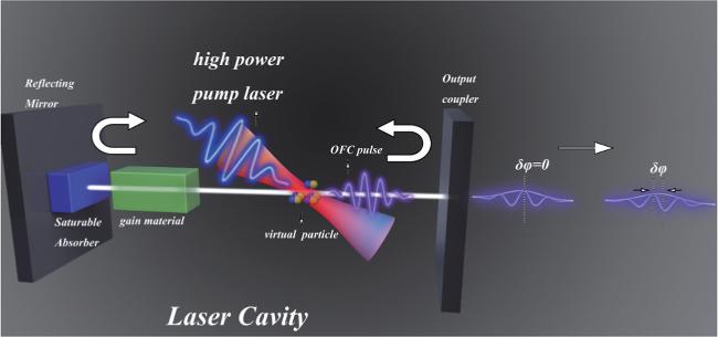
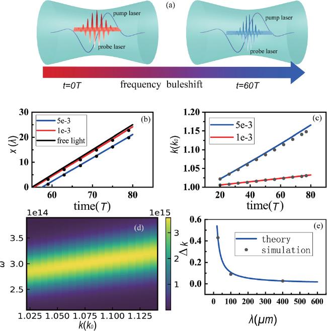
Figure 1. Schematic of the scheme for using OFC to probe the quantum vacuum. OFC is a phase-stabilized mode-locked laser [22]. In a typical passively mode-locked OFC resonant cavity, a saturable absorber causes a single pulse to gradually form in the cavity. Each pulse forms a smaller output pulse when passing through the output coupler, and then the main pulse is reflected back into the cavity and amplified by the gain medium. (Stabilized OFC also requires an external feedback loop to control the system that has not been drawn.) When the OFC pulse propagates to a certain position, a powerful tightly focused pump laser is injected from the outside to form a collision of two pulses. At this time, virtual particle-antiparticle pairs are generated and annihilated instantaneously, i.e. quantum fluctuations, which affect the properties of OFC pulse. |
2. Theoretical analysis
The OFC can be intuitively understood in the time domain as a series of nearly identical pulses emitted at a fixed repetition rate TR ≈ Lcavity/c, as illustrated in figure 1, where Lcavity is the length of the cavity and c is the light speed. It can be written as the convolution of a single pulse with a delta comb function:
$\begin{eqnarray}\begin{array}{rcl}E & = & \left(A(t)\exp ({\rm{i}}{\omega }_{c}t)\displaystyle \otimes \displaystyle \sum _{m=-\infty }^{\infty }\delta ({t}_{m})\right)\,\exp \,({\rm{i}}{\varphi }_{0}(t))\\ & = & \displaystyle \sum _{m=-\infty }^{\infty }A({t}_{m})\,\exp \,({\rm{i}}{\omega }_{c}({t}_{m})+{\rm{i}}{\varphi }_{0}(t)),\end{array}\end{eqnarray}$
where ⨂ represents the convolution, tm = t − mTR, ωc is the angular carrier frequency, A(t) is the pulse envelope, and φ0(t) is the absolute phase of the single pulse (the so-called carrier envelope offset (CEO) phase) which determines the difference between the optical phase of the carrier wave and the envelope position.The advancement of OFC technology relies on sophisticated stabilization techniques that ensure the pulse train sequence maintains highly stable parameters for each individual pulse. This stability is directly reflected in the spectral characteristics of the OFC. Specifically, OFC can be described in the frequency domain as a phase coherent optical Fourier modes: $E(t)={\sum }_{m=0}^{{m}_{f}}{A}_{m}\exp ({\rm{i}}{\omega }_{m}t)$ where each mode ωm/(2π) = fm = m · fR + fCEO is perfectly equidistant. We can see that all optical modes are phase coherent with one another, and fR = 1/TR relates to the interval between pulses, fCEO = (1/2π) · dφ(t)/dt relates to the CEO phase. These two key parameters of the OFC, fR and fCEO, can be controlled and measured with great accuracy using the nonlinear self-referencing method (detecting the heterodyne beat between two comb modes) [22, 25], which finally drove the OFC revolution around 2000. Recently, the linewidth of the spectral signal has reached mHz or even lower orders of magnitude [31]. This advancement naturally suggests leveraging the fact that even a slight shift in a specific mode (referred to as a ‘tooth’) of the OFC can be detected with a high signal-to-noise ratio (SNR).
Motivated by this, we aim to explore how to encode vacuum polarization effects into the OFC, particularly in terms of its spectral properties. Figure 1 and equation (1 ) illustrate that OFC can be viewed as a chain of pulses generated by a single main pulse traveling back and forth within the resonant cavity. Although the properties of the OFC are determined by the entire pulse train, we can first study the effect exerted by the vacuum polarization effect when the pump laser collides with a single main pulse. Hereafter, we refer to the single main OFC pulse as the probe pulse and the entire pulse train as the OFC. Equation (1 ) identifies several crucial parameters that warrant our attention, i.e. carrier ωc, envelope A(t) and the phase lag between them φ0(t). Hence, we first focus on analyzing the evolution of carrier frequency and wave envelope. Subsequently, we proceed to investigate the alterations in the properties of the OFC.
2.1. Ponderomotive effect induced by vacuum polarization
The starting point of the nonlinear quantum interaction in low-energy region, where the energy of photon is much smaller than the rest energy of electron, is the Heisenberg–Euler (H–E) Lagrangian [1, 2]. We assume that the strength of the involved electromagnetic field is much lower than the Schwinger limit Ecr, and the spatial scale of the field variation is much smaller than the Compton wavelength λc. Thus, we can use the so-called local constant field approximation and consider only the leading contribution to the H–E Lagrangian, as given in equation (2 ) for limits imposed by the experimental conditions
$\begin{eqnarray}{ \mathcal L }=-\frac{1}{4}\left({F}^{\mu \nu }{F}_{\mu \nu }\right)+\xi \left[{\left({F}^{\mu \nu }{F}_{\mu \nu }\right)}^{2}+\frac{7}{4}{\left(* {F}_{\mu \nu }{F}^{\mu \nu }\right)}^{2}\right]{\rm{,}}\end{eqnarray}$
where $\xi =2{\alpha }^{2}{\epsilon }_{0}^{2}{\hslash }^{3}/45{m}_{e}^{4}{c}^{5}\approx 1.3\times 1{0}^{-52}$ is the coupling parameter of vacuum polarization, *Fμν denotes the dual field strength tensor and α = e2/(4πϵ0ℏc) is fine-structure constant. We set c = ℏ = 1 next unless otherwise specified.To address the problems about quantum vacuum effect in the equation above, we can either solve for the E–L equation corresponding to the Lagrangian and apply the Green’s function method to the first order [10], or alternatively, use the ‘vacuum emission’ method [32]. In most cases, these methods are sufficient for analysis. They transform the problem into evaluating the Fourier integral of a complex field distribution and thus providing the far-field differential number of signal photons d3N/dk3. However, since the standard method for measuring OFC is self-referencing, we must consider the photon coherence or obtain a macroscopic description of the OFC. If the aforementioned method is used, additional integration of the scattered signal photons is required. Due to the complex form of the integral, obtaining an analytical solution is challenging. Therefore, to address this issue and focus on the key physics, here, we adopt the ‘average variational approach’ [26, 27].
For any Lagrangian describing the vector potential, ${ \mathcal L }=\iint { \mathcal L }({\partial }_{t}A,{\rm{\nabla }}A,A)\,{{\rm{d}}}^{3}x{\rm{d}}t$, A has a solution that involves modulation based on some characteristic form (with slowly varying parameters). In our case, the vector potential A corresponds the probe laser and is expected to be modulated by vacuum polarization on the basis of the incident periodic pulse, A = Φ(θ, x, t). Here, Φ is a periodic function of θ (with the period normalized to 2π). We define the following parameters for this wavetrain: the local wave vector and the local frequency k(x, t) = ∇ θ, ω(x, t) = − ∂tθ. The average variational approach allows us to directly study the evolution of these parameters by introducing the following average Lagrangian 3 ) including the approximations and derivations involved are included in the appendix and, our later analyses and PIC simulations will help justifying the simplification.
$\begin{eqnarray}\begin{array}{rcl}\bar{{ \mathcal L }} & = & -\frac{1}{4}{a}^{2}\left({k}^{2}-{\omega }^{2}+\frac{1}{2}{A}_{N}\left({k}^{2}+2k\omega +{\omega }^{2}\right)\right)\\ & & -\frac{1}{8}{A}_{N}\left({\left({\partial }_{x}a\right)}^{2}-2{\partial }_{t}a{\partial }_{x}a+{\left({\partial }_{t}a\right)}^{2}\right){\rm{,}}\end{array}\end{eqnarray}$
where the probe laser is assumed as ${\boldsymbol{E}}={{\boldsymbol{e}}}_{i}a({\boldsymbol{x}},t)\,\exp \,({\rm{i}}\theta (x,t))$ and the pump laser is ${{\boldsymbol{E}}}_{\,\rm{pump}\,}({\boldsymbol{x}},t)={{\boldsymbol{e}}}_{y}{E}_{0}({\boldsymbol{x}},t)\cdot \exp ({\rm{i}}{\rm{\Theta }}(x,t))$, ${A}_{N}=14\xi {E}_{0}^{2}({\boldsymbol{x}},t)/{\varepsilon }_{0}$ if ei is z direction, ${A}_{N}=8\xi {E}_{0}^{2}({\boldsymbol{x}},t)/{\varepsilon }_{0}$ if ei is y direction. E0(x, t) is the envelope of the pump laser. Note that here, for clarity and to illustrate the main physics, we consider the case of head-on collisions between the probe laser and the pump laser. A detailed explanation of equation (Then, using the variational principle for a and consistency relations, we can obtain the ray-equation that can represent the main characteristic dynamics of probe photon [26, 27]3 ) extracts the low-frequency effects of the rapidly oscillating pump field on the incident probe laser (see appendix), equation (4 ) describes the evolution process of position x and momentum (wave vector) k of the probe laser under the background pump field. This allows us to treat the probe pulse as a quasi-classical particle, with the nonlinearly responding vacuum acting as an effective potential for these particles. In this context, the evolution of the photon momentum depends on the gradient of the pump laser envelope, which is similar to the well-known expression for the ponderomotive force experienced by electrons in a laser field [33]. Following the terminology in the literature [34], we refer to this effect as the ponderomotive force for photons.
$\begin{eqnarray}\begin{array}{rcl}\dot{{\boldsymbol{x}}} & = & \left(1-{A}_{N}({\boldsymbol{x}},t)+\frac{{M}_{N}}{4a{k}^{2}}\right)\hat{{\boldsymbol{k}}}{\rm{,}}\\ \dot{{\boldsymbol{k}}} & = & -k{\rm{\nabla }}\left(1-{A}_{N}({\boldsymbol{x}},t)+\frac{{M}_{N}}{4a{k}^{2}}\right){\rm{,}}\end{array}\end{eqnarray}$
where MN = (∂x − ∂t)(AN∂ta − AN∂xa). While equation (As mentioned above, we also need to apply the variational principle to θ. This gives the evolution of the envelope and the relationship between the envelope and the carrier 4 ).
$\begin{eqnarray}\begin{array}{l}(2\omega +k{A}_{N}+\omega {A}_{N}){\partial }_{t}{a}^{2}\\ -(-2k+\omega {A}_{N}+k{A}_{N}){\partial }_{x}{a}^{2}\\ +{a}^{2}(\omega -k)({\partial }_{t}{A}_{N}-{\partial }_{x}{A}_{N})=0{\rm{.}}\end{array}\end{eqnarray}$
The solution to this equation can be written as the form $\begin{eqnarray}\begin{array}{rcl}{a}^{2}({\boldsymbol{x}},t) & = & {\hat{s}}_{-t}{a}_{0}^{2}({\boldsymbol{x}})\\ & & +{\displaystyle \int }_{0}^{t}{\hat{s}}_{{t}^{{\prime} }-t}(-{a}^{2}(\omega -k)({\partial }_{t}{A}_{N}-{\partial }_{x}{A}_{N})){\rm{d}}{t}^{{\prime} }{\rm{.}}\end{array}\end{eqnarray}$
The ${\hat{s}}_{-t}$ operator functions to rewind the variable x to its state at time t at a speed governed by $\frac{-(-2k+\omega {A}_{N}+k{A}_{N})}{(2\omega +k{A}_{N}+\omega {A}_{N})}\approx {v}_{g}$. This solution can be intuitively understood as treating each point on the probe laser as an independent particle, carrying definite intensity information. Each particle moves at a velocity of vg while changing its intensity at a rate of (−a2(ω − k)(∂tAN − ∂xAN)). Thus, vg represents the moving speed of the envelope, i.e. the group velocity. In fact, vg is exactly the speed of x in equation (2.2. Effect induced by ponderomotive force
In the following, we will focus on three primary effects induced by the ponderomotive force. The first corresponds to the change in the spectrum, especially the carrier. Equation (4 ) intuitively shows the main behavior that the frequency of photons increase at the rising edge and decrease at the falling edge of the pump envelope. This result can also be understood from the perspective of equation (6 ). Since each point on the probe laser carries intensity information with velocity vg, equation (4 ) indicates a non-zero ponderomotive force ($\dot{{\boldsymbol{k}}}\ne 0$) implying a spatial inhomogeneity of these velocities, leading to a change in the wave envelope. When the probe laser is located on the rising edge of the pump laser envelope, it will be compressed due to the slow motion of the front point and the fast motion of the back point. We know that the compression of the spatial spreading distribution corresponds to an increase in frequency and this also leads to a certain degree of broadening of the spectrum.
Secondly, the phase velocity of the carrier can be obtained from the dispersion relation equation (A.3 ),
$\begin{eqnarray}{v}_{p}\approx 1-{A}_{N}({\boldsymbol{x}},t)-\frac{{M}_{N}}{4a{k}^{2}}{\rm{.}}\end{eqnarray}$
Combined with the velocity of the envelope given by vg, we can obtain the change of CEO phase.The third is the change in the intensity of the probe laser. In experimental measurements, we tend to focus on the electric field information 4 ), and the evolution of ∂ta can be obtained by taking the time derivative of equation (5 ). Finally, by substituting these results into equation (8 ), we can obtain the evolution of the electric field amplitude 9 ) indicates that the probe laser intensity will gradually increase or decrease depending on ∂tvg.
$\begin{eqnarray}\begin{array}{rcl}E & = & -{\partial }_{t}A=-{\partial }_{t}(a\cos (\theta (x,t)))\\ & = & \sqrt{{({\partial }_{t}a)}^{2}+{a}^{2}\omega {(x,t)}^{2}}\cos (\theta (x,t)-{\theta }^{{\prime} }){\rm{.}}\end{array}\end{eqnarray}$
The evolution of ω(x, t) can be obtained from equation ( $\begin{eqnarray}{\partial }_{t}| E| +{v}_{g}{\partial }_{x}| E| =\frac{{\partial }_{t}{v}_{g}}{{v}_{g}}| E| {\rm{.}}\end{eqnarray}$
Its solution is $|E|\,=\,|{E}_{0}|\,\exp \,\left({\rm{i}}\frac{{{\rm{\partial }}}_{t}{v}_{g}}{{v}_{g}}\tau \right)$ in the light speed frame, with ξ = x − ∫vgdt, τ = t. The right-hand term of equation (To verify our theory and conduct further analysis of our proposed scheme, we carried out 2D PIC simulations. We have developed a vacuum polarization module and integrated it into the EPOCH code [28]. The appendix includes some more specific explanations of the simulation program and supplementary simulations that may be helpful for understanding.
We firstly preform two simulations by colliding a Gaussian probe laser with a pump field with and without oscillating component. The envelope intensity of the pump field increases linearly along the propagation direction of the probe pulse, as depicted in figure 2(a). The temporal evolution of the maximum wave vector, FWHM of spectrum, and highest strength of the probe laser during the collision is shown in figures 2(b), (c), and (d), respectively. It is worth noting that the maximum wave vector in figure 2(b) does not exhibit an oscillatory feature like the strength evolution in figure 2(d), but rather a low-frequency rising process. This can be understood from the uncertainty principle, which makes it impossible to define the wave vector for the precise physical location. Hence, the wave vector of the probe laser can only be analyzed within an appropriately wide window, leading to a spatial averaging effect. This is also one of the reasons why the averaged Lagrangian in equation (3 ) is valid here. In any case, the comparison of the simulated and theoretical results clearly shows that the average variational method and the ponderomotive force equation (4 ) can effectively describe the evolution of the probe laser.
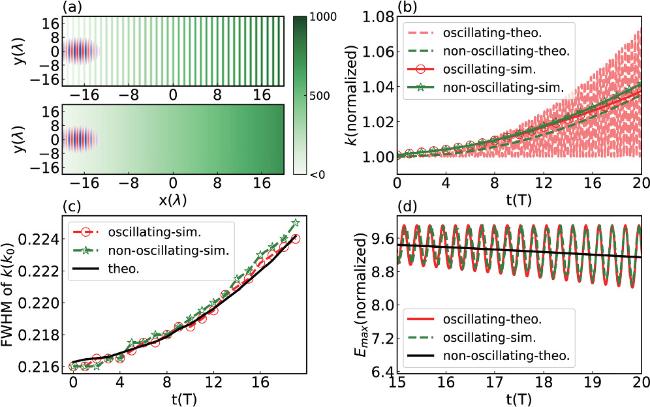
Figure 2. (a) Schematic of a probe laser with a Gaussian temporal profile passing through a pump field with an oscillating (upper panel) and non-oscillating (lower panel) increasing profile. The colormap represents the strength of the pump fields (normalized by mecω0/e). The slope of the oscillating field is $\sqrt{2}$ times larger than that of non-oscillating filed, which, according to the theoretical analysis, makes the probe laser to behave similarly in both cases. (b), (c), (d) temporal evolution of the carrier wave vector, FWHM of spectrum, and highest strength during the collision of the probe laser, respectively. |
3. Main results
3.1. Photon acceleration by tightly focused pump laser
As shown in figure 1, a tightly focused strong pump laser is injected into the OFC resonant cavity. For a single collision, consider a two-dimensional tightly focused Gaussian laser as an example
$\begin{eqnarray}\begin{array}{rcl}{E}_{\rm{pump}} & = & {E}_{\rm{pump0}}\sqrt{\frac{{w}_{0}}{w(x)}}\exp \left(-\frac{{y}^{2}}{{w}^{2}}+{\rm{i}}{\rm{\Phi }}\right),\\ {\rm{\Phi }} & = & kx+\frac{k{y}^{2}}{2x\left[1+{\left(\frac{{x}_{R}}{x}\right)}^{2}\right]}-\frac{1}{2}\arctan \left(\frac{x}{{x}_{R}}\right),\\ {E}_{\rm{pump0}} & = & {E}_{0}\exp \left(-\frac{{\left[t-{\tau }_{0}+\frac{x}{c}-\frac{{y}^{2}}{2{cR}(x)}\right]}^{2}}{{\rm{\Delta }}{\tau }^{2}}\right),\end{array}\end{eqnarray}$
where $w(x)={w}_{0}\sqrt{1+{((x-{x}_{0})/{x}_{R})}^{2}}$ is beam waist, ${x}_{R}=\pi {w}_{0}^{2}/\lambda $ is Rayleigh length, and $R(x)=x(1+{x}_{R}^{2}/{x}^{2})$ is radius of curvature. x0 represents focal spot position of pump laser, τ0 represents the time when pump pulse reaches x = 0.Using equations (4 ) and (10 ), taking only the first order into account, after some simplification, we have the final frequency shift 3 ) can be expressed in the form of canonical equations, thereby allowing the use of canonical transformations. By applying the canonical transformation $q=\bar{x}+ct,p=k$ to the effective potential field, we can demonstrate that when the pump resembles a one-dimensional plane wave $f({\rm{\Phi }})=a(-{k}_{-}(\bar{x}+ct))\cdot \exp (-{\rm{i}}{k}_{-}(\bar{x}+ct))$, the probe laser does not gain any energy from the collision. This suggests that when the pump laser has Gaussian profile with a large beam waist, it can be approximated as a one-dimensional wave, resulting in no final frequency shift for the probe laser. In our case, if x0 deviates a little from cτ0/2, the tight focusing effect (i.e. the denominator term) will break the symmetry. From the formula, it is appropriate to perform a Taylor expansion of the integral around x0 = cτ0/2 (using variable substitution ${z}^{{\prime} }=({(c\tau -{x}_{0})}^{2}/{x}_{R}^{2})$). This gives
$\begin{eqnarray}\begin{array}{c}{\rm{\Delta }}k(\xi ,\tau )\\ \,={\displaystyle \int }_{0}^{\tau }\frac{-56\xi {E}_{0}^{2}\exp \left(\frac{-2{(\xi +2c\tau -c{\tau }_{0})}^{2}}{{c}^{2}{\rm{\Delta }}{\tau }^{2}}\right)(\xi +2c\tau -c{\tau }_{0})}{{c}^{2}{\rm{\Delta }}{\tau }^{2}\sqrt{1+{\left(\frac{\xi +c\tau -{x}_{0}}{{x}_{R}}\right)}^{2}}}\\ \,+\frac{-\xi {E}_{0}^{2}\,\exp \,\left(\frac{-2{(\xi +2c\tau -c{\tau }_{0})}^{2}}{{c}^{2}{\rm{\Delta }}{\tau }^{2}}\right)(\xi +2c\tau -c{\tau }_{0})}{4{x}_{R}^{2}{\left(1+{\left(\frac{\xi +c\tau -{x}_{0}}{{x}_{R}}\right)}^{2}\right)}^{-3/2}}\,\,{\rm{d}}\tau .\end{array}\end{eqnarray}$
If ξ + 2cτ − cτ0 < 0, Δk increases in the time of dτ, and vice versa. Note that when x0 = cτ0/2 or xR → ∞, for ξ = 0, the integrand is an odd function, and the entire integral value is 0. This corresponds to that the probe laser passes through the pump laser completely symmetrically, and the acceleration and deceleration experienced by the probe laser cancel each other out. In fact, equation ( $\begin{eqnarray}\begin{array}{rcl}{\rm{\Delta }}k(\tau ) & = & 2{\int }_{0}^{\tau }\frac{28\xi {E}_{0}^{2}\exp \left(\frac{-8{x}_{R}^{2}{z}^{{\rm{{\prime} }}}}{{c}^{2}{\rm{\Delta }}{\tau }^{2}}\right)}{{c}^{2}{\rm{\Delta }}{\tau }^{2}}\\ & & \times \,\frac{{x}_{R}}{c}\sqrt{{z}^{{\rm{{\prime} }}}}{({z}^{{\rm{{\prime} }}}+1)}^{-\frac{3}{2}}{\rm{\Delta }}{x}_{0}{\rm{d}}{z}^{{\rm{{\prime} }}}.\end{array}\end{eqnarray}$
We performed PIC simulations to analyze the above process more carefully, as shown in figure 3(a). The size of the simulation box is (−10 ∼ 10λ) × (−15 ∼ 15λ), where 4000 × 600 cells are divided in the x and y directions, respectively. A Gaussian pump laser was incident from the right boundary into the box, with a peak intensity of 1.37 × 1024 W cm−2 (a = 1000), wavelength λ = 1 μm, pulse duration FWHM Δτ = 5T, and beam waist w0,pump = 1λ. The focal spot was positioned at x = 0. After a delay, a probe laser, also Gaussian, was incident from the left boundary with amplitude a = 10, wavelength λ = 1 μm, FWHM of pulse duration τ = 2T, and beam waist wprobe = 8λ. Its focal spot position was also set at x = 0. The nonlinear parameter ξ was set to 4.3 × 10−45 in this simulation (ξE2 ∼ 5e−3 see appendix for justification). When the pump laser is at the x = 0, the probe laser is at −5 μm. Thus, the pump laser passes through the center of the simulation box and subsequently collides with the probe laser.
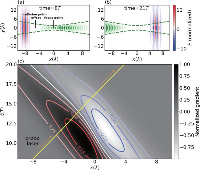
Figure 3. (a), (b) The intensity map of the pre- and post-collision of the probe laser and the pump laser. (c) The probe laser experiences a stronger positive gradient in the whole interaction process. The yellow line represent the trajectory of the probe laser and the background contour diagram shows the spatial distribution of the gradient of the pump laser envelope (here only the data on the central axis y = 0 are shown). |
Figure 3(b) displays the two-dimensional electric field distribution of the probe laser after the collision. We can intuitively see that because the pump laser has a narrow beam waist, the electric field near y = 0 changes after the interaction, i.e. a phase delay occurs due to the presence of a strong pump field that changes the refractive index. For the near-field evolution that occurs when two lasers interact, we expect the basic behavior of the probe laser to be similar to that shown in figure 2, in which the most important thing is the gradual change in the carrier frequency. To provide a more intuitive understanding of the physical processes involved, we present a plot that shows the trajectory of the probe laser (yellow line) and the gradient of the laser envelope amplitude (shown as a contour diagram) in the same figure figure 3(c). Between approximately 8T − 14T, the probe laser collides with the pump laser, experiencing a positive gradient that results in a frequency upshift (blank region). Its frequency reaches a peak of 1.035k0 at around 14T. As the probe laser is about to move away from the pump laser, it experiences a negative gradient, causing the wave-vector to gradually shift down (white region). However, due to the presence of the factor $\sqrt{{w}_{0}/w(x)}$ in tightly focused lasers, we observe that the yellow line experiences a larger gradient in the blank region than in the white region (see the value marked by contour line). It is this symmetry breaking that ultimately leads to photon acceleration. Figure 4(a) shows the spectrum evolution of the electric field on axis y = 0. We can see that the spectrum undergoes an overall right shift followed by a left shift, which corresponds to a rise and then a fall in the carrier frequency. At t = 21T, the probe laser has completely left the pump laser and gets a final frequency rise 1.01k0.
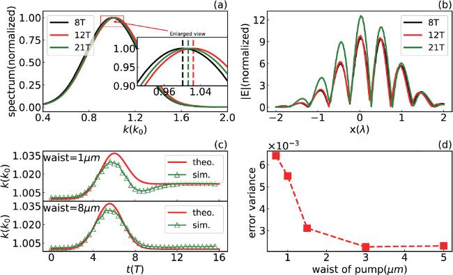
Figure 4. (a) The normalized spectrum of kx of the probe laser on the axis at 8T, 12T, 21T. (b) The electric field Ez of the probe laser as a function of position x on the axis at the initial and final states. (c) The time evolution of carrier kx on the axis for the cases w0,pump = 1 μm (upper) and wpump = 8 μm (lower). The theoretical lines are calculated from equations ( |
3.2. OFC signal influenced by vacuum polarization
As previously mentioned, the properties of OFC is that of a whole chain of pulses, so we now return to the analysis of the entire OFC. In the schematic shown in figure 1, a continuously injected pump laser can collide with OFC pulse multiple times. It may accumulate the vacuum polarization effect over a given measurement time, so we broaden the scope of pump lasers under consideration, ranging from ultra-intensity and ultra-fast lasers commonly used in other vacuum polarization experiments such as ELI-NP [35] (very high peak power 10 PW with 1 shot per minute) to a wider range of ultra-fast laser systems [36, 37] (relatively low peak power but the repetition rate can reach 100 MHz or more). In general, the pursuit of higher intensity can produce a strong measurement signal in a single collision, which is conducive to reduce the measurement time and mitigate the impact of other disturbance factors. However, the use of a high repetition rate laser allows for higher average power and provides us with more possibilities to modulate the OFC and vacuum polarization signals. So, there is a trade-off between the repetition rate and the peak intensity of the focused pump laser. To briefly illustrate the principle of possible OFC property changes, we leave aside the specific parameters for the moment and assume the OFC pulse in the resonator can collide with the pump laser at the same position during each round-trip. As stated above, we will focus on changes in OFC frequency information as potential measurable signals.
The modifications in the properties of the OFC can originate from two sources: the immediate alterations in properties following the collision of pulses (called direct change), and the subsequent effects that occur during the transmission within the resonant cavity (called indirect change). Regardless of the type of pump source, these modifications can be included in the expression of the pulse train represented below.
$\begin{eqnarray}\begin{array}{rcl}E(t) & = & \displaystyle \sum _{m=-\infty }^{\infty }\,A({t}_{m}^{{\rm{{\prime} }}})(1+m\delta A(t))\exp ({\rm{i}}{\omega }_{c}({t}_{m}^{{\rm{{\prime} }}}))\\ & & \times \,\exp \left({\rm{i}}{\varphi }_{0}(t)+{\rm{i}}\delta {\varphi }_{0}(t)\right)\times \exp ({\rm{i}}\,m\delta \omega ({t}_{m}^{{\rm{{\prime} }}})),\end{array}\end{eqnarray}$
where δA(t) is the amplitude change, δφ0(t) is the CEO phase change, ${t}_{m}^{{\prime} }=t-m{T}_{R}^{{\prime} },{T}_{R}^{{\prime} }={T}_{R}+\delta {T}_{R}$ is caused by the refraction index change (phase delay), $\exp ({\rm{i}}\,m\delta \omega ({t}_{m}^{{\prime} }))$ represents the carrier frequency shift after every collision.Let us consider separately how these changes constitute a possible OFC measurement signal. Firstly, we refer to the tips in [25] to calculate the frequency shift term $\exp ({\rm{i}}m\delta \omega ({t}_{m}))$ which is a pure direct change. Let ${ \mathcal F }$ denote the Fourier transform and ${ \mathcal F }\left\{A(t)\right\}=\tilde{A}(\omega )$, we have
$\begin{eqnarray}\begin{array}{l}{ \mathcal F }\left\{\displaystyle \sum _{m=-\infty }^{\infty }A({t}_{m})\exp ({\rm{i}}{\omega }_{c}({t}_{m}))\exp ({\rm{i}}\,m\delta \omega ({t}_{m}))\right\}\\ \quad \approx \displaystyle \sum _{m=-\infty }^{\infty }{\tilde{A}}_{c}\exp (-{\rm{i}}\omega m{T}_{R})\\ \quad +\displaystyle \sum _{m=-\infty }^{\infty }\frac{{\rm{i}}{\tilde{A}}_{c}^{{\prime} }}{{T}_{R}}\left\{({\rm{i}}\,m\delta \omega {T}_{R}+1)-1\right\}\exp (-{\rm{i}}\omega m{T}_{R})\\ \quad =\displaystyle \sum _{m=-\infty }^{\infty }{c}_{0}\delta (\omega -m{\omega }_{T})+{c}_{1}\delta (\omega -m{\omega }_{T}-\delta \omega ){\rm{.}}\end{array}\end{eqnarray}$
Here, ${\tilde{A}}_{c}=\tilde{A}(\omega -{\omega }_{c})$, we do a first-order Taylor expansion on $\tilde{A}(\omega -{\omega }_{c}-m{\omega }_{c})$ with respect to mωc and denote ${\tilde{A}}_{c}^{{\prime} }={\tilde{A}}^{{\prime} }(\omega -{\omega }_{c})$. ${c}_{0}=({\tilde{A}}_{c}-{\rm{i}}\frac{{\tilde{A}}_{c}^{{\prime} }}{{T}_{R}}),{c}_{1}={\rm{i}}{\tilde{A}}_{c}^{{\prime} }\frac{1}{{T}_{R}}$. We have used the relation ${\sum }_{m=-\infty }^{\infty }\exp (-{\rm{i}}\omega m{T}_{R})={\sum }_{m=-\infty }^{\infty }$δ(ω − mωT), ωT = 2π/TR. The above equation holds only for a very small δω, specially NδωTR < 1, where N is the actual number of pulses generated during the experiment measurement, and 1/(N · TR) is approximately equal to the theoretical linewidth of the OFC. Thus, the direct contribution of the frequency rise term to the OFC spectrum is to produce a small sideband with a frequency shift δω, whose normalized intensity power is (compared to the peak intensity of the carrier signal). $\begin{eqnarray}{\tilde{P}}_{\delta \omega }=10\mathrm{lg}({P}_{\delta \omega }/{P}_{\,\rm{carrier}\,})\approx 20\mathrm{lg}\left(\displaystyle \frac{{\rm{\Delta }}{\tau }_{\,\rm{probe}\,}}{{T}_{R}}\right){\rm{d}}B{\rm{,}}\end{eqnarray}$
where Δτprobe is the pulse duration of the probe laser.Secondly, analyzing the impact of ${T}_{R}^{{\prime} }={T}_{R}+\delta {T}_{R}$ on the OFC is simpler, as it directly changes ${f}_{R}^{{\prime} }=1/{T}_{R}^{{\prime} }$, causing each comb tooth to move δf = m · δfR = m · fR · (δTR/TR). The corresponding overall shift of the comb tooth frequency at the carrier frequency is approximately
$\begin{eqnarray}{\rm{\Delta }}\omega \approx {A}_{N}\times \frac{{\rm{\Delta }}{\tau }_{\rm{pump}}}{{T}_{R}}\times {\omega }_{c}.\end{eqnarray}$
Thirdly, we already know that the CEO phase is directly related to the fCEO of OFC. Our focus now is on analyzing the possible sources of δφ0(t). By definition, the CEO phase is the relative displacement between the carrier and envelope, usually caused by vg ≠ vp.4 ) and (7 ) demonstrate that vg is not equal to vp during the pulse collision, resulting in a direct change of the CEO phase.18 ), (19 ) indicate a constant shot-to-shot phase difference, and therefore we can assume a linearly evolving absolute phase ${\varphi }_{0}(t)=2\pi {f}_{{\rm{CEO}}}t=2\pi \frac{\,\mathrm{mod}\,({\rm{\Delta }}\varphi ,2\pi )}{{T}_{R}}t$. Accordingly, we can obtain the physical quantity fCEO that we wish to obtain.
$\begin{eqnarray}{\rm{\Delta }}\varphi =\omega {\int }_{0}^{L}\left(-\frac{1}{{v}_{g}}+\frac{1}{{v}_{p}}\right){\rm{d}}x.\end{eqnarray}$
Equations ( $\begin{eqnarray}{\rm{\Delta }}{\varphi }_{d}=-\omega {\int }_{c}\frac{{M}_{N}}{2a{k}^{2}}{\rm{d}}x,\end{eqnarray}$
where c represents the collision area. In addition, there is a more important source of indirect change for δφ0(t). In the absence of vacuum polarization, the main source of origin CEO phase φ0(t) is that the material inside the resonator is a dispersive medium whose vg ≠ vp. So it can be calculated by integrating along the beam path of one cavity round trip [24]. $\begin{eqnarray}{\varphi }_{0}={\int }_{0}^{L}\left(-\frac{\omega }{{v}_{g}}+\frac{\omega }{{v}_{p}}\right){\rm{d}}x={\int }_{0}^{L}\frac{{\omega }^{2}}{c}\frac{{\rm{d}}n(\omega ,x)}{{\rm{d}}\omega }{\rm{d}}x{\rm{.}}\end{eqnarray}$
We can see that φ0 depends on the carrier frequency. As the pump light induces a shift in the carrier frequency, it consequently affects the propagation of the OFC pulse within the cavity, resulting in a modification of φ0. Both equations (Suppose we use a typical Ti:sapphire laser cavity, the contribution of the crystal to the CEO is on the order of 1000 radians [24]. We adopt the expression of refractive index n given in paper [38], $n={n}_{0}+{n}_{2}={n}_{0}+{n}_{2}^{0}$ + ${N}_{1}\exp (-(\lambda -{\lambda }_{0})/{\lambda }_{1})$ + ${N}_{2}\exp (-(\lambda -{\lambda }_{0})/{\lambda }_{2})$, then the change in CEO phase caused by the change of carrier frequency should be
$\begin{eqnarray}\delta ({\rm{\Delta }}\varphi )=1000\times \frac{\frac{{{\rm{e}}}^{\frac{{\lambda }_{0}-\lambda }{{\lambda }_{1}}}{N}_{1}}{{\lambda }_{1}^{2}}+\frac{{{\rm{e}}}^{\frac{{\lambda }_{0}-\lambda }{{\lambda }_{2}}}{N}_{2}}{{\lambda }_{2}^{2}}}{-\frac{{{\rm{e}}}^{\frac{{\lambda }_{0}-\lambda }{{\lambda }_{1}}}{N}_{1}}{{\lambda }_{1}}-\frac{{{\rm{e}}}^{\frac{{\lambda }_{0}-\lambda }{{\lambda }_{2}}}{N}_{2}}{{\lambda }_{2}}}\times {\rm{\Delta }}\lambda .\end{eqnarray}$
Substituting the parameters N1 = 2.3 cm2 W−1, N2 = 1 cm2 W−1, λ1 = 46.6 nm, λ2 = 1086.3 nm, λ0 = 266 nm, Δλ = 800$\frac{{\rm{\Delta }}\omega }{{\omega }_{c}}$ nm, λ = 800 nm, we get the final fCEO frequency shift is
$\begin{eqnarray}\delta {f}_{{\rm{CEO}}}=120\frac{1}{{T}_{R}}\times \frac{{\rm{\Delta }}\omega }{{\omega }_{c}}.\end{eqnarray}$
Finally, by calculating the term of the change in amplitude δA(t) given by the equation (9 ), we will get results of frequency shift of similar orders of magnitude. However, we will not discuss this effect in detail because the amplitude change also needs to consider both direct and indirect changes, and there are actually more complex effects such as high-dimensional self-focusing effects (see simulation results in the next section).
Based on the obtained results, we can estimate the changes in the properties of OFC in realistic experiments. In the subsequent analysis, we assume that the repetition rate of the OFC is 100 MHz. The colormap plot in figure 5 shows the frequency shift δf after a single collision at the optimal time offset while varying different parameters. The peak intensity of the pump field ranges from 1018 to 1024 W cm−2, and the pulse duration Δτ from 1T to 15T. Here, the compressed focal spot is assumed to be 1 μm with a duration of several fs.
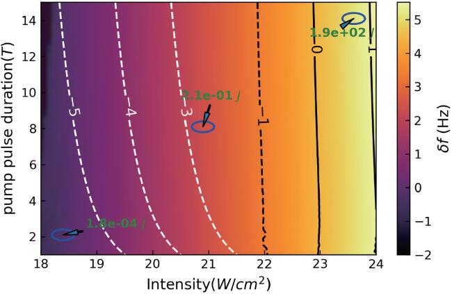
Figure 5. Frequency shift δf after a single collision at the optimal time offset by varying the pump laser intensity and pulse duration. The carrier frequency of the probe laser is set to be 3 × 10¹⁴ Hz (1 μm). White contour lines: shift of the comb teeth at the carrier frequency from equation ( |
We mainly discuss the experimental conditions in this section required for the signal detection given by equations (15 ), (16 ) and (21 ) respectively. For equations (15 ) and (16 ), because of the high repetition rate, the energy of a single pulse is limited to an order of 10−4 J (see the circle at the bottom left of figure 5). Here we assume the ultrafast laser can reach tens kilowatts average power [36]. For the equation (15 ), the direct contribution of the frequency rise term, we can see that the shift of the spectrum of the OFC is 0.3 Hz which is already larger than the 1mHz linewidth of some low-noise OFCs. So the requirement for the OFC is the original SNR is greater than ${\tilde{P}}_{\delta \omega }\approx 100\,{\rm{dB}}$. For the equation (16 ), the direct contribution of the change of TR, the corresponding shift of the comb teeth at the carrier frequency is about 10−5 Hz (plotted by white contour lines in figure 5). This places a higher demand on the linewidth of the OFC.
For the signal equation (21 ), obtained from the GPO variation, a single collision with a high peak intensity or multiple collisions at high repetition rate can achieve similar result. The black contour lines in figure 5 represent the shift of fCEO after single collision with a high peak intensity. If we adopt a realistic parameter 1023 W cm−2 [39], the shift δfCEO reaches order of Hz, surpassing the mHz linewidth by three orders of magnitude. Compared to the previous two signals, this demonstrates that the signal of the δfCEO is highly likely to be observed in the experiment.
4. Discussion and conclusion
In experiments, the utilized laser pulse always has a finite focal spot size. Then one has to check the validness of the simplification of equation (3 ) where the transverse gradient is neglected to facilitate our analysis. Qualitatively, in equation (4 ), ${{\rm{\nabla }}}_{\perp }{A}_{N}({\boldsymbol{x}},t)\propto {{\rm{\nabla }}}_{\perp }({E}_{\,\rm{pump}\,}^{2})$ indicates that the deflection of the photon near the central axis become nonnegligible when the transverse gradient of the pump field is relatively large: (1) the continuous increase in intensity caused by the inward convergence of light; (2) transverse spatial confinement, which, through the uncertainty principle, introduces a spread in the transverse momenta and hence a frequency shift in the axis [40]. Two simulations with focal spot size of 1 μm and 8 μm are conducted. The results are illustrated in figure 4(c). For both cases, the simulation results fit with our analysis quite well. In figure 4(b), we observe an unexpected increase which deviates from our theory. To explain this, we find that these deviations can be gradually eliminated when the focal spot of pump laser increases. For instance, the lower subplot of figure 4(c) shows the corresponding results when w0,pump = 8 μm. Figure 4(d) shows that when the waist of the pump laser increases, the simulation results quantitatively converge to the theoretical predictions.
The quantum-induced effect is small, its observation in simulations requires analyzing the evolution of scattered photons. In our simulations, this can be conveniently calculated by subtracting the electric field of the probe laser propagating in vacuum, Evac(x, t), from the electric field of the probe laser during the interaction, Eint(x, t). Escat = Eint(x, t) − Evac(x, t). Figures 6(a), (b) present the spatial distribution of Escat at different specific moments during the interaction process. The results indicate that the scattered light initially converges inward during the early stages and subsequently diffracts outward. More importantly, if we can establish a relationship between Eint and Escat, we can gain a clearer understanding of the role that the transverse effect can play. Assuming ${E}_{\,\rm{int}\,}({\boldsymbol{x}},t)=a({\boldsymbol{x}},t)\exp ({\rm{i}}({\theta }_{0}+{\theta }_{c})+{a}_{c})$, where θ0 = kx − ωt is the intrinsic vacuum phase evolution, and a(x, t) is the amplitude envelope, we have
$\begin{eqnarray}\begin{array}{rcl}{E}_{\,\rm{scat}\,} & = & {E}_{\rm{int}\,}-{E}_{\,\rm{vac}}\approx a({\boldsymbol{x}},t){{\rm{e}}}^{{\rm{i}}{\theta }_{0}}({\rm{i}}{\theta }_{c}+{\rm{i}}{\theta }_{c}{a}_{c}+{a}_{c})\\ & \approx & a({\boldsymbol{x}},t){{\rm{e}}}^{{\rm{i}}{\theta }_{0}}\cdot {\rm{i}}{\theta }_{c}\cdot {{\rm{e}}}^{{a}_{c}}\cdot {{\rm{e}}}^{-{\rm{i}}\frac{{a}_{c}}{{\theta }_{c}}}\\ & & \triangleq {\rm{i}}{a}^{{\prime} }({\boldsymbol{x}},t)\cdot {{\rm{e}}}^{{\rm{i}}({\theta }_{0}+{\alpha }^{{\prime} })}{\rm{.}}\end{array}\end{eqnarray}$
Here the relationship between Eint and Escat is determined by the envelope (${a}^{{\prime} }({\boldsymbol{x}},t)=a{\theta }_{c}^{{\prime} }=a\cdot {\theta }_{c}\cdot \exp ({a}_{c})$) and phase ($\exp ({\rm{i}}{\theta }_{0}+{\rm{i}}{\alpha }^{{\prime} })$) of Escat. This means that the envelope of the scattered light is related to the phase lag of Eint and ${\alpha }^{{\prime} }=-{a}_{c}/{\theta }_{c}$ means that the phase of the scattered light is closely related to the increase in intensity of Eint. Then, we substitute the form of Escat into the governing equation, ${{\rm{\nabla }}}^{2}E-{\partial }_{t}^{2}E={f}_{{\rm{corr}}}(\xi ,{{\boldsymbol{E}}}_{\,\rm{pump}\,},{{\boldsymbol{E}}}_{\,\rm{vac}\,})$, and have $\begin{eqnarray}\begin{array}{l}{\rm{i}}\left[{({\rm{\nabla }}({\theta }_{0}+{\alpha }^{^{\prime} }))}^{2}-{({\partial }_{t}({\theta }_{0}+{\alpha }^{^{\prime} }))}^{2}\right.\\ \quad -\,\left.\left(\displaystyle \frac{{\nabla }^{2}(a({\boldsymbol{x}},t){\theta }_{c}^{^{\prime} })}{a({\boldsymbol{x}},t){\theta }_{c}^{^{\prime} }}\right)+\left(\displaystyle \frac{{\partial }_{t}^{2}(a({\boldsymbol{x}},t){\theta }_{c}^{^{\prime} })}{a({\boldsymbol{x}},t){\theta }_{c}^{^{\prime} }}\right)\right]=0;\\ \quad \left[{\rm{\nabla }}\left(a\left({\boldsymbol{x}},t\right){\theta }_{c}^{^{\prime} }\right)\cdot {\rm{\nabla }}\left({\theta }_{0}+{\alpha }^{^{\prime} }\right)\right.\\ \quad -\,\left.{\partial }_{t}\left(a\left({\boldsymbol{x}},t\right){\theta }_{c}^{^{\prime} }\right)\cdot {\partial }_{t}\left({\theta }_{0}+{\alpha }^{^{\prime} }\right)\right]={f}_{\mathrm{corr}}\cdot {{\rm{e}}}^{-{\rm{i}}({\theta }_{0}+{\alpha }^{^{\prime} })}.\end{array}\end{eqnarray}$
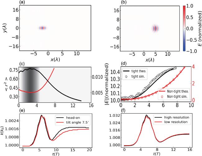
Figure 6. (a), (b) presents the spatial distribution of Escat at different time during the interaction process. (c) Red line presents the temporal evolution of $\langle {r}^{2}\rangle =\tfrac{\iint {r}^{2}{E}^{2}{{\rm{d}}}^{2}x}{\iint {E}^{2}{{\rm{d}}}^{2}x}$. Black line presents Δks calculated via $\frac{{{\rm{\nabla }}}_{\perp }^{2}\left(a\left({\boldsymbol{x}},t\right){\theta }_{c}^{{\prime} }\right)}{a\left({\boldsymbol{x}},t\right){\theta }_{c}^{{\prime} }}$. They exhibit a precise negative correlation. (d) After the corrections in equations ( |
While it is challenging to give an analytical solution, by considering the simulation results and an asymptotic form of the solution, the calculation can be significantly simplified. Firstly, the simulation results reveal that Escat exhibits a behavior analogous to the diffraction divergence of Gaussian light. Therefore, we introduce a description similar to the Gouy phase shift, ${\theta }_{0}+{\alpha }^{{\prime} }=({k}_{0}x-{\omega }_{0}t)+({\rm{\Delta }}{k}_{s}x)$ = k0(x − ct) + Δks(x − ct) + Δksct = (k0 + Δks)(ξ) + Δkscτ. Applying the paraxial approximation, the operator ∇2 is simplified to ${{\rm{\nabla }}}^{2}\to k{\partial }_{z}+{{\rm{\nabla }}}_{\perp }^{2}$. Secondly, by ignoring higher-order terms above ξ2, we can treat a(x, t) as $\exp (-{(x-ct)}^{2}/({\rm{\Delta }}{x}^{2}))$ to emphasize the primary physical process. With these approximations, equation (23 ) are reduced to 24 ) shows that when the transverse effect is nonzero, i.e. ${{\rm{\nabla }}}_{\perp }^{2}\left(a\left({\boldsymbol{x}},t\right){\theta }_{c}^{{\prime} }\right)/a\left({\boldsymbol{x}},t\right){\theta }_{c}^{{\prime} }\ne 0$, it leads a correction to the wave vector of the scattered light, Δks. We know that the intensity of Eint increases with ${\alpha }^{{\prime} }$, ${a}_{c}\,=-{\theta }_{c}(\tau )\cdot {\alpha }^{{\prime} }=-{\theta }_{c}(\tau )\cdot {\rm{\Delta }}{k}_{s}c\tau $. Thus, it explains the increase in intensity caused by the transverse effect, as the simulation results shown in figures 6(c), (d).
$\begin{eqnarray}2{k}_{0}({\rm{\Delta }}{k}_{s})=\left(\frac{{{\rm{\nabla }}}_{\perp }^{2}\left(a\left({\boldsymbol{x}},t\right){\theta }_{c}^{{\prime} }\right)}{a\left({\boldsymbol{x}},t\right){\theta }_{c}^{{\prime} }}\right){\rm{,}}\end{eqnarray}$
$\begin{eqnarray}2({\partial }_{\tau }{\theta }_{c}^{{\prime} }\cdot 2{k}_{0})={\theta }_{c}{{\rm{\nabla }}}^{2}({\theta }_{0}+{\alpha }^{{\prime} })+{f}_{{\rm{corr}}}\cdot {{\rm{e}}}^{-{\rm{i}}({\theta }_{0}+{\alpha }^{{\prime} })}{\rm{.}}\end{eqnarray}$
Equation (In equation (25 ), the two terms on the RHS of equation (25 ) will affect the phase ${\theta }_{c}^{{\prime} }$ of Eint. When the transverse effects are zero, it should revert to the one-dimensional case, i.e. the result obtained by the average variational approach. Since the transverse effects in equation (25 ) are mainly reflected in the term ${\theta }_{c}{{\rm{\nabla }}}^{2}({\theta }_{0}+{\alpha }^{{\prime} })$, the second term on the RHS of equation (25 ) should represent the phase lag caused by the ponderomotive force and the term ${\theta }_{c}{{\rm{\nabla }}}^{2}({\theta }_{0}+{\alpha }^{{\prime} })$ should correspond to the additional transverse correction to this phase. The calculated results indicate that the influence of this term is relatively minor, which ensures that our theoretical predictions of the spectrum remain reasonably accurate.
Another point is that, for simplicity, our previous analysis focused on the case of head-on collision. As shown in figure 1, the practical implementation of the proposed experimental setup may require the pump and probe lasers to collide at a small angle, due to constraints imposed by the cavity geometry. The reason for focusing on the case of head-on collisions lies in the typical parameters of the resonator, which is usually quite long. This results in angular tilts of less than 10∘, leading to only minor theoretical deviations. In addition, an analysis of our theory reveals that our setup is not sensitive to a small offset. As shown in figure 6(e), small angular offset does not affect the main results. Finally, to ensure the reliability of our simulations, we varied different parameters, including ξ, simulation resolution, and pump waist to confirm the convergence of the results. Some of the results are shown in figure 6(g).
In summary, we we proposed a novel scheme to measure and explore the effects of vacuum polarization, where a tightly-focused pump laser interacts with an OFC in its resonant cavity. An obvious frequency shift of the OFC pulse can be observed when it passes through the vacuum polarized by the ultraintense pump laser. Considering that OFC has ultrahigh frequency and time resolution, our scheme holds great potential in detecting the vacuum polarization.
Acknowledgments
This work is supported by the National Key R&D Program of China (Grant Nos. 2022YFA1603200, 2022YFA1603201, 2024YFA1613400), the National Natural Science Foundation of China (Grant Nos. 12135001, 11825502, 12075014, 12475243), the Strategic Priority Research Program of the Chinese Academy of Sciences (Grant No. XDA25050900), the Science and Technology on Plasma Physics Laboratory (Grant No. 6142A04210110). BQ acknowledges support from the National Natural Science Funds for Distinguished Young Scholars (Grant No. 11825502). The authors gratefully acknowledge that the computing time is provided by the Tianhe-2 supercomputer at the National Supercomputer Center in Guangzhou.
Conflict of interest
The authors have no conflicts to disclose.
Data availability
The data that support the findings of this study are available from the corresponding author upon reasonable request.
Appendix A Averaged Lagrangian
To carry out our analysis, we first follow the procedure outlined in [27]. As mentioned above, we introduce the following average Lagrangian with A = Φ(θ, x, t), Φ is a periodic function of θ, and the laser configuration mentioned in equation (3 ).
$\begin{eqnarray}\begin{array}{rcl}\bar{{ \mathcal L }} & = & \iint \frac{1}{2\pi }{\displaystyle \int }_{\theta =0}^{2\pi }{ \mathcal L }({{\rm{\partial }}}_{t}A,{{\rm{\partial }}}_{x}A,A)\,{\rm{d}}\theta \,{\rm{d}}x{\rm{d}}t\\ & = & \iint \frac{1}{2\pi }{\displaystyle \int }_{\theta =0}^{2\pi }{ \mathcal L }(-\omega {{\rm{\Phi }}}_{\theta }+{{\rm{\Phi }}}_{t},k{{\rm{\Phi }}}_{\theta }+{{\rm{\Phi }}}_{x},{\rm{\Phi }})\,{\rm{d}}\theta \,{\rm{d}}x{\rm{d}}t.\end{array}\end{eqnarray}$
We ignore the transverse gradient effect for now. The equations from the variational principle applied to this average Lagrangian, i.e. ${\delta }_{{\rm{\Phi }}}\bar{{ \mathcal L }}=0$ (regarding the three variables θ, x, t as mutually independent), is equivalent to the E–L equation derived from the original Lagrangian ${ \mathcal L }$. A careful proof of it can be found in the literature [27]. Then, if we can find a way that the integral $\bar{{\mathscr{L}}}={\int }_{\theta =0}^{2\pi }{ \mathcal L }({\partial }_{t}A,{\partial }_{x}A,A){\rm{d}}\theta $ can be executed analytically or approximately, we have $\bar{{ \mathcal L }}=\iint \bar{{\mathscr{L}}}(x,t,\omega ,k,a){\rm{d}}x{\rm{d}}t$. Consequently, variations for δΦ will transform the E–L equations into equations involving modulation parameters ω, k, a. Here, a denotes the introduced integral parameter which is usually associated with the wavetrain amplitude. It can also be shown that the condition A is a periodic function of θ is equivalent to the variational equation ${\delta }_{\theta }\bar{{ \mathcal L }}=\delta \iint \bar{{\mathscr{L}}}(x,t,{\partial }_{x}\theta ,-{\partial }_{t}\theta ,a)\,{\rm{d}}x{\rm{d}}t=0$. These two equations together constitute the complete governing equation for the modulated wavetrain.Next we need to choose the appropriate form of the wavetrain A, which is also the key to use this method. The selection of the corresponding wavetrain should follow two principles, the integration is easy to perform (allowing proper approximation) and the physics corresponding to the approximation is sufficiently clear. For example, the assumption we have chosen here is $A(x,t)=(a+{a}_{1})\cos (\theta +{\theta }_{1})$, a result that takes into account the fact that the main fluctuations and modulations are centred in the elastic scattering region and includes the possible contribution of the high-frequency interaction term. It should be noted here that since we are concerned with the results under near-field conditions, the solution during the interaction does not need to satisfy the on-shell condition. So in this case, we do not just remove the high frequency oscillation term as previous literature [32]. Otherwise, if the form $A(x,t)=a(x,t)\cos (\theta )$ is used directly, the modulating component of the high-frequency oscillation is hidden (see results shown in the figure 2).
Substitute $A(x,t)=(a+{a}_{1})\cos (\theta +{\theta }_{1})$ into equation (2 ), where ${a}_{1}=\,\rm{Re}\,[\tilde{a}\exp ({\rm{i}}{\rm{\Theta }})],{\theta }_{1}=\,\rm{Re}\,[\tilde{\theta }\exp ({\rm{i}}{\rm{\Theta }})]$ and $\exp ({\rm{i}}{\rm{\Theta }})=\exp ({\rm{i}}Kx-{\rm{i}}{\rm{\Omega }}t)$ is the oscillation term of the pump laser. Integrate θ and Θ from 0 to 2π to obtain the average Lagrangian 3 ). Finally, using the variational principle for variations in a, we can obtain dispersion relation equation (A.3 ).
$\begin{eqnarray}\begin{array}{rcl}{ \mathcal L } & = & -\,\frac{1}{4}{a}^{2}\left({k}^{2}-{\omega }^{2}+{\tilde{k}}^{2}-{\tilde{\omega }}^{2}+\frac{1}{2}{A}_{N}({k}^{2}+{\omega }^{2}+2k\omega )\right)\\ & & -\frac{1}{4}{a}^{2}\left(\frac{1}{2}{\tilde{A}}_{N}(2k\tilde{k}+2\omega \tilde{\omega }+2\tilde{k}w+2k\tilde{\omega })\right)\\ & & -\frac{1}{4}2a\tilde{a}\left(2k\tilde{k}-2\omega \tilde{\omega }+\frac{1}{2}{\tilde{A}}_{N}({k}^{2}+2k\omega +{\omega }^{2})\right)\\ & & -\frac{1}{8}({A}_{N})({({\partial }_{x}a)}^{2}-2{\partial }_{t}a{\partial }_{x}a+{({\partial }_{x}a)}^{2})\\ & & -\frac{1}{8}({\tilde{A}}_{N})({\partial }_{x}a{\partial }_{x}\tilde{a}-2{\partial }_{t}a{\partial }_{x}\tilde{a}-2{\partial }_{t}\tilde{a}{\partial }_{x}a+{\partial }_{x}a{\partial }_{x}\tilde{a}).\end{array}\end{eqnarray}$
We then use the relation from $\delta \bar{{ \mathcal L }}/\delta \tilde{a}=0\to \tilde{\omega }\,+\tilde{{A}_{N}}k-\tilde{k}=0$. Ignoring terms of magnitude $O({A}_{N}^{2})$, we can finally get equation ( $\begin{eqnarray}\begin{array}{l}\frac{1}{2}a\left(-{k}^{2}+{\omega }^{2}-\frac{1}{2}{A}_{N}{k}^{2}-{A}_{N}k\omega -\frac{1}{2}{A}_{N}{\omega }^{2}\right)\\ +\,\frac{1}{2}(-{\partial }_{x}{\partial }_{x}a+{\partial }_{t}{\partial }_{t}a)\\ +\,\frac{1}{4}\left[({\partial }_{x}-{\partial }_{t})({A}_{N}{\partial }_{t}a-{A}_{N}{\partial }_{x}a)\right]=0{\rm{.}}\end{array}\end{eqnarray}$
In order to make the main text appear more concise, we do not consider in the main text the additional contribution formed by the tight focusing nature of the probe laser, i.e. the $\frac{1}{2}(-{\partial }_{x}{\partial }_{x}a+{\partial }_{t}{\partial }_{t}a)$ term. Although this may be important in some cases.
Appendix B Benchmark
Using the H–E Lagrangian and the principle of least action, we can obtain a modified version of Maxwell’s equations that takes into account the quantum vacuum effect. It is similar to Maxwell’s equations in the medium, the only difference is the expressions of polarization, P, and magnetization, M, see equation (B.1 ). Our simulations are based on this vacuum-polarization-corrected Maxwell’s equations. We used the algorithm proposed by T. Grismayer [28] (modified algorithm based on standard Ye scheme) and added the corresponding module to the PIC program EPOCH.
$\begin{eqnarray}\begin{array}{rcl}{\boldsymbol{P}} & = & \frac{\partial {{ \mathcal L }}_{{\rm{HE}}}}{\partial {\boldsymbol{E}}}=2\xi \left[2\left({{\boldsymbol{E}}}^{2}-{{\boldsymbol{B}}}^{2}\right){\boldsymbol{E}}+7({\boldsymbol{E}}\cdot {\boldsymbol{B}}){\boldsymbol{B}}\right]{\rm{;}}\\ {\boldsymbol{M}} & = & \frac{\partial {{ \mathcal L }}_{{\rm{HE}}}}{\partial {\boldsymbol{B}}}=-2\xi \left[2\left({{\boldsymbol{E}}}^{2}-{{\boldsymbol{B}}}^{2}\right){\boldsymbol{B}}-7({\boldsymbol{E}}\cdot {\boldsymbol{B}}){\boldsymbol{E}}\right]{\rm{.}}\end{array}\end{eqnarray}$
We start from an idealized scenario that considers the interaction between a probe laser and a sinusoidal electromagnetic field, as illustrated in figure 7. At this point, equation (4 ) will degenerate into the most basic withham equations (similar to J. T. Mendonça’s work, photon can be accelerated (frequency upshift)) $\dot{x}=\partial \omega (t,x,k)/\partial k,\dot{k}=-\partial \omega (t,x,k)/\partial x$, ω is the effective dispersion relation of the probe laser. The primary simulation results are depicted in figures 7(b)–(e), which validate the theory for trajectory evolution $\dot{x}=cn$, wave-vector evolution $\dot{k}$, local dispersion relation approximation and etc. These simulations not only serve as theoretical verification, but also provide support for the rationality of the following operations used in our simulations. Firstly, the background electromagnetic field has been manually provided at each time step and does not participate in the evolution of the electromagnetic field. Its role is to polarize the vacuum. Because of aprobe ≪ apump, such an operation should be appropriate. Secondly, to demonstrate the vacuum polarization effect within a limited simulation time, we have artificially increased the nonlinear parameter ξ in equation (B.1 ) to 4.3 × 10−45 (see also in [28]). The physical significance of the results remains unaffected by this. Instead, it is merely a proportional adjustment of a constant aimed at emphasizing the effects with greater clarity. This is because the real physical parameter ξ is very small, the effect of vacuum polarization can only consider the part that is proportional to ξ. As in figures 7(b), (c), after ξ is reduced by 5 times, the frequency growth rate is reduced by 5 times, which provides great convenience for us to rescale the simulation back to real-world physics to obtain explicit values. It is necessary to ensure that the physical process remains unchanged, which requires ξE2 ≪ 1. So ξ is chosen to make ξE2 between 1 × 10⁻⁴ and 1 × 10⁻² in the simulations.
Figure 7. 2D simulation results: a probe Gaussian laser with peak intensity Iprobe = 1.37 × 10²⁰ W cm−2(a = 10), wavelength λ = 1 μm, gaussian temporal profile with duration Δτ = 5T and focal radius rprobe = 5λ is incident from the left boundary into a 100λ × 50λ simulation box (along the X axis). At a time of 10T, a sinusoidal electromagnetic field with an amplitude of a = 1000 appears, where ${E}_{y}=\sin ({\lambda }_{b}x),{B}_{z}=-\sin ({\lambda }_{b}x),{\lambda }_{b}=100{\lambda }_{0}$. As the sinusoidal background electromagnetic field moves with the probe light at the speed of light in the same direction, the probe laser is almost always at the initial given phase of the background field. It should be noted that our program allows to manually set the pump field at each time step. Here we changed the direction of the pump laser’s magnetic field, so that the vacuum polarization effect exists (Lorentz invariant is not zero). Conversely, in realistic scenarios the vacuum polarization effect does not exist when pump laser and probe laser propagate in the same direction(lorentz invariant is zero). This artificial adjustment was made to simulate an idealized case, serving as a benchmark for the program. (a) The probe laser is on the rising edge of the pump laser and is accelerated. Where the red and blue pulse are two-dimensional spatial intensity distribution of the probe laser. (b), (c) The time evolution of the position and wave vector of the probe laser respectively. Solid lines are theoretical predictions, and dots represent simulation results. (d) Dispersion relation in evolution. (e) Change the wavelength of the pump laser, and the wave-vector growth of the probe laser at 60T. |