


1. Introduction
Solitons are stable waveforms in nonlinear systems with extensive physical applications. They play a significant role in fields such as optical fiber communications, plasma physics, condensed matter physics, fluid dynamics, and quantum field theory [1-7]. Among the various types of solitons, nondegenerate solitons represent a unique class of solitary waves capable of describing distinct polarization states in multi-channel optical fiber systems. The term ‘nondegenerate' indicates that the intensity profiles of different components within a coupled system can exhibit various structures, including single-hump, double-hump, or flat-top profiles [8]. This concept has subsequently evolved to include the idea that individual components display different wavenumbers [9].
In recent years, researchers have utilized the Hirota bilinear method, Kadomtsev-Petviashvili hierarchy reduction, and the Darboux transformation to derive nondegenerate soliton solutions for a range of systems, including various types of coupled nonlinear Schrödinger equations, the Manakov system, and the Fokas-Lenells system [10-22]. Moreover, the classification of nondegenerate solitons has expanded to include not only bright solitons but also other forms, such as nondegenerate dark solitons, breathers, and rogue waves [18-24]. These advancements underscore the ubiquity and diversity of nondegenerate solitons, as well as their critical role in advancing the understanding of nonlinear wave dynamics [10-12].
Previous studies on nondegenerate solitons have primarily focused on (1+1)-dimensional coupled systems. However, (2+1)-dimensional coupled systems, with higher spatial dimensions, are expected to exhibit a broader range of nondegenerate soliton solutions. To expand the variety of these solutions and enable them to describe more complex nonlinear phenomena, this paper explores a (2+1)-dimensional coupled system, resulting in the derivation of a novel nondegenerate soliton solution via the Hirota bilinear method [25-27]. Since the function of the variable y in this solution can be chosen arbitrarily, selecting different types of functions allows for the construction of numerous nondegenerate solitons with various waveforms, as well as control over their shapes.
The structure of the paper is as follows. In section 2 , the Hirota bilinear method is used to solve the equation, followed by application of the Gram determinant [28,29] to express the general nondegenerate N-soliton solution of the system. In section 3 , we select various functional forms to obtain single, double, and triple nondegenerate soliton solutions, demonstrating a range of distinct waveforms. Finally, the key findings of the study are summarized in section 4 .
2. General nondegenerate N-soliton solution
The (2+1)-dimensional three-component long-wave-short-wave resonant interaction system is given as follows [30]
$\begin{eqnarray}\begin{array}{rcl}{\rm{i}}{U}_{t}+{U}_{xx}+UW & =& 0,\\ {\rm{i}}{V}_{t}+{V}_{xx}+VW & =& 0,\\ {W}_{t}+{W}_{y}+{\left(| U{| }^{2}+| V{| }^{2}\right)}_{x} & =& 0,\end{array}\end{eqnarray}$
where U and V are complex functions representing the short-wave components, and W is a real function describing the long-wave component. This system is integrable and has been derived using the asymptotically exact reduction method, which is based on Fourier expansion and spatio-temporal rescaling, from the Kadomtsev-Petviashvili equation [31]. It can be employed to describe two-dimensional nonlinear waves in various fields [32-34]. For instance, in the study of water wave behavior, the short-wave components U and V represent high-frequency small-scale waves on the water surface, such as ripples and small waves, or rapid local disturbances induced by wind and other factors. In contrast, the long-wave component W corresponds to low-frequency, large-scale wave motions, typically manifested as ocean waves, storm surges, or tsunamis. The nonlinear coupling between the components U, V, and W can lead to complex wave phenomena, generating solitons and other nonlinear wave modes. On the other hand, in optical systems, components U and V represent rapidly changing light fields, capable of describing high-frequency oscillations, phase shifts, and other rapid variations of light waves. The component W represents the low-frequency part of the light field, primarily describing the overall propagation characteristics of the light wave, slow variations in wave behavior, and large-scale light field structures. In recent years, several types of soliton solutions such as rogue waves, breathers, and lumps have been discovered for this system [35-40]. Furthermore, in [41], by selecting exponential functions as seed solutions, solitoff-type and X-type nondegenerate solitons were obtained. It was also revealed through asymptotic analysis that the collision types between the nondegenerate solitons and degenerate solitons of different components are distinct.In order to solve equation (1 ), we apply the transformations U=g/f, V=h/f and $W=2{(\mathrm{ln}f)}_{xx}$. The Hirota bilinear forms of equation (1 ) can be written as 3 ) into equation (2 ) and collect all the coefficients of ϵi(where i=1, 2, ⋅ s). Then, set these coefficients to zero. For ϵ1, we have
$\begin{eqnarray}\begin{array}{rcl}\left({D}_{x}^{2}+{\rm{i}}{D}_{t}\right)g\cdot f & =& 0,\\ \left({D}_{x}^{2}+{\rm{i}}{D}_{t}\right)h\cdot f & =& 0,\\ \left({D}_{x}{D}_{y}+{D}_{x}{D}_{t}+\lambda \right)f\cdot f+g\cdot {g}^{* }+h\cdot {h}^{* } & =& 0,\end{array}\end{eqnarray}$
where Dx, Dy, and Dt are the bilinear operators, the symbol ‘*' represents complex conjugation, and λ is an arbitrary constant. For simplification of calculations, we set λ=0. To derive the nondegenerate N-soliton solution for the system, we expand g, h, and f in the following series forms $\begin{eqnarray}\begin{array}{rcl}g & =& \varepsilon {g}_{1}+{\varepsilon }^{3}{g}_{3}+\cdot s+{\varepsilon }^{4N-1}{g}_{4N-1},\\ h & =& \varepsilon {h}_{1}+{\varepsilon }^{3}{h}_{3}+\cdot s+{\varepsilon }^{4N-1}{h}_{4N-1},\\ f & =& 1+{\varepsilon }^{2}{f}_{2}+{\varepsilon }^{4}{f}_{4}+\cdot s+{\varepsilon }^{4N}{f}_{4N}.\end{array}\end{eqnarray}$
Substitute equation ( $\begin{eqnarray}{\rm{i}}{g}_{1t}+{g}_{1xx}=0,\end{eqnarray}$
$\begin{eqnarray}{\rm{i}}{h}_{1t}+{h}_{1xx}=0.\end{eqnarray}$
Since the two equations mentioned above are linear partial differential equations with respect to the variables x and t, their solutions can be expressed as linear superpositions of N distinct exponential functions when constructing N-soliton solutions. The variables x and t are combined into linear functions and incorporated into the exponents of the exponential functions. Additionally, the coefficients of each exponential function are defined as arbitrary functions of the variable y, which effectively separates y from x and t. As a result, the expressions for g1 and h1 are given by 6 ) that g1 and h1 each comprise N arbitrary functions of y. The parameters kj and ml are complex constants. Inserting equation (6 ) into the coefficient of ϵ2, we obtain
$\begin{eqnarray}\begin{array}{rcl}{g}_{1} & =& \displaystyle \sum _{j=1}^{N}{p}_{j}(y){{\rm{e}}}^{{\eta }_{j}},\\ {h}_{1} & =& \displaystyle \sum _{l=1}^{N}{q}_{l}(y){{\rm{e}}}^{{\xi }_{l}}.\end{array}\end{eqnarray}$
Here, pj(y) and ql(y) are arbitrary functions of y, and the variables ηj and ξl are defined as ${\eta }_{j}={k}_{j}x+{\rm{i}}{k}_{j}^{2}t$ and ${\xi }_{l}={m}_{l}x+{\rm{i}}{m}_{l}^{2}t$, respectively. As a result, it follows from equation ( $\begin{eqnarray}2{f}_{2xy}+2{f}_{2xt}+\displaystyle \sum _{j,l=1}^{N}\left({p}_{j}(y){p}_{l}^{* }(y){{\rm{e}}}^{{\eta }_{j}+{\eta }_{l}^{* }}+{q}_{j}(y){q}_{l}^{* }(y){{\rm{e}}}^{{\xi }_{j}+{\xi }_{l}^{* }}\right)=0,\end{eqnarray}$
subsequently, solving the above equation yields $\begin{eqnarray}\begin{array}{rcl}{f}_{2} & =& \displaystyle \sum _{j,l=1}^{N}\left({a}_{jl}(y){{\rm{e}}}^{{\eta }_{j}+{\eta }_{l}^{* }}+{b}_{jl}(y){{\rm{e}}}^{{\xi }_{j}+{\xi }_{l}^{* }}\right),\\ {a}_{jl}(y) & =& \left({c}_{jl}-\displaystyle \int \frac{{p}_{j}(y){p}_{l}^{* }(y)}{2\left({k}_{j}+{k}_{l}^{* }\right)}{{\rm{e}}}^{{\rm{i}}\left({k}_{j}^{2}-{k}_{l}^{* 2}\right)y}{\rm{d}}y\right){{\rm{e}}}^{-{\rm{i}}\left({k}_{j}^{2}-{k}_{l}^{* 2}\right)y},\\ {b}_{jl}(y) & =& \left({c}_{jl}^{{\prime} }-\displaystyle \int \frac{{q}_{j}(y){q}_{l}^{* }(y)}{2\left({m}_{j}+{m}_{{\rm{l}}}^{* }\right)}{{\rm{e}}}^{{\rm{i}}\left({m}_{j}^{2}-{m}_{l}^{* 2}\right)y}{\rm{d}}y\right){{\rm{e}}}^{-{\rm{i}}\left({m}_{j}^{2}-{m}_{l}^{* 2}\right)y},\end{array}\end{eqnarray}$
where cjl and ${c}_{jl}^{{\prime} }$ are constants of integration. The coefficients for ϵ3 and ϵ4 are then given by the following expressions. $\begin{eqnarray}{\rm{i}}{g}_{3t}+{g}_{3xx}+{\rm{i}}{g}_{1t}{f}_{2}-{\rm{i}}{g}_{1}{f}_{2t}+{f}_{2}{g}_{1xx}+{g}_{1}{f}_{2xx}-2{g}_{1x}{f}_{2x}=0,\end{eqnarray}$
$\begin{eqnarray}{\rm{i}}{h}_{3t}+{h}_{3xx}+{\rm{i}}{h}_{1t}{f}_{2}-{\rm{i}}{h}_{1}{f}_{2t}+{f}_{2}{h}_{1xx}+{h}_{1}{f}_{2xx}-2{h}_{1x}{f}_{2x}=0,\end{eqnarray}$
$\begin{eqnarray}\begin{array}{l}2\left({f}_{4xy}+{f}_{4xt}+{f}_{2}{f}_{xy}+{f}_{2}{f}_{2xt}-{f}_{2x}{f}_{2y}-{f}_{2x}{f}_{2t}\right)\\ \quad +{g}_{1}{g}_{3}^{* }+{g}_{3}{g}_{1}^{* }+{h}_{1}{h}_{3}^{* }+{h}_{3}{h}_{1}^{* }=0.\end{array}\end{eqnarray}$
Substituting equation (6 ) and equation (8 ) into the above three equations and solving them results in the following outcome 3 ). This solution can be clearly expressed using the compact and convenient Gram determinants 14 ), T and I represent the transpose operator and the 2N-order identity matrix, respectively. In equation (15 ), H and 0 denote the conjugate transpose operator and the N-order zero matrix, respectively.
$\begin{aligned}g_{3}(y)= & \sum_{j, l, r=1}^{N} \Delta_{j l r}(y) \mathrm{e}^{\eta_{j}+\xi_{l}+\xi_{r}^{*}}+\sum_{\substack{j, l=1 \\j \neq l}}^{N} \Gamma_{j l l}(y) \mathrm{e}^{\eta_{j}+\eta_{l}+\eta_{l}^{*}} \\& +\sum_{\substack{j, l, r=1 \\j \neq l \neq r, j<l}}^{N} \Gamma_{j l r}(y) \mathrm{e}^{\eta_{j}+\eta_{l}+n_{r}^{*}} \\h_{3}(y)= & \sum_{j, l, r=1}^{N} \Theta_{j l r}(y) \mathrm{e}^{\xi_{j}+\eta_{l}+\eta_{r}^{*}}+\sum_{\substack{j, l=1 \\j \neq l}}^{N} \Lambda_{j l l}(y) \mathrm{e}^{\xi_{j}+\xi_{l}+\xi_{l}^{*}}\\& +\sum_{\substack{j, l, r=1 \\j \neq l \neq r, j<l}}^{N} \Lambda_{j l r}(y) \mathrm{e}^{\xi_{j}+\xi_{l}+\xi_{r}^{*}} \\f_{4}(y)= & \sum_{\substack{j, l, r, s=1 \\N}}^{N} \Omega_{j l r s}(y) \mathrm{e}^{\eta_{j}+\eta_{l}^{*}+\xi_{r}+\xi_{s}^{*}} \\& +\sum_{\substack{j, l=1 \\j<l}}^{N}\left(\Psi_{j j l l}(y) \mathrm{e}^{\eta_{j}+\eta_{j}^{*}+\eta_{l}+\eta_{l}^{*}}+\Phi_{j j l l}(y) \mathrm{e}^{\xi_{j}+\xi_{j}^{*}+\xi_{l}+\xi_{l}^{*}}\right)\\+ & \sum_{\substack{j, l, r=1 \\j \neq l \neq r}}^{N}\left(\Psi_{j j l r}(y) \mathrm{e}^{\eta_{j}+\eta_{j}^{*}+\eta_{l}+\eta_{r}^{*}}\right. \\+ & \left.\Phi_{j j l r}(y) \mathrm{e}^{\xi_{j}+\xi_{j}^{*}+\xi_{l}+\xi_{r}^{*}}\right) \\+ & \sum_{\substack{j, l, r, s=1 \\j \neq l \neq r \neq s \\j<l, r<s}}^{N}\left(\Psi_{j l r s}(y) \mathrm{e}^{\eta_{j}+\eta_{l}+\eta_{r}^{*}+\eta_{s}^{*}}\right. \\+ & \left.\Phi_{j l r s}(y) \mathrm{e}^{\xi_{j}+\xi_{l}+\xi_{r}^{*}+\xi_{s}^{*}}\right),\end{aligned}$
where $\begin{eqnarray}\begin{array}{rcl}{{\rm{\Delta }}}_{jlr}(y) & =& \frac{{b}_{rl}(y){p}_{j}(y)\left({k}_{j}-{m}_{l}\right)}{{k}_{j}+{m}_{r}^{* }},\\ {{\rm{\Gamma }}}_{\alpha \beta \gamma }(y) & =& \left({k}_{\alpha }-{k}_{\beta }\right)\cdot \left[\frac{{p}_{\alpha }(y){a}_{\gamma \beta }(y)}{{k}_{\alpha }+{k}_{\gamma }^{* }}-\frac{{p}_{\beta }(y){a}_{\gamma \alpha }(y)}{{k}_{\beta }+{k}_{\gamma }^{* }}\right],\\ {{\rm{\Theta }}}_{jlr}(y) & =& \frac{{a}_{rl}(y){q}_{j}(y)\left({m}_{j}-{k}_{l}\right)}{{m}_{j}+{k}_{r}^{* }},\\ {{\rm{\Lambda }}}_{\alpha \beta \gamma }(y) & =& \left({m}_{\alpha }-{m}_{\beta }\right)\cdot \left[\frac{{q}_{\alpha }(y){b}_{\gamma \beta }(y)}{{m}_{\alpha }+{m}_{\gamma }^{* }}-\frac{{q}_{\beta }(y){b}_{\gamma \alpha }(y)}{{m}_{\beta }+{m}_{\gamma }^{* }}\right],\\ {{\rm{\Omega }}}_{jlrs}(y) & =& {a}_{lj}(y){b}_{sr}(y)\frac{\left({k}_{j}-{m}_{r}\right)\left({k}_{l}^{* }-{m}_{s}^{* }\right)}{\left({k}_{j}+{m}_{s}^{* }\right)\left({m}_{r}+{k}_{l}^{* }\right)},\\ {{\rm{\Psi }}}_{\alpha \beta \gamma \delta }(y) & =& \left({k}_{\alpha }-{k}_{\gamma }\right)\left({k}_{\beta }^{* }-{k}_{\delta }^{* }\right)\\ & & \cdot \left[\frac{{a}_{\beta \alpha }(y){a}_{\delta \gamma }(y)}{\left({k}_{\alpha }+{k}_{\delta }^{* }\right)\left({k}_{\gamma }+{k}_{\beta }^{* }\right)}-\frac{{a}_{\delta \alpha }(y){a}_{\beta \gamma }(y)}{\left({k}_{\alpha }+{k}_{\beta }^{* }\right)\left({k}_{\gamma }+{k}_{\delta }^{* }\right)}\right],\\ {{\rm{\Phi }}}_{\alpha \beta \gamma \delta }(y) & =& \left({m}_{\alpha }-{m}_{\gamma }\right)\left({m}_{\beta }^{* }-{m}_{\delta }^{* }\right)\\ & & \cdot \left[\frac{{b}_{\beta \alpha }(y){b}_{\delta \gamma }(y)}{\left({m}_{\alpha }+{m}_{\delta }^{* }\right)\left({m}_{\gamma }+{m}_{\beta }^{* }\right)}-\frac{{b}_{\delta \alpha }(y){b}_{\beta \gamma }(y)}{\left({m}_{\alpha }+{m}_{\beta }^{* }\right)\left({m}_{\gamma }+{m}_{\delta }^{* }\right)}\right].\end{array}\end{eqnarray}$
Similarly, additional expressions for gj, hj, and fl can be derived by solving the coefficient equations for higher powers of ϵ. Ultimately, the general nondegenerate N-soliton solution of the system is obtained by setting ϵ=1 in equation ( $\begin{array}{l}U=\frac{g}{f}=\frac{\left|\begin{array}{ccc}A & I & \phi \\-I & B & 0^{\mathrm{T}} \\0^{\prime} & C_{1} & 0\end{array}\right|}{\left|\begin{array}{cc}A & I \\-I & B\end{array}\right|}, \quad V=\frac{h}{f}=\frac{\left|\begin{array}{ccc}A & I & \phi \\-I & B & 0^{\mathrm{T}} \\0^{\prime} & C_{2} & 0\end{array}\right|}{\left|\begin{array}{cc}A & I \\-I & B\end{array}\right|}, \\W=2(\ln f)_{x x}=2\left[\ln \left(\left|\begin{array}{cc}A & I \\-I & B\end{array}\right|\right)\right]_{x x},\end{array}$
where $\begin{eqnarray}\displaystyle \begin{array}{rcl}A & =& \left(\begin{array}{cc}{A}_{j{j}^{{\prime} }} & {A}_{jl}\\ {A}_{jl}^{H} & {A}_{l{l}^{{\prime} }}\end{array}\right),\,B=\left(\begin{array}{cc}{B}_{j{j}^{{\prime} }} & {\bf{0}}\\ {\bf{0}} & {B}_{l{l}^{{\prime} }}\end{array}\right),\\ {A}_{j{j}^{{\prime} }} & =& \frac{{{\rm{e}}}^{{\eta }_{j}+{\eta }_{{j}^{{\prime} }}^{* }}}{{k}_{j}+{k}_{{j}^{{\prime} }}^{* }},{A}_{l{l}^{{\prime} }}=\frac{{{\rm{e}}}^{{\xi }_{l}+{\xi }_{{l}^{{\prime} }}^{* }}}{{m}_{l}+{m}_{{l}^{{\prime} }}^{* }},{A}_{jl}=\frac{{{\rm{e}}}^{{\eta }_{j}+{\xi }_{l}^{* }}}{{k}_{j}+{m}_{l}^{* }},\\ {B}_{j{j}^{{\prime} }} & =& {a}_{{j}^{{\prime} }j}(y)\left({k}_{j}^{* }+{k}_{{j}^{{\prime} }}\right),{B}_{l{l}^{{\prime} }}={b}_{{l}^{{\prime} }l}(y)\left({m}_{l}^{* }+{m}_{{l}^{{\prime} }}\right),\\ {C}_{1} & =& -({p}_{1}(y),{p}_{2}(y),\,\ldots ,{p}_{N}(y),\mathop{\overbrace{0,0,\ldots ,0}}\limits^{N}),\\ {C}_{2} & =& -(\mathop{\overbrace{0,0,\ldots ,0}}\limits^{N},{q}_{1}(y),{q}_{2}(y),\,\ldots ,\,{q}_{N}(y)),\\ \phi & =& {\left({{\rm{e}}}^{{\eta }_{1}},{{\rm{e}}}^{{\eta }_{2}},\,\ldots ,\,{{\rm{e}}}^{{\eta }_{N}},{{\rm{e}}}^{{\xi }_{1}},{{\rm{e}}}^{{\xi }_{2}},\,\ldots ,\,{{\rm{e}}}^{{\xi }_{N}}\right)}^{{\rm{T}}},\\ {{\bf{0}}}^{{\prime} } & =& (\mathop{\overbrace{0,0,\ldots ,0}}\limits^{2N}),\\ {a}_{{j}^{{\prime} }j}(y) & =& \left({c}_{{j}^{{\prime} }j}-\displaystyle \int \frac{{p}_{{j}^{{\prime} }}(y){p}_{j}^{* }(y)}{2\left({k}_{{j}^{{\prime} }}+{k}_{j}^{* }\right)}{{\rm{e}}}^{{\rm{i}}\left({k}_{{j}^{{\prime} }}^{2}-{k}_{j}^{* 2}\right)y}{\rm{d}}y\right)\\ & & \times {{\rm{e}}}^{-{\rm{i}}\left({k}_{{j}^{{\prime} }}^{2}-{k}_{j}^{* 2}\right)y},\\ {b}_{{l}^{{\prime} }l}(y) & =& \left({c}_{{l}^{{\prime} }l}^{{\prime} }-\displaystyle \int \frac{{q}_{{l}^{{\prime} }}(y){q}_{l}^{* }(y)}{2\left({m}_{{l}^{{\prime} }}+{m}_{l}^{* }\right)}{{\rm{e}}}^{{\rm{i}}\left({m}_{{l}^{{\prime} }}^{2}-{m}_{l}^{* 2}\right)y}{\rm{d}}y\right)\\ & & \times {{\rm{e}}}^{-{\rm{i}}\left({m}_{{l}^{{\prime} }}^{2}-{m}_{l}^{* 2}\right)y},\\ {c}_{{j}^{{\prime} }j} & =& {c}_{j{j}^{{\prime} }}^{* },{c}_{{l}^{{\prime} }l}^{{\prime} }={c}_{l{l}^{{\prime} }}^{{\prime} * },\quad j,{j}^{{\prime} },l,{l}^{{\prime} }=1,2,\,\ldots ,\,N,\\ {\eta }_{r} & =& {k}_{r}x+{\rm{i}}{k}_{r}^{2}t,{\xi }_{r}={m}_{r}x+{\rm{i}}{m}_{r}^{2}t.\end{array}\end{eqnarray}$
In equation (3. Novel types of nondegenerate solitons
To clarify the structures and interactions of novel nondegenerate solitons, we present a series of illustrative figures below.
Firstly, setting N=1 in equations (14 ) and (15 ) yields the general nondegenerate one-soliton solution of the system.16 ) and (17 ), it can be observed that the propagation velocities of the nondegenerate single solitons for the components U and V are 2m1I and 2k1I, respectively, while their waveforms are primarily controlled by p1(y) and q1(y). By selecting the Fourier series expansions for the pulse wave and the triangular wave as ${p}_{1}(y)=2/3+\frac{4}{\pi }{\sum }_{n=1}^{90}[\sin (n\pi /3)\cdot \cos (2n\pi y/3)/n]$ and ${q}_{1}(y)=\frac{16}{{\pi }^{2}}{\sum }_{n=1}^{90}\left[{(-1)}^{n-1}\cdot \sin (2(2n-1)\pi y/3)\right.$ $\left./{(2n-1)}^{2}\right]$, a nondegenerate one-soliton can be represented, demonstrating the corresponding waveform in the y-direction, as shown in figure 1.
$\begin{eqnarray}\begin{array}{rcl}U & =& \frac{{p}_{1}(y){{\rm{e}}}^{{\rm{i}}{\eta }_{1I}-\frac{\alpha (y)}{2}}\cosh \left({\xi }_{1R}+\frac{\beta (y)+{\phi }_{2}}{2}\right)}{{\gamma }_{1}\cosh \left({\eta }_{1R}+{\xi }_{1R}+{\phi }_{1}+\frac{\alpha (y)+\beta (y)}{2}\right)+{\left({\gamma }_{1}^{* }\right)}^{-1}\cosh \left({\eta }_{1R}-{\xi }_{1R}+\frac{\alpha (y)-\beta (y)}{2}\right)},\\ V & =& \frac{{q}_{1}(y){{\rm{e}}}^{{\rm{i}}{\xi }_{1I}-\frac{\beta (y)}{2}}\cosh \left({\eta }_{1R}+\frac{\alpha (y)+{\phi }_{3}}{2}\right)}{{\gamma }_{2}\cosh \left({\eta }_{1R}+{\xi }_{1R}+{\phi }_{1}+\frac{\alpha (y)+\beta (y)}{2}\right)+{\left({\gamma }_{2}^{* }\right)}^{-1}\cosh \left({\eta }_{1R}-{\xi }_{1R}+\frac{\alpha (y)-\beta (y)}{2}\right)},\\ W & =& \frac{4{k}_{1R}^{2}\cosh \left(2{\xi }_{1R}+\beta (y)+{\phi }_{1}\right)+4{m}_{1R}^{2}\cosh \left(2{\eta }_{IR}+\alpha (y)+{\phi }_{1}\right)+2{\gamma }_{3}^{2}{\left({k}_{1R}+{m}_{1R}\right)}^{2}+2{\gamma }_{3}^{-2}{\left({k}_{1R}-{m}_{1R}\right)}^{2}}{{\left[{\gamma }_{3}\cosh \left({\eta }_{IR}+{\xi }_{1R}+{\phi }_{1}+\frac{\alpha (y)+\beta (y)}{2}\right)+{\gamma }_{3}^{-1}\cosh \left({\eta }_{IR}-{\xi }_{1R}+\frac{\alpha (y)-\beta (y)}{2}\right)\right]}^{2}},\end{array}\end{eqnarray}$
where $\begin{eqnarray}\begin{array}{rcl}{\eta }_{1R} & =& {k}_{1R}\left(x-2{k}_{1I}t\right),{\eta }_{1I}={k}_{1I}x+\left({k}_{1R}^{2}-{k}_{1I}^{2}\right)t,\\ {\xi }_{1R} & =& {m}_{1R}\left(x-2{m}_{1I}t\right),{\xi }_{1I}={m}_{1I}x+\left({m}_{1R}^{2}-{m}_{1I}^{2}\right)t,\\ \alpha (y) & =& \mathrm{ln}{a}_{11}(y),\beta (y)=\mathrm{ln}{b}_{11}(y),\\ {\phi }_{1} & =& \mathrm{ln}\left(\left|\frac{{k}_{1}-{m}_{1}}{{k}_{1}+{m}_{1}^{* }}\right|\right),{\phi }_{2}=\mathrm{ln}\left(\frac{{k}_{1}-{m}_{1}}{{k}_{1}+{m}_{1}^{* }}\right),{\phi }_{3}=\mathrm{ln}\left(\frac{{m}_{1}-{k}_{1}}{{m}_{1}+{k}_{1}^{* }}\right),\\ {\gamma }_{1} & =& {\left(\frac{{k}_{1}^{* }-{m}_{1}^{* }}{{m}_{1}+{k}_{1}^{* }}\right)}^{\frac{1}{2}},{\gamma }_{2}={\left(\frac{{m}_{1}^{* }-{k}_{1}^{* }}{{m}_{1}^{* }+{k}_{1}}\right)}^{\frac{1}{2}},{\gamma }_{3}={\left|\frac{{k}_{1}-{m}_{1}}{{k}_{1}+{m}_{1}^{* }}\right|}^{\frac{1}{2}}.\end{array}\end{eqnarray}$
In the above equation, k1R and k1I, as well as m1R and m1R, represent the real and imaginary parts of the wavenumbers k1 and m1, respectively. From equations (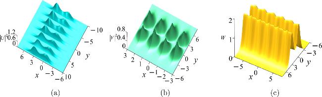
Figure 1. The nondegenerate single soliton with t=0: (a) the multiple double-hump soliton, (b) the double-row multiple taper soliton, (c) the sawtooth double-striped soliton. The parameters are chosen as k1=1 + 0.1i, m1=0.85 + 0.1i, c11=0, and ${c}_{11}^{{\prime} }=0.$ |
In figure 1(a), it can be seen that the short-wave component U exhibits a double-hump structure along the x-direction, while displaying clear pulse-like characteristics in the y-direction. Specifically, within each cycle, the soliton appears in a relatively narrow range. Therefore, considering the behavior of the soliton in both the x- and y-directions, the component U forms multiple double-hump structures. In figure 1(b), the short-wave component V also exhibits a double-hump structure along the x-direction, accompanied by a periodically arranged triangular waveform in the y-direction. This combination produces a double-row, multi-taper structure. Additionally, figure 1(c) shows that the long-wave component W appears as a soliton with a double-striped structure, where each stripe takes on a sawtooth-like waveform along the y-direction.
Changing the values of the wavenumbers k1 and m1 in figure 1(a) results in figure 2.
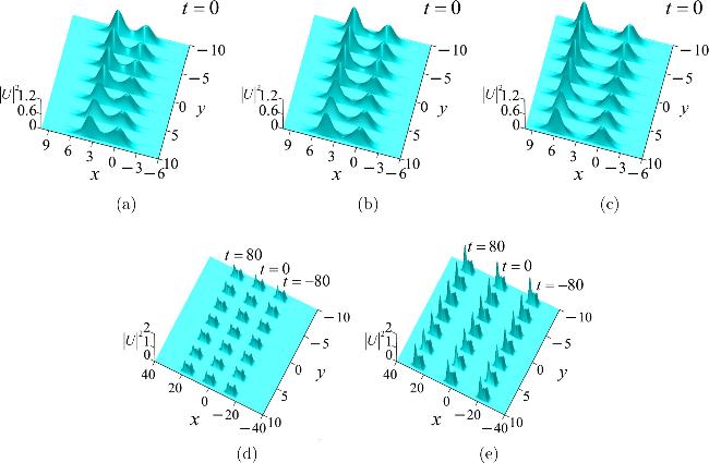
Figure 2. Multiple double-hump single solitons with different wavenumbers. The parameters are chosen as: (a) k1=1+0.1i, m1=0.9+0.1i; (b) k1=1+0.1i, m1=0.95+0.1i; (c) k1=1+0.1i, m1=0.99+0.1i; (d) k1=1+0.1i, m1=0.84+0.1i; (e) k1=1+0.15i, m1=0.84+0.15i. |
By comparing figures 2(a)-(c), it is evident that when the real parts of the wavenumbers k1 and m1 are close to each other, the distance between the two humps of the nondegenerate one-soliton along the x-axis increases. Furthermore, from the time-series plots in figures 2(d) and (e), it can be observed that as the imaginary parts of the wavenumbers increase, the propagation velocity of the nondegenerate single soliton increases. This phenomenon is consistent with the earlier conclusion that the imaginary part of the wavenumber determines the propagation velocity of the nondegenerate one-soliton [9,13,15].
When the functional forms of p1(y) and q1(y) are chosen as described in the caption of figure 3, the resulting M-shaped waveform for the nondegenerate single soliton is illustrated in the figure below
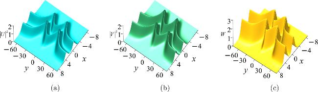
Figure 3. The M-shape nondegenerate single soliton with t=0. The parameter values are k1=1+0.5i, m1=0.95+0.5${\rm{i}},{c}_{11}=0,{c}_{11}^{{\prime} }$=$0,{p}_{1}(y)=22{{\rm{e}}}^{10{\rm{s}}{\rm{e}}{\rm{c}}{\rm{h}}(0.1y+2)}+{{\rm{e}}}^{10{\rm{s}}{\rm{e}}{\rm{c}}{\rm{h}}(0.1y-2)}+{\rm{s}}{\rm{e}}{\rm{c}}{\rm{h}}(0.1y+2)$ $\tanh (0.1y+2)\,\cdot $ ${{\rm{e}}}^{10{\rm{s}}{\rm{e}}{\rm{c}}{\rm{h}}(0.1y+2)}+{\rm{s}}{\rm{e}}{\rm{c}}{\rm{h}}(0.1y-2)\tanh $ ${(0.1y-2){{\rm{e}}}^{10{\rm{s}}{\rm{e}}{\rm{c}}{\rm{h}}(0.1y-2)}]}^{0.5},$ and ${q}_{1}(y)=2\left[7.22\left({{\rm{e}}}^{10{\rm{s}}{\rm{e}}{\rm{c}}{\rm{h}}(0.1y+2)}+{{\rm{e}}}^{10{\rm{s}}{\rm{e}}{\rm{c}}{\rm{h}}(0.1y-2)}\right)\,+\right.$ $3.8\cdot {\rm{s}}{\rm{e}}{\rm{c}}{\rm{h}}(0.1y+2)\tanh (0.1y+2){{\rm{e}}}^{10{\rm{s}}{\rm{e}}{\rm{c}}{\rm{h}}(0.1y+2)}\,+$ ${\left.3.8{\rm{s}}{\rm{e}}{\rm{c}}{\rm{h}}(0.1y-2)\tanh (0.1y-2){{\rm{e}}}^{10{\rm{s}}{\rm{e}}{\rm{c}}{\rm{h}}(0.1y-2)}\right]}^{0.5}.$ |
In figure 3, the nondegenerate single soliton structures of the components U, V and W exhibit similar characteristics. These structures manifest M-shaped double-hump profiles along the x-axis and simultaneously display M-shaped patterns in the x-y plane.
By taking N=2 in equations (14 ) and (15 ), we derive the general nondegenerate double-soliton solution of the system. By choosing ${p}_{1}(y)=\exp \left(-{y}^{2}\right)$, ${p}_{2}(y)=0.8\exp \left(-{y}^{2}\right)$, and q1(y)=q2(y)=sech(y), the waveforms of the short-wave components U and V along the y-direction can be confined to a finite domain.
As shown in figures 4(a)-(d), the two double-peak dromion-like solitons in the component U approach each other and undergo a collision, exhibiting no significant change in their waveforms before and after the interaction. In contrast, as shown in figures 4(e)-(h), the heights of the two double-peak dromion-like solitons in the component V undergo considerable alteration before and after the collision, indicating that the interaction is inelastic. Finally, as illustrated in figures 4(i)-(l), the component W consists of two crosswise-oriented double-stripe solitons, which move toward each other, resulting in a continuous shift of the contact point in the positive direction along the y-axis.
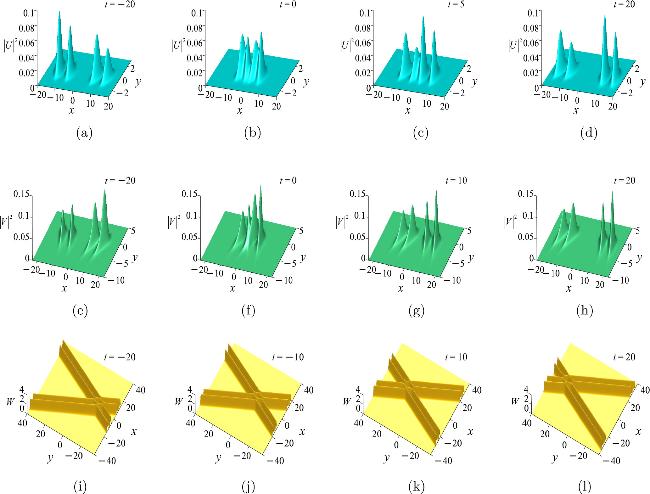
Figure 4. Interaction of nondegenerate double solitons: (a)-(h) dromion-like solitons, (i)-(l) double-stripe solitons. The parameters are chosen as k1=0.99+0.25i, k2=-0.99-0.25i, m1=1+0.25i, m2=-1-0.25i, cjl=2, and ${c}_{jl}^{{\prime} }=2\,(j,l=1,2)$. |
In previous studies, two nondegenerate solitons of the same component typically exhibited similar shapes. In this work, however, by selecting different functional forms for p1(y) and p2(y), as well as for q1(y) and q2(y), we demonstrate that two nondegenerate solitons of the same component can have distinctly different structures. For example, when ${p}_{1}=\exp \left(-{y}^{2}\right)$, ${p}_{2}=\exp \left(y+4\right)$, ${q}_{1}={\rm{{\rm{sech}} }}(-{y}^{2})$, and ${q}_{2}=\exp \left(y+4\right)$, the corresponding graphs of the nondegenerate double solitons for each component are illustrated in figure 5.
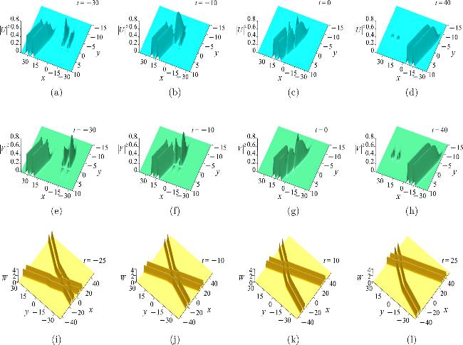
Figure 5. Two nondegenerate solitons of the same component with different structures: (a)-(h) the dromion-like soliton and the solitoff, (i)-(l) the planar kink-type double-stripe soliton and the piecewise linear double-stripe soliton. The parameters are chosen as k1=0.999+0.25i, k2=-0.999- 0.25i, m1=1 + 0.25i, m2=- 1 -0.25i, cjl=2, and ${c}_{jl}^{{\prime} }=2\,(j,l=1,2).$ |
figures 5(a) and (e) illustrate that the structures of the components U and V are relatively similar, both comprising a double-striped solitoff and a double-peaked dromion-like soliton. Further analysis of figures 5(a)-(d) and 5(e)-(h) reveals that in components U and V, the waveforms of the solitoffs and dromion-like solitons change significantly before and after the collision, indicating an inelastic interaction between these two solitons. Additionally, figure 5(i) shows that the component W consists of a planar kink-type double-striped soliton and a piecewise linear double-striped soliton. As seen in figures 5(i)-(l), these two solitons approach each other within the component W, leading to a gradual shift of the contact point in the positive y-axis direction. Furthermore, it is observed that the kink structure of the planar kink double-striped soliton disappears after it comes into contact with the piecewise linear double-striped soliton.
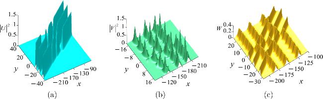
By setting N=3 in equations (14 ) and (15 ), the general nondegenerate three-soliton solution of the system can be derived. Subsequently, choosing ${p}_{j}(y)=\exp (y)$ and ${q}_{l}(y)\,=\sin (0.5y)$ yields the following solitoff-type nondegenerate three-soliton graphs.
figure 6(a) shows that the component U exhibits a structure composed of multiple columns of solitoffs. In figure 6(b), the component V displays three pairs of solitoffs whose waveform heights vary periodically along the y-direction, resulting in numerous peaks. In figure 6(c), the component W consists of six pairs of solitoffs, with three pairs arranged along the y-direction forming wavy patterns. The remaining three pairs of straight solitoffs are arranged diagonally, interacting with the first set to create a mesh-like structure.
Figure 6. Nondegenerate triple solitons of the solitoff-type with t=-60: (a) multiple columns of solitoffs, (b) three pairs of multi-peak solitoffs, (c) the mixture of wavy and straight solitoffs. The parameters are chosen as k1=-0.333+i, k2=-0.333+1.2i, k3=- 0.333+1.4i, m1=-0.32+i, m2=-0.32 + 1.2i, m3=-0.32 + 1.4i, cjl=0, and ${c}_{jl}^{{\prime} }=0\,\,(j,l=1,2,3).$ |
4. Conclusion
In this paper, we derive the general nondegenerate N-soliton solution for the (2+1)-dimensional three-component long-wave-short-wave resonance system using the Hirota bilinear method. By choosing different functional forms for the arbitrary functions involving the variable y in this solution, we construct several novel types of nondegenerate solitons. These include M-shaped, multiple double-hump, and sawtooth double-striped solitons, as well as double dromion-like solitons confined within a finite domain in the y-direction, and solitoff-type three solitons with distinct waveforms.
It is important to note that, we most likely cannot obtain explicit analytic expressions of ajl(y) and bjl(y) from equation (8 ) by choosing different functional forms of pj(y), ${p}_{l}^{* }(y)$, qj(y) and ${q}_{l}^{* }(y)$. For this case, numerical integration methods can be used to compute the values of ajl(y) and bjl(y), enabling the plotting of the waveforms of nondegenerate solitons.
Furthermore, analogous nondegenerate soliton solutions with the characteristic of variable separation may also arise in other coupled systems. For example, in multi-component Mel'nikov coupled systems [42,43], the absence of partial derivatives with respect to t in the short-wave components enables the derivation of general nondegenerate N-soliton solutions in terms of the separated variable t. Consequently, this work offers a novel theoretical framework and research perspective for investigating nondegenerate soliton solutions in other complex coupled systems.
Acknowledgments
This work was supported by the National Natural Science Foundation of China, Grant No. 12375006.
Conflicts of interest
The authors declare that they have no conflicts of interest to report regarding the present study.