


1. Introduction
Research of discrete integrable systems has undergone a great development in recent decades [1], in which one of the central roles is played by the so-called multidimensional consistency (MDC) property [2-4]. Based on this property and other extra conditions, 2D quadrilateral equations and 3D octahedron equations with MDC property were classified by Adler, Bobenko and Suris [5,6]. The MDC property can be viewed as a ‘primitive' discrete integrability, which directly leads to Lax pair and auto Bäcklund transformation (BT) of the lattice equation. The BT can be used to generate soliton solutions. Pedagogical examples can be found in [7-9]. There are also non-auto BTs, which connect solutions of different equations. In some cases, a BT and the two equations compose a consistent triplet [10], which has played a key role in generating polynomial/rational solutions of lattice equations [10,11]. A consistent triplet can also be generated by using addition formulae of trigonometric functions and elliptic functions [12]. This gives a lot of simple trigonometric function solutions to lattice equations. In a recent paper [13], starting from a simple sinusoidal function as a seed, using the BT constructed from the MDC property, a new trigonometric function soliton solution was derived for the lattice modified Korteweg-de Vries (mKdV) equation and a continuous counterpart was obtained for the continuous mKdV equation from continuum limit. These solutions are new and they are not a period degeneration of the known elliptic solitons (cf. [14,15]).
In this paper, we focus on the discrete Schwarzian Korteweg-de Vries (SKdV) equation: 1.1 ), to derive soliton solutions in terms of trigonometric functions. In addition, by taking continuum limits we can get new solutions for the continuous SKdV equation
$\begin{eqnarray}\begin{array}{l}p({v}_{n,m}-{v}_{n,m+1})({v}_{n+1,m}-{v}_{n+1,m+1})\\ \,\,-q({v}_{n,m}-{v}_{n+1,m})({v}_{n,m+1}-{v}_{n+1,m+1})=0,\end{array}\end{eqnarray}$
where vn,m=v(n, m) is a function defined on ${{\mathbb{Z}}}^{2}$, p and q are spacing parameters of the n-direction and m-direction, respectively. This equation is also known as the cross-ratio equation and Q1(0) equation in the Adler-Bobenko-Suris (ABS) list [5]. Its integrability was proved in [16], and it plays an important role (as a discretization of the Cauchy-Riemann condition) in the study of discrete analytic functions [17]. This equation allows several simple trigonometric functions solutions (see (3.1)). We will take them as seed solutions, using the BT of ( $\begin{eqnarray}{u}_{t}={u}_{xxx}-\frac{3}{2}\frac{{u}_{xx}^{2}}{{u}_{x}}.\end{eqnarray}$
This equation was first introduced by Krichever and Novikov in 1980 [18], and later independently by Weiss in 1983 [19]. The SKdV equation has interesting bi-Hamiltonian structures [20]. For more literatures about the SKdV equation, one can refer to [21].The paper is organized as follows. In section 2 , we introduce some notations, recall the MDC property of quadrilateral equations, and explain how an auto BT arises from the MDC property. Then in section 3 , by using BT we derive soliton solutions for the discrete SKdV equation (1.1 ). Continuum limits are investigated in section 4 and solutions for the continuous SKdV equation are obtained. Finally, concluding remarks are given in section 5 .
2. MDC property and BT
In this section, for convenience, we employ conventional notations for shifts of function v(n, m) defined on ${{\mathbb{Z}}}^{2}$:
$\begin{eqnarray*}\begin{array}{l}v=v(n,m),\,\widetilde{v}=v(n+1,m),\,\widehat{v}=v(n,m+1),\\ \widehat{\widetilde{v}}=v(n+1,m+1).\end{array}\end{eqnarray*}$
The MDC property allows a lattice equation (or a system) to be consistently embedded into a higher dimension [2-4]. For a quadrilateral equation 2.2a ), (2.2b ) and (2.2c ), to compute $\widehat{\widetilde{v}},\,\overline{\widetilde{v}},\,\widehat{\overline{v}}$, respectively. The MDC property means that the values of $\overline{\widehat{\widetilde{v}}}$ computed from the three right-hand-side equations in (2.2) are same.
$\begin{eqnarray}Q(v,\widetilde{v},\widehat{v},\widehat{\widetilde{v}};p,q)=0,\end{eqnarray}$
where p, q respectively serve as spacing parameters in n and m directions, we introduce a third dimension l with a corresponding lattice parameter r. The corresponding shift is denoted by $\overline{v}=v(n,m,l+1)$, see figure 1. The MDC property of this case can be geometrically described as a consistency around a cube (CAC): the following six equations, $\begin{eqnarray}\begin{array}{l}Q(v,\widetilde{v},\widehat{v},\widehat{\widetilde{v}};p,q)=0\quad (\,\rm{bottom}\,),\\ Q(\overline{v},\overline{\widetilde{v}},\overline{\widehat{v}},\overline{\widehat{\widetilde{v}}};p,q)=0\quad (\,\rm{top}\,),\end{array}\end{eqnarray}$
$\begin{eqnarray}\begin{array}{l}Q(v,\widetilde{v},\overline{v},\overline{\widetilde{v}};p,r)=0\quad (\,\rm{left}\,),\\ Q(\widehat{v},\widehat{\widetilde{v}},\widehat{\overline{v}},\widehat{\overline{\widetilde{v}}};p,r)=0\quad (\,\rm{right}\,),\end{array}\end{eqnarray}$
$\begin{eqnarray}\begin{array}{c}Q(v,\bar{v},\hat{v},\hat{\bar{v}};r,q)=0\,(\,\rm{back}\,),\\ Q(\tilde{v},\mathop{\hat{v}}\limits^{\unicode{x0007E}},\mathop{\bar{v}}\limits^{\unicode{x0007E}},\mathop{\hat{\bar{v}}}\limits^{\unicode{x0007E}};r,q)=0\,(\,\rm{front}\,),\end{array}\end{eqnarray}$
can consistently appear on the six faces of the cube in figure 1. In practice, for the given initial values $(v,\widetilde{v},\widehat{v},\overline{v})$ (see the black dots in figure 1), we use the left-hand-side equations in (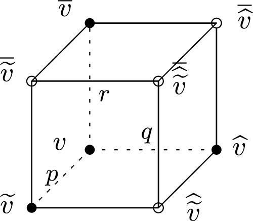
Figure 1. Consistent cube of the quadrilateral equation ( |
Once the equations in (2.2) compose a consistent cube, we write the top equation in the following form 2.1 ), except replacing v by $\overline{v}$. If we consider both v and $\overline{v}$ to be solutions of equation (2.1 ), then, the two side equations, i.e.2.1 ), connecting its solutions v and $\overline{v}$.
$\begin{eqnarray}Q(\overline{v},\widetilde{\overline{v}},\widehat{\overline{v}},\widehat{\widetilde{\overline{v}}};p,q)=0,\end{eqnarray}$
which can be considered to be the same as equation ( $\begin{eqnarray}Q(v,\widetilde{v},\overline{v},\widetilde{\overline{v}};p,r)=0,\end{eqnarray}$
$\begin{eqnarray}Q(v,\bar{v},\hat{v},\hat{\bar{v}};r,q)=0,\end{eqnarray}$
compose an auto BT of equation (Demonstrative examples of using such BTs to find soliton solutions can be found in [7-9]. In addition, rewriting $\overline{v}=g/f$ and introducing $\Psi$=(g, f)T, the BT (2.4) may yield a coupled linear system of $\Psi$, which turns out to be a Lax pair of equation (2.1 ). More examples about constructing Lax pairs under the MDC property can be found in [22].
Next, we introduce a lemma which can be proven through direct calculation.
The relation
$\begin{eqnarray}{{\rm{\Phi }}}_{a}(b){{\rm{\Phi }}}_{c}(d)={{\rm{\Phi }}}_{a+c}(b){{\rm{\Phi }}}_{c}(d-b)+{{\rm{\Phi }}}_{a}(b-d){{\rm{\Phi }}}_{a+c}(d)\end{eqnarray}$
holds, where $\begin{eqnarray}{{\rm{\Phi }}}_{a}(c)=\frac{\sin (a+c)}{\sin (a)\sin (c)}\end{eqnarray}$
and a, b, c are arbitrary numbers.This lemma is useful in deriving one-soliton solution (1SS) of the discrete SKdV equation (1.1 ) using its BT.
3. Trigonometric 1-soliton solution
The discrete SKdV equation (1.1 ) has the following solutions (together with the parameterization of the spacing parameters p and q) [12]:
$\begin{eqnarray}\begin{array}{rcl}v & =& {\rm{\tan }}(\alpha )-n{\rm{\tan }}(a)-m{\rm{\tan }}(b),\,p={{\rm{\tan }}}^{2}(a),\\ q & =& {{\rm{\tan }}}^{2}(b),\end{array}\end{eqnarray}$
$\begin{eqnarray}v={\rm{\tan }}(\alpha ),\,p={\sin }^{2}(a),\quad q={\sin }^{2}(a),\end{eqnarray}$
$\begin{eqnarray}v=\sin (2\alpha )-n\sin (2a)-m\sin (2b),\qquad p={\sin }^{2}(a),\quad q={\sin }^{2}(b),\end{eqnarray}$
where $\begin{eqnarray}\alpha =an+bm+{\alpha }_{0},\end{eqnarray}$
a, b and α0 are arbitrary constants. Next, by means of BT, we will derive soliton solutions from the above seeds.3.1. 1SS from (3.1a)
The discrete SKdV equation (1.1 ) is CAC. Its BT of the form (2.4) reads (with parameterization in (3.1a ))3.1a ), $\overline{v}$ is considered to be a new solution, and c is the BT parameter.
$\begin{eqnarray}{{\rm{\tan }}}^{2}(a)(v-\overline{v})(\widetilde{v}-\widetilde{\overline{v}})-{{\rm{\tan }}}^{2}(c)(v-\widetilde{v})(\overline{v}-\widetilde{\overline{v}})=0,\end{eqnarray}$
$\begin{eqnarray}{{\rm{\tan }}}^{2}(c)(v-\widehat{v})(\overline{v}-\widehat{\overline{v}})-{{\rm{\tan }}}^{2}(b)(v-\overline{v})(\widehat{v}-\widehat{\overline{v}})=0,\end{eqnarray}$
where v is given in (We look for $\overline{v}$ in the following form 3.4 ) into the BT (3.3) yields a coupled system of w:
$\begin{eqnarray}\overline{v}={\rm{\tan }}(\alpha +c)-n{\rm{\tan }}(a)-m{\rm{\tan }}(b)-{\rm{\tan }}(c)+w,\end{eqnarray}$
where w is to be determined. Substituting ( $\begin{eqnarray}\begin{array}{rcl} & & \widetilde{w}\quad =\frac{{\rm{\tan }}(c){\rm{\tan }}(\widetilde{\alpha })\left[{\rm{\tan }}(c){\rm{\tan }}(\alpha )+{\rm{\tan }}(a){\rm{\tan }}(\widetilde{\alpha }+c)\right]w}{{\rm{\tan }}(c){\rm{\tan }}(\alpha )\left[{\rm{\tan }}(c){\rm{\tan }}(\widetilde{\alpha })-{\rm{\tan }}(a){\rm{\tan }}(\alpha +c)\right]-{\rm{\tan }}(a)w},\end{array}\end{eqnarray}$
$\begin{eqnarray}\begin{array}{rcl} & & \widehat{w}\quad =\frac{{\rm{\tan }}(c){\rm{\tan }}(\widehat{\alpha })\left[{\rm{\tan }}(c){\rm{\tan }}(\alpha )+{\rm{\tan }}(b){\rm{\tan }}(\widehat{\alpha }+c)\right]w}{{\rm{\tan }}(c){\rm{\tan }}(\alpha )\left[{\rm{\tan }}(c){\rm{\tan }}(\widehat{\alpha })-{\rm{\tan }}(b){\rm{\tan }}(\alpha +c)\right]-{\rm{\tan }}(b)w}.\end{array}\end{eqnarray}$
To solve out w, we write it as 2.6 ). The system (3.7 ) can be diagonalized as the following 3.8 ) that3.4 ) we obtain a 1SS of the discrete SKdV equation (1.1 ): (here we skip ‘bar')
$\begin{eqnarray}w=\frac{f}{g}\end{eqnarray}$
and introduce $\Psi$=(f, g)T. Then, from (3.13) we have $\begin{eqnarray}\widetilde{{\rm{\Psi }}}=M{\rm{\Psi }},\,\,\widehat{{\rm{\Psi }}}=N{\rm{\Psi }},\end{eqnarray}$
where $\begin{eqnarray*}M=\left(\begin{array}{cc}{{\rm{\Phi }}}_{a}(c)\frac{\cos (\alpha +c)\sin (\widetilde{\alpha })}{\cos (\widetilde{\alpha }+c)\sin (\alpha )} & 0\\ -{\cot }^{2}(c)\cot (\alpha )\cot (\widetilde{\alpha }) & {{\rm{\Phi }}}_{a}(-c)\frac{\cos (\widetilde{\alpha }+c)\sin (\alpha )}{\cos (\alpha +c)\sin (\widetilde{\alpha })}\end{array}\right),\end{eqnarray*}$
$\begin{eqnarray*}N=\left(\begin{array}{cc}{{\rm{\Phi }}}_{b}(c)\frac{\cos (\alpha +c)\sin (\widehat{\alpha })}{\cos (\widehat{\alpha }+c)\sin (\alpha )} & 0\\ -{\cot }^{2}(c)\cot (\alpha )\cot (\widehat{\alpha }) & {{\rm{\Phi }}}_{b}(-c)\frac{\cos (\widehat{\alpha }+c)\sin (\alpha )}{\cos (\alpha +c)\sin (\widehat{\alpha })}\end{array}\right),\end{eqnarray*}$
and Φa(c) is defined as in ( $\begin{eqnarray}\begin{array}{l}\widetilde{R}\widetilde{P}\widetilde{{\rm{\Psi }}}=\left(\begin{array}{cc}{{\rm{\Phi }}}_{a}(c) & 0\\ 0 & {{\rm{\Phi }}}_{a}(-c)\end{array}\right)RP{\rm{\Psi }},\\ \widehat{R}\widehat{P}\widehat{{\rm{\Psi }}}=\left(\begin{array}{cc}{{\rm{\Phi }}}_{b}(c) & 0\\ 0 & {{\rm{\Phi }}}_{b}(-c)\end{array}\right)RP{\rm{\Psi }},\end{array}\end{eqnarray}$
where $\begin{eqnarray}\begin{array}{rcl}P & =& \left(\begin{array}{cc}\frac{\cos (\alpha +c)}{\sin (\alpha )} & 0\\ 0 & \frac{\sin (\alpha )}{\cos (\alpha +c)}\end{array}\right),\\ R & =& \left(\begin{array}{cc}1 & 0\\ \frac{1}{2}\cot (c)\frac{\cos (\alpha -c)}{\cos (\alpha +c)} & 1\end{array}\right).\end{array}\end{eqnarray}$
It then follows from ( $\begin{eqnarray}f={d}_{1}{({{\rm{\Phi }}}_{a}(c))}^{n}{({{\rm{\Phi }}}_{b}(c))}^{m}\sec (\alpha +c)\sin (\alpha ),\end{eqnarray}$
$\begin{eqnarray}\begin{array}{rcl}g & =& {d}_{2}\cos (\alpha +c){({{\rm{\Phi }}}_{a}(-c))}^{n}{({{\rm{\Phi }}}_{b}(-c))}^{m}\csc (\alpha )\\ & & -\frac{1}{2}{d}_{1}\cos (\alpha -c)\cot (c){({{\rm{\Phi }}}_{a}(c))}^{n}{({{\rm{\Phi }}}_{b}(c))}^{m}\csc (\alpha ),\end{array}\end{eqnarray}$
where d1, d2 are constants. Thus we get w=f/g. Then, from ( $\begin{eqnarray}\begin{array}{rcl}v & =& {\sec }^{2}(c){\rm{\tan }}(\alpha )-n{\rm{\tan }}(a)-m{\rm{\tan }}(b)\\ & & -\frac{(1+{\rho }_{n,m}){{\rm{\tan }}}^{2}(\alpha ){\sec }^{2}(c){\rm{\tan }}(c)}{1-{\rho }_{n,m}+(1+{\rho }_{n,m}){\rm{\tan }}(\alpha ){\rm{\tan }}(c)},\end{array}\end{eqnarray}$
where ρn,m is the discrete plane wave factor $\begin{eqnarray}{\rho }_{n,m}={\left(\frac{\sin (c-a)}{\sin (c+a)}\right)}^{n}{\left(\frac{\sin (c-b)}{\sin (c+b)}\right)}^{m}{\rho }_{0,0}\end{eqnarray}$
and ${\rho }_{0,0}=2\frac{{d}_{2}}{{d}_{1}}{\rm{\tan }}(c)$ is a constant.3.2. 1SS from (3.1b)
The calculation is similar to the previous subsection, so we skip some details. The BT of this case reads
$\begin{eqnarray}{\sin }^{2}(a)(v-\overline{v})(\widetilde{v}-\widetilde{\overline{v}})-{\sin }^{2}(c)(v-\widetilde{v})(\overline{v}-\widetilde{\overline{v}})=0,\end{eqnarray}$
$\begin{eqnarray}{\sin }^{2}(c)(v-\widehat{v})(\overline{v}-\widehat{\overline{v}})-{\sin }^{2}(b)(v-\overline{v})(\widehat{v}-\widehat{\overline{v}})=0.\end{eqnarray}$
We assume $\overline{v}$ has the following form 3.1b ) into the above BT yields:
$\begin{eqnarray}\overline{v}={\rm{\tan }}(\alpha +c)+w.\end{eqnarray}$
Substituting it together with ( $\begin{eqnarray}\begin{array}{rcl} & & \widetilde{w}\,=-\frac{\cos (\alpha +c)\sec (\alpha )\sec (\widetilde{\alpha })\sec (\widetilde{\alpha }+c)\sin (c)\sin (a+c)w}{\cos (\widetilde{\alpha }+c)\sec (\alpha )\sec (\widetilde{\alpha })\sec (\alpha +c)\sin (a-c)\sin (c)+\sin (a)w},\end{array}\end{eqnarray}$
$\begin{eqnarray}\begin{array}{rcl} & & \widehat{w}\,=-\frac{\cos (\alpha +c)\sec (\alpha )\sec (\widehat{\alpha })\sec (\widehat{\alpha }+c)\sin (c)\sin (b+c)w}{\cos (\widehat{\alpha }+c)\sec (\alpha )\sec (\widehat{\alpha })\sec (\alpha +c)\sin (b-c)\sin (c)+\sin (b)w}.\end{array}\end{eqnarray}$
Let $w=\frac{f}{g}$ and $\Psi$=(f, g)T, it then follows that 3.16 ) gives rise to a diagonalized system
$\begin{eqnarray}\widetilde{{\rm{\Psi }}}=M{\rm{\Psi }},\,\widehat{{\rm{\Psi }}}=N{\rm{\Psi }},\end{eqnarray}$
where $\begin{eqnarray*}M=\left(\begin{array}{cc}{{\rm{\Phi }}}_{a}(c)\frac{\cos (\alpha +c)}{\cos (\widetilde{\alpha }+c)} & 0\\ -{\csc }^{2}(c)\cos (\widetilde{\alpha })\cos (\alpha ) & {{\rm{\Phi }}}_{a}(-c)\frac{\cos (\widetilde{\alpha }+c)}{\cos (\alpha +c)}\end{array}\right),\end{eqnarray*}$
and $\begin{eqnarray*}N=\left(\begin{array}{cc}{{\rm{\Phi }}}_{b}(c)\frac{\cos (\alpha +c)}{\cos (\widehat{\alpha }+c)} & 0\\ -{\csc }^{2}(c)\cos (\widehat{\alpha })\cos (\alpha ) & {{\rm{\Phi }}}_{b}(-c)\frac{\cos (\widehat{\alpha }+c)}{\cos (\alpha +c)}\end{array}\right).\end{eqnarray*}$
By introducing $\begin{eqnarray}P=\left(\begin{array}{cc}\cos (\alpha +c) & 0\\ 0 & \frac{1}{\cos (\alpha +c)}\end{array}\right),R=\left(\begin{array}{cc}1 & 0\\ \csc (2c)\frac{\cos (\alpha -c)}{\cos (\alpha +c)} & 1\end{array}\right),\end{eqnarray}$
( $\begin{eqnarray}\begin{array}{l}\widetilde{R}\widetilde{P}\widetilde{{\rm{\Psi }}}=\left(\begin{array}{cc}{{\rm{\Phi }}}_{a}(c) & 0\\ 0 & {{\rm{\Phi }}}_{a}(-c)\end{array}\right)RP{\rm{\Psi }},\\ \widehat{R}\widehat{P}\widehat{{\rm{\Psi }}}=\left(\begin{array}{cc}{{\rm{\Phi }}}_{b}(c) & 0\\ 0 & {{\rm{\Phi }}}_{b}(-c)\end{array}\right)RP{\rm{\Psi }},\end{array}\end{eqnarray}$
from which we have $\begin{eqnarray}f={d}_{1}{({{\rm{\Phi }}}_{a}(c))}^{n}{({{\rm{\Phi }}}_{b}(c))}^{m}\sec (\alpha +c),\end{eqnarray}$
$\begin{eqnarray}\begin{array}{l}g={d}_{2}\cos (\alpha +c){({{\rm{\Phi }}}_{a}(-c))}^{n}{({{\rm{\Phi }}}_{b}(-c))}^{m}\\ \,-{d}_{1}\cos (\alpha -c)\cot (c){({{\rm{\Phi }}}_{a}(c))}^{n}{({{\rm{\Phi }}}_{b}(c))}^{m}\csc (2c).\end{array}\end{eqnarray}$
Thus, we obtain w, and then (3.14 ) provide a 1SS of equation (1.1 ) (here we skip ‘bar'): 3.12 ) and here ${\rho }_{0,0}=\frac{{d}_{2}}{{d}_{1}}\sin (2c)$ is a constant.
$\begin{eqnarray}v={\rm{\tan }}(\alpha )-\frac{(1+{\rho }_{n,m}){\rm{\tan }}(c){\sec }^{2}(\alpha )}{1-{\rho }_{n,m}+(1+{\rho }_{n,m}){\rm{\tan }}(\alpha ){\rm{\tan }}(c)},\end{eqnarray}$
where the plane wave factor ρn,m is defined as (3.3. 1SS from (3.1c)
The BT of this case is still (3.13). We assume $\overline{v}$ has the following form 3.1c ) into the BT (3.13) yields a coupled system of w:
$\begin{eqnarray}\overline{v}=\sin (2(\alpha +c))-n\sin (2a)-m\sin (2b)-\sin (2c)+w.\end{eqnarray}$
Substituting it and ( $\begin{eqnarray}\widetilde{w}=\frac{-4\sin (c)\sin (a+c){\sin }^{2}(\widetilde{\alpha })w}{4\sin (a-c)\sin (c){\sin }^{2}(\alpha )-\sin (a)w},\end{eqnarray}$
$\begin{eqnarray}\widehat{w}=\frac{-4\sin (c)\sin (b+c){\sin }^{2}(\widehat{\alpha })w}{4\sin (b-c)\sin (c){\sin }^{2}(\alpha )-\sin (b)w}.\end{eqnarray}$
Again, let $w=\frac{f}{g}$ and $\Psi$=(f, g)T, we are led to a matrix system 3.23 ):
$\begin{eqnarray}\widetilde{{\rm{\Psi }}}=M{\rm{\Psi }},\,\,\widehat{{\rm{\Psi }}}=N{\rm{\Psi }},\end{eqnarray}$
where $\begin{eqnarray*}M=\left(\begin{array}{cc}{{\rm{\Phi }}}_{a}(c)\frac{\sin (\widetilde{\alpha })}{\sin (\alpha )} & 0\\ \frac{1}{4}{\csc }^{2}(c)\csc (\widetilde{\alpha })\csc (\alpha ) & {{\rm{\Phi }}}_{a}(-c)\frac{\sin (\alpha )}{\sin (\widetilde{\alpha })}\end{array}\right),\end{eqnarray*}$
and $\begin{eqnarray*}N=\left(\begin{array}{cc}{{\rm{\Phi }}}_{b}(c)\frac{\sin (\widehat{\alpha })}{\sin (\alpha )} & 0\\ \frac{1}{4}{\csc }^{2}(c)\csc (\widehat{\alpha })\csc (\alpha ) & {{\rm{\Phi }}}_{b}(-c)\frac{\sin (\alpha )}{\sin (\widehat{\alpha })}\end{array}\right).\end{eqnarray*}$
Introducing $\begin{eqnarray}P=\left(\begin{array}{cc}\frac{1}{\sin (\alpha )} & 0\\ 0 & \sin (\alpha )\end{array}\right),R=\left(\begin{array}{cc}1 & 0\\ \frac{-{\csc }^{2}(c)}{8\cot (c)} & 1\end{array}\right),\end{eqnarray}$
we can have a diagonalized version of ( $\begin{eqnarray}\begin{array}{l}\widetilde{R}\widetilde{P}\widetilde{{\rm{\Psi }}}=\left(\begin{array}{cc}{{\rm{\Phi }}}_{a}(c) & 0\\ 0 & {{\rm{\Phi }}}_{a}(-c)\end{array}\right)RP{\rm{\Psi }},\\ \widehat{R}\widehat{P}\widehat{{\rm{\Psi }}}=\left(\begin{array}{cc}{{\rm{\Phi }}}_{b}(c) & 0\\ 0 & {{\rm{\Phi }}}_{b}(-c)\end{array}\right)RP{\rm{\Psi }},\end{array}\end{eqnarray}$
which indicates $\begin{eqnarray}f={d}_{1}{({{\rm{\Phi }}}_{a}(c))}^{n}{({{\rm{\Phi }}}_{b}(c))}^{m}\sin (\alpha ),\end{eqnarray}$
$\begin{eqnarray}\begin{array}{l}g={d}_{2}{({{\rm{\Phi }}}_{a}(-c))}^{n}{({{\rm{\Phi }}}_{b}(-c))}^{m}\csc (\alpha )\\ \,+\frac{1}{8}{d}_{1}{({{\rm{\Phi }}}_{a}(c))}^{n}{({{\rm{\Phi }}}_{b}(c))}^{m}\csc (c)\sec (c)\csc (\alpha ).\end{array}\end{eqnarray}$
Finally, from w=f/g and (3.21 ), we obtain a 1SS of equation (1.1 ) (here we skip ‘bar'): 3.12 ) and here ${\rho }_{0,0}=4\frac{{d}_{2}}{{d}_{1}}\sin (2c)$ is a constant.
$\begin{eqnarray}\begin{array}{l}v=\sin (2\alpha )\cos (2c)-n\sin (2a)-m\sin (2b)\\ \,\,-2{\sin }^{2}(\alpha )\sin (2c)\frac{{\rho }_{n,m}-1}{{\rho }_{n,m}+1},\end{array}\end{eqnarray}$
where the plane wave factor ρn,m is defined as (4. Continuum limits
For the discrete SKdV equation (1.1 ), its continuum limit procedure can be found in [1]. It goes to the continuous SKdV equation (1.2 ). In this section, we implement the same continuum limits on the discrete SKdV equation and its solutions we have derived. As a result, we will obtain trigonometric function solutions of the continuous SKdV equation (1.2 ).
Let us introduce 1.1 ) with parameterization in (3.1a ), i.e. $p={{\rm{\tan }}}^{2}(a),\,q={{\rm{\tan }}}^{2}(b)$, after expanding it into a series of a, we have 3.12 ) yields
$\begin{eqnarray}y=an,\quad V(y,m)=v(n,m),\end{eqnarray}$
which indicates v(n+j, m)=V(y+ja, m). Note that y should be finite, which means n→∞ while a→0. For the discrete SKdV equation ( $\begin{eqnarray*}{\rm{L.H.S.}}(1.1)={a}^{2}[{(V-\widehat{V})}^{2}-{{\rm{\tan }}}^{2}(b){V}_{y}{\widehat{V}}_{y}]+o({a}^{2}),\end{eqnarray*}$
where L.H.S. stands for ‘left-hand-side' and $\widehat{V}=V(y,m+1)$. The leading term gives rise to a semi-discrete SKdV equation $\begin{eqnarray}{(V-\widehat{V})}^{2}-{{\rm{\tan }}}^{2}(b){V}_{y}{\widehat{V}}_{y}=0.\end{eqnarray}$
In this procedure, the plane wave factor ( $\begin{eqnarray}\rho ={\left(\frac{\sin (c-b)}{\sin (c+b)}\right)}^{m}{{\rm{e}}}^{-2\cot (c)y+o(a)}{\rho }_{0,0}.\end{eqnarray}$
The full continuum limit contains two steps. First, one introduces τ=bm and expands (4.2 ) in terms of b. Then, one needs to define 4.4 ) indicates that 4.2 ) in terms of (∂x, ∂t), we are led to an equation in (x, t) from the leading term: 1.2 ) by taking u(x, t)=W(x+t, t/4). In the above procedure, the plane wave factor (4.3 ) yields 3.1a ) and (3.11 ) are 4.7 ).
$\begin{eqnarray}x=y+\tau ,\,\,t=\frac{1}{3}{b}^{2}\tau \end{eqnarray}$
and define V(y, m)=W(x, t). Note that ( $\begin{eqnarray}{\partial }_{y}={\partial }_{x},\,\,{\partial }_{\tau }={\partial }_{x}+\frac{1}{3}{b}^{2}{\partial }_{t}.\end{eqnarray}$
Reorganizing the expansion of ( $\begin{eqnarray}4{W}_{t}={W}_{xxx}+4{W}_{x}-\frac{3}{2}\frac{{W}_{xx}^{2}}{{W}_{x}},\end{eqnarray}$
which is nothing but the continuous SKdV equation ( $\begin{eqnarray}\begin{array}{l}\rho ={{\rm{e}}}^{-2\eta },\,\eta =\cot (c)\,x+\cot (c){\csc }^{2}(c)\,t+{\eta }_{0},\\ {\eta }_{0}\in {\mathbb{C}}.\end{array}\end{eqnarray}$
The counterparts of ( $\begin{eqnarray}W={\rm{\tan }}(x)-x-t\end{eqnarray}$
and $\begin{eqnarray}\begin{array}{l}W={\sec }^{2}(c){\rm{\tan }}(x)-x-t\\ -\frac{(1+{{\rm{e}}}^{-2\eta }){{\rm{\tan }}}^{2}(x){\sec }^{2}(c){\rm{\tan }}(c)}{1-{{\rm{e}}}^{-2\eta }+(1+{{\rm{e}}}^{-2\eta }){\rm{\tan }}(x){\rm{\tan }}(c)},\end{array}\end{eqnarray}$
where η is defined in (For the seed solutions (3.1b ) and (3.1c ), the spacing parameters are $p={\sin }^{2}(a),\,q={\sin }^{2}(b)$. In light of the scheme (4.1 ), we can implement the continuum limit, which gives rise to the following semi-discrete SKdV equation: 1.2 ) by u(x, t)=W(x- t/2, t/4). The counterparts of (3.1b ) and (3.14 ) are 4.7 ).
$\begin{eqnarray}{(V-\widehat{V})}^{2}-{\sin }^{2}(b){V}_{y}{\widehat{V}}_{y}=0.\end{eqnarray}$
The full continuum limit can be implemented by using the same two-step scheme as before. In this case we obtain the continuous SKdV equation $\begin{eqnarray}4{W}_{t}={W}_{xxx}-2{W}_{x}-\frac{3}{2}\frac{{W}_{xx}^{2}}{{W}_{x}},\end{eqnarray}$
which connects the canonical form ( $\begin{eqnarray}W={\rm{\tan }}(x)\end{eqnarray}$
and $\begin{eqnarray}W={\rm{\tan }}(x)-\frac{(1+{{\rm{e}}}^{-2\eta }){\sec }^{2}(x){\rm{\tan }}(c)}{1-{{\rm{e}}}^{-2\eta }+(1+{{\rm{e}}}^{-2\eta }){\rm{\tan }}(x){\rm{\tan }}(c)},\end{eqnarray}$
where η is defined in (For the case related to the seed solution (3.1c ), we get the same semi-discrete SKdV equation (4.10 ) and continuous SKdV equation (4.11 ). The counterparts of (3.1c ) and (3.21 ) are 4.7 ).
$\begin{eqnarray}W=\sin (2x)-2x+4t\end{eqnarray}$
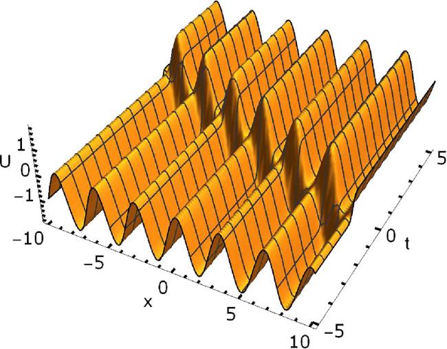
and $\begin{eqnarray}W=\cos (2c)\sin (2x)-2x+4t+2{\sin }^{2}(x)\sin (2c){\rm{\tan }}h(\eta ),\end{eqnarray}$
where η is defined in (We are more interested in the solution (4.15 ) as after removing the linear background -2x+4t, it describes a nonsingular kink solution living on a periodic background. The velocity of the kink is governed by csc2(c). We illustrate such a solution in figure 2.
Figure 2. Shape and motion of U=W+2x-4t where W is given by ( |
Finally, we note that both the continuous SKdV equations (4.6 ) and (4.11 ) are invariant under the transformation 4.9 ), (4.13 ) and (4.15 ), have singularities after being transformed.
$\begin{eqnarray}W(x,t)\to {\rm{i}}W({\rm{i}}x,{\rm{i}}t),\end{eqnarray}$
where i2=-1. For the solutions we presented in this section, this transformation does not change their real-valuedness, but all three solutions, (5. Concluding remarks
The discrete SKdV equation (1.1 ) plays a fundamental role in the study of discrete analytic functions [17]. The SKdV equation (1.2 ) is also quite important. From Wilson's point of view [20], it is considered as a main model to study bi-Hamiltonian structures of other equations in the KdV family (such as the KdV equation and the modified KdV (mKdV) equation). On the other hand, it is well known that both the mKdV equation and the SKdV equation can be formulated by using the eigenfunctions of the Lax pair of the KdV equation [23]. In the discrete case, this fact was described in a recent paper [24], where many equations in the ABS list [5] are formulated by using the eigenfunctions of the Lax pair of the discrete potential KdV equation [24].
In this paper, for the discrete SKdV equation, we have derived soliton solutions from three trigonometric function seeds. The continuum limits of these results yield the counterpart solutions for the continuous SKdV equation. There are many interesting characteristics about these solutions. First, both the discrete and continuous SKdV equations are Möbius transformation invariant. Solutions (3.1b ) and (3.1c ) share same parameterization of lattice parameters, i.e. $p={\sin }^{2}(a)$ and $q={\sin }^{2}(a)$, but they are not connected by any Möbius transformations. In addition, it seems that only (3.1b ) and (4.12 ) can be considered as a ratio of two eigenfunctions of the discrete Schrödinger spectral problem and the continuous Schrödinger spectral problem. So far we do not know how other solutions are related to the eigenfunctions of the discrete and continuous Schrödinger spectral problems. Besides, all the solutions in (3.1) and in (3.11 ), (3.20 ) and (3.27 ) are not the results of period degeneration of elliptic solitons of the discrete SKdV equation (Q1(0) in the ABS list), cf. [14,25]. In other words, they are new solutions with unknown structures.
A recent point of progress is that the trigonometric function multi-soliton solutions of the discrete mKdV equation and continuous mKdV equation were derived using a bilinear method [26]. The bilinear forms are different from those for classical solitons, cf. [7,27]. It also turns out that the multi-soliton solutions (see [26]) contain two types of τ functions: one is a trigonometric function τ function which is the period degeneration of the τ function of elliptic solitons (cf. [15]), the other is a τ function for usual solitons (with special parameterization of soliton numbers). For discrete and continuous SKdV equations, we are also interested in their multi-soliton extension of the solutions obtained in this paper. This will be helpful to understand their structures and to see more insight into these types of solutions that are composed by trigonometric functions.
Acknowledgments
This project is supported by the NSF of China (Grant No. 12271334).