Welcome to visit Communications in Theoretical Physics,
Quantum Physics and Quantum Information

Two imaginarity monotones induced by unified (α, β)-relative entropy

  • Chuanfa Wu ,
  • Zhaoqi Wu
Expand
  • Department of Mathematics, Nanchang University, Nanchang 330031, China

Received date: 2024-12-06

  Revised date: 2025-03-02

  Accepted date: 2025-03-07

  Online published: 2025-05-30

Copyright

© 2025 Institute of Theoretical Physics CAS, Chinese Physical Society and IOP Publishing. All rights, including for text and data mining, AI training, and similar technologies, are reserved.
This article is available under the terms of the IOP-Standard License.

Abstract

Complex numbers play a pivotal role in both mathematics and physics, particularly in quantum mechanics, and are extensively utilized to depict the behavior of microscopic particles. Recognizing the significance of complex numbers, a framework of imaginarity resource theory has recently been established. In this work, we propose two types of imaginarity monotones induced by the unified (α, β)-relative entropy and investigate their properties. Moreover, we give explicit examples to illustrate our results.

Cite this article

Chuanfa Wu , Zhaoqi Wu . Two imaginarity monotones induced by unified (α, β)-relative entropy[J]. Communications in Theoretical Physics, 2025 , 77(9) : 095101 . DOI: 10.1088/1572-9494/adbdbd

1. Introduction

The pivotal and indispensable role of complex numbers in quantum mechanics is undeniable, exerting profound and widespread influence. Complex numbers are important in building the framework of quantum mechanics. By using complex numbers, quantum states and wave functions can accurately describe the behavior of microscopic particles [1-3]. In the dynamic evolution of quantum mechanics [4], complex numbers are particularly crucial. As an integral part of the Schrödinger equation [5-11], the introduction of the imaginary unit 'i' not only accurately depicts the evolutionary track of the wave function over time [12-18], but also endows essential phase information [19-21]. This phase information holds immeasurable value in comprehending unique quantum phenomena like interference [22-24] and diffraction [25-27], while also laying a solid theoretical foundation for the advancement of cutting-edge technologies such as quantum computing [28-30] and quantum communication [31-33]. In terms of experiments, the application of complex numbers in quantum mechanics has been thoroughly validated. By measuring the real and imaginary parts of the wave function [34-42], the accuracy of quantum theory prediction is verified. This further reveals the mysteries of the quantum world. Therefore, we can gain a more comprehensive grasp of the operational laws of the microscopic realm by studying the imaginary numbers.
In light of the pivotal role of complex numbers in quantum mechanics, Hickey and Gour [43] proposed a landmark approach in 2018, treating the imaginary component of quantum states as a resource for investigation and subsequently constructing a comprehensive framework, in which free states and free operations have been elucidated. Many imaginarity quantifiers, such as the trace norm of imaginarity [43], the fidelity of imaginarity [44], the weight of imaginarity [45], the relative entropy of imaginarity [45], the robustness of imaginarity [46], the l1 norm of imaginarity [47], the geometric-like imaginarity [48], have been introduced and studied. The relationship between the relative entropy of imaginarity and the l1 norm of imaginarity and the quantum state order under different quantum channels have been revealed [47].
The above imaginarity measures of a quantum state ρ are defined by taking the minimum over all free states σ for some distance measures between states ρ and σ. It is also possible to define the measures by the distance from a quantum state to its own conjugate, such as the Tsallis relative entropy of imaginarity [49], the α-z Rényi relative entropy imaginarity [50] and the Tsallis relative operator entropy of imaginarity [50]. The problem of imaginarity of Gaussian states [49,51] and Kirkwood-Dirac imaginarity have also been considered [52].
In manipulating the imaginarity resource, the main question is can any two given quantum states be converted into each other via free operations? Sufficient and necessary conditions for the validity of conversion under the circumstance of any two pure states [43] and any two qubit states [46] have been obtained. Moreover, the imaginarity resource in distributed scenarios has been discussed [53]. Like the coherence resource [54,55], the freezing imaginarity of quantum state [56] and the nonlocal advantages of imaginarity [57] have been investigated. The connections between coherence and imaginarity have also been explored [58,59].
The remainder of this paper is arranged as follows. In section 2, we review the fundamental concepts of the quantum imaginary resource theory. In section 3, we propose two imaginarity monotones induced by the unified-(α, β) relative entropy and explore their properties. In section 4, we give some examples to illustrate our results. The conclusion is provided in section 5.

2. Preliminaries

We denote by ${ \mathcal H }$f a d-dimensional Hilbert space, ${\{| j\rangle \}}_{j=0}^{d-1}$ a fixed orthonormal basis in ${ \mathcal H }$, ${ \mathcal D }({ \mathcal H })$ as the set of density operators (quantum states) ρ acting on ${ \mathcal H }$ and ρ* the conjugate of ρ. We recall the framework of the imaginarity resource theory.
Definition 1 [43] Let ρ be a quantum state on ${ \mathcal H }$. ρ is a free state or real state, if
$\begin{eqnarray}\rho =\displaystyle \sum _{jk}{\rho }_{jk}\,| j\rangle \langle k| ,\end{eqnarray}$
where ${\rho }_{jk}\in {\mathbb{R}}$ for arbitrary j,k ∈ {0, 1, …, d-1}. We denote the set of all real states by ${ \mathcal F }$. It can be easily obtained that $\rho \in { \mathcal F }$ if and only if ρ is symmetric, that is, ρT=ρ, where ρT denotes the transpose of ρ.
Definition 2 [43]Let λ be a quantum operation, ρ be a quantum state and ${\rm{\Lambda }}(\rho )={\sum }_{j}\,{K}_{j}\rho {K}_{j}^{\dagger }$. λ is a free operation or real operation if
$\begin{eqnarray}\langle m| {K}_{j}| n\rangle \in {\mathbb{R}},\end{eqnarray}$
for arbitrary j and m, n ∈ {0, 1, …, d-1}.
Definition 3 [43] An imaginarity measure is a functional M: ${ \mathcal D }({ \mathcal H })\to [0,\infty )$ satisfying the following properties:
(M1) Nonnegativity. M(ρ) ≥ 0, M(ρ)=0 if and only if $\rho \in { \mathcal F }$.
(M2) Imaginarity monotonicity. M(λ(ρ)) ≤ M(ρ) whenever λ is a free operation.
(M3) Strong imaginarity monotonicity. M(ρ) ≥ ∑j pj M(ρj), where ${p}_{j}={\rm{tr}}({K}_{j}\rho {K}_{j}^{\dagger })$, ${\rho }_{j}={K}_{j}\rho {K}_{j}^{\dagger }/{p}_{j}$ with free Kraus operators Kj.
(M4) Convexity. ∑j pj M(ρj) ≥ M(∑j pj ρj) for any set of states {ρj} and any pj ≥ 0 with ∑j pj =1.
Besides, the following property (M5) has also been introduced.
(M5) Additivity. M(1 ⊕ (1-p)ρ2)=pM(ρ1)+(1-p)M(ρ2), where p ∈ (0, 1).
It has been proven that (M2) and (M5) are equivalent to (M3) and (M4) [45]. We will call M an imaginarity monotone if it satisfies (M1), (M2) and (M4).
Recently, many imaginarity measures have been proposed. The relative entropy of imaginarity is defined by [45]
$\begin{eqnarray}{M}_{r}(\rho )=S\left[\frac{1}{2}(\rho +{\rho }^{{\rm{T}}})\right]-S(\rho ),\end{eqnarray}$
Tsallis relative entropy of imaginarity is defined by [49]
$\begin{eqnarray}{M}_{T,u}(\rho )=1-{\rm{tr}}\left[{\rho }^{u}{({\rho }^{* })}^{1-u}\right],\end{eqnarray}$
where u ∈ (0, 1) and α-z-Rényi relative entropy of imaginarity is defined by [50]
$\begin{eqnarray}{M}_{\alpha ,z}^{R}(\rho )=1-{f}_{\alpha ,z}(\rho ,{\rho }^{* }),\end{eqnarray}$
where fα,z(ρ, σ)=tr${\left({\sigma }^{\frac{1-\alpha }{2z}}{\rho }^{\frac{\alpha }{z}}{\sigma }^{\frac{1-\alpha }{2z}}\right)}^{z}$ and $0\lt \max \{\alpha ,1-\alpha \}\leqslant z\lt 1$. We denote ${M}_{\alpha ,z}^{R}(\rho )$ by ${M}_{\alpha }^{R}(\rho )$ when α=z.
In addition, there are also many other imaginarity measures, such as the Tsallis relative operator entropy of imaginarity [50], geometric imaginarity measure [46] and so on. They all have elegant properties.
The unified (α, β)-relative entropy has been introduced in [60].
Definition 4 [60] For any α ∈ [0, 1] and any $\beta \in {\mathbb{R}}$, the unified (α, β)-relative entropy is defined by
$\begin{eqnarray}{D}_{\alpha }^{\beta }(\rho | | \sigma )=\left\{\begin{array}{ll}{H}_{\alpha }^{\beta }(\rho | | \sigma ) & \,\rm{if}\,\,0\leqslant \alpha \lt 1,\beta \ne 0,\\ {H}_{\alpha }(\rho | | \sigma ) & \,\rm{if}\,\,0\leqslant \alpha \lt 1,\beta =0,\\ {H}^{\alpha }(\rho | | \sigma ) & \,\rm{if}\,\,0\leqslant \alpha \lt 1,\beta =1,\\ {}_{\frac{1}{\alpha }}H(\rho | | \sigma ) & \,\rm{if}\,\,0\lt \alpha \lt 1,\beta =\frac{1}{\alpha },\\ H(\rho | | \sigma ) & \,\rm{if}\,\alpha =1,\end{array}\right.\end{eqnarray}$
where
$\begin{eqnarray}{H}_{\alpha }^{\beta }(\rho | | \sigma )=\frac{1}{(\alpha -1)\beta }[{({\rm{tr}}({\rho }^{\alpha }{\sigma }^{1-\alpha }))}^{\beta }-1],\end{eqnarray}$
$\begin{eqnarray}{H}_{\alpha }(\rho | | \sigma )=\frac{1}{(\alpha -1)}{\mathrm{log}}_{2}({\rm{tr}}({\rho }^{\alpha }{\sigma }^{1-\alpha })),\end{eqnarray}$
$\begin{eqnarray}{H}^{\alpha }(\rho | | \sigma )=\frac{1}{(\alpha -1)}[{\rm{tr}}({\rho }^{\alpha }{\sigma }^{1-\alpha })-1],\end{eqnarray}$
$\begin{eqnarray}{}_{\alpha }H(\rho | | \sigma )=\frac{1}{(\alpha -1)}[{\left({\rm{tr}}({\rho }^{\frac{1}{\alpha }}{\sigma }^{1-\frac{1}{\alpha }})\right)}^{\alpha }-1],\end{eqnarray}$
$\begin{eqnarray}H(\rho | | \sigma )={\rm{tr}}(\rho {\mathrm{log}}_{2}\rho )-{\rm{tr}}(\rho {\mathrm{log}}_{2}\sigma ).\end{eqnarray}$
It can be easily obtained that ${H}_{\alpha }^{\beta }(\rho | | \sigma )$ reduces to the Rényi relative entropy, Tsallis relative entropy and relative entropy when β →0, β=1 and α →1, respectively.
In order to facilitate the subsequent proofs of the theorems, we present the following lemmas.
Lemma 1. [60] The unified (α, β)-relative entropy satisfies the following properties for any quantum states ρ, σ and any α ∈ (0, 1) and β ∈ (0, 1]:
(i) ${D}_{\alpha }^{\beta }(\rho | | \sigma )\geqslant 0$ and ${D}_{\alpha }^{\beta }(\rho | | \sigma )=0$ if ρ=σ.
(ii) ${D}_{\alpha }^{\beta }({ \mathcal E }(\rho )| | { \mathcal E }(\sigma ))\leqslant {D}_{\alpha }^{\beta }(\rho | | \sigma )$ whenever ${ \mathcal E }$ is a quantum operation.
(iii) ${D}_{\alpha }^{\beta }({\sum }_{j}\,{\lambda }_{j}{\rho }_{j}| | {\sum }_{j}\,{\lambda }_{j}{\sigma }_{j})\leqslant {\sum }_{j}\,{\lambda }_{j}{D}_{\alpha }^{\beta }({\rho }_{j}| | {\sigma }_{j})$.
(iv) For any states ρ and σ on H1H2, ${D}_{\alpha }^{\beta }({\rho }_{1}| | {\sigma }_{1})\leqslant {D}_{\alpha }^{\beta }(\rho | | \sigma )$, where ρ1 and σ1 are the partial traces of ρ and σ on H1, respectively.
(v) ${D}_{\alpha }^{\beta }(\rho | | \sigma )$ is increasing with respect to α ∈ (0, 1) for fixed 0 < β≤1.
(vi) ${D}_{\alpha }^{\beta }(\rho | | \sigma )$ is decreasing with respect to β ∈ (0, 1] for fixed 0 < α < 1.
Lemma 2. [49] For any real operation ${ \mathcal E }$ and any state ρ, it holds that
$\begin{eqnarray}{ \mathcal E }({\rho }^{* })={[{ \mathcal E }(\rho )]}^{* }.\end{eqnarray}$
The following lemma plays an important role in the proof of equation (24) in Example 1, and the proof of it is given in appendix A.
Lemma 3. Let $A\gt \sqrt{{B}^{2}+{C}^{2}}$, B2+C2 > 0, α ∈ (0, 1) and $f(x,\theta )=A[{x}^{1-\alpha }+{(1-x)}^{1-\alpha }]+(B\sin \theta +C\cos \theta )[{(1-x)}^{1-\alpha }\,-{x}^{1-\alpha }],$ where $x\in [0,\frac{1}{2}]$, θ ∈ [0, 2π]. Then f(x, θ) attains its maximum value at $({x}_{0},{\theta }_{0})=\left(\frac{1}{{\left(\frac{A+\sqrt{{B}^{2}+{C}^{2}}}{A-\sqrt{{B}^{2}+{C}^{2}}}\right)}^{\frac{1}{\alpha }}+1},\arcsin \frac{B}{\sqrt{{B}^{2}+{C}^{2}}}\right)$.
Finally, lemma 4 is crucial in proving item (i) of theorem 9, and the proof is given in appendix B.
Lemma 4.Suppose that σρ and στ are the quantum state that reaches the minimum in equation (20) when the input states are ρ and τ, respectively. Then pσρ ⊕ (1-p)στ is a quantum state achieving the minimum in equation (20) when the input state is pρ ⊕ (1-p)τ.

3. Imaginarity monotones based on the unified (α, β)-relative entropy

In this section, we mainly investigate two different imaginarity monotones induced by the unified (α, β)-relative entropy, along with its properties.
Now, we define the first imaginarity quantifier induced by unified (α, β)-relative entropy as
$\begin{eqnarray}{M}_{\alpha ,\beta }^{H}(\rho )=\frac{1}{(\alpha -1)\beta }[{({\rm{tr}}({\rho }^{\alpha }{({\rho }^{* })}^{1-\alpha }))}^{\beta }-1],\end{eqnarray}$
where α ∈ (0, 1), β ∈ (0, 1].

Theorem 1. ${M}_{\alpha ,\beta }^{H}(\rho )$ defined by equation (13) is an imaginarity monotone.

Proof.Due to Lemma 1(i), we know that ${M}_{\alpha ,\beta }^{H}(\rho )\,={D}_{\alpha }^{\beta }(\rho | | {\rho }^{* })\geqslant 0$ and

$\begin{eqnarray}{M}_{\alpha ,\beta }^{H}(\rho )=0\iff \rho ={\rho }^{* }\iff \rho \in { \mathcal F }.\end{eqnarray}$
Thus, ${M}_{\alpha ,\beta }^{H}(\rho )$ satisfies (M1).  

From Lemma 1(ii), we know ${D}_{\alpha }^{\beta }(\rho | | \sigma )$ is nonincreasing under any quantum operation when α ∈ (0, 1) and β ∈ (0, 1]. Let ${ \mathcal E }$ be any real operation. Combining Lemma 1(ii) and lemma 2, we have
$\begin{eqnarray*}\begin{array}{rcl}{M}_{\alpha ,\beta }^{H}({ \mathcal E }(\rho )) & =& \frac{1}{(\alpha -1)\beta }[{({\rm{tr}}({ \mathcal E }{(\rho )}^{\alpha }{({({ \mathcal E }(\rho ))}^{* })}^{1-\alpha }))}^{\beta }-1]\\ & =& \frac{1}{(\alpha -1)\beta }[{({\rm{tr}}({ \mathcal E }{(\rho )}^{\alpha }{({ \mathcal E }({\rho }^{* }))}^{1-\alpha }))}^{\beta }-1]\\ & =& {D}_{\alpha }^{\beta }({ \mathcal E }(\rho )| | { \mathcal E }({\rho }^{* }))\\ & \leqslant & {D}_{\alpha }^{\beta }(\rho | | {\rho }^{* })\\ & =& \frac{1}{(\alpha -1)\beta }[{({\rm{tr}}({\rho }^{\alpha }{({\rho }^{* })}^{1-\alpha }))}^{\beta }-1]\\ & =& {M}_{\alpha ,\beta }^{H}(\rho ),\end{array}\end{eqnarray*}$
which implies that (M2) holds.
Let pn ≥ 0 with ∑npn=1 and ${\rho }_{n}\in { \mathcal D }({ \mathcal H }).$ From Lemma 1(iii), we get
$\begin{eqnarray*}\begin{array}{rcl}{M}_{\alpha ,\beta }^{H}\left(\displaystyle \sum _{n}{p}_{n}{\rho }_{n}\right) & =& {D}_{\alpha }^{\beta }\left(\displaystyle \sum _{n}{p}_{n}{\rho }_{n}| | \displaystyle \sum _{n}{p}_{n}{\rho }_{n}^{* }\right)\\ & \leqslant & \displaystyle \sum _{n}{p}_{n}{D}_{\alpha }^{\beta }({\rho }_{n}| | {\rho }_{n}^{* })\\ & =& {\sum }_{n}{p}_{n}{M}_{\alpha ,\beta }^{H}({\rho }_{n}).\end{array}\end{eqnarray*}$
Hence, (M4) is proved. Therefore, ${M}_{\alpha ,\beta }^{H}(\rho )$ is an imaginarity monotone. This completes the proof.
Furthermore, when ρ=∣ψ⟩⟨ψ∣ is a pure state, we have
$\begin{eqnarray}\displaystyle \begin{array}{rcl}{M}_{\alpha ,\beta }^{H}(\rho ) & =& {M}_{\alpha ,\beta }^{H}(| \psi \rangle \langle \psi | )=\frac{1}{(\alpha -1)\beta }\\ & & \times \,[({\rm{tr}}(| \psi \rangle \langle \psi | {\psi }^{* }\rangle \langle {\psi }^{* }| ){)}^{\beta }-1]\\ & =& \frac{1}{(\alpha -1)\beta }[| \langle \psi | {\psi }^{* }\rangle {| }^{2\beta }-1].\end{array}\end{eqnarray}$
In order to measure super-fidelity and sub-fidelity, a quantum network-based experimental scheme has been designed, in which ∣$\Psi$⟩12 is the program state as a mean value of σz of the measured controlling qubit (see figure 4 in [61]). By setting ∣$\Psi$⟩12=∣0⟩∣0⟩ one gets ${\rm{tr}}({\rho }_{1}{\rho }_{2})$ [61]. Noting that ${\rm{tr}}({\rho }_{1}{\rho }_{2})=| \langle \psi | {\psi }^{* }\rangle {| }^{2}$ when ρ1=∣ψ⟩⟨ψ∣ and ρ2=∣ψ*⟩⟨ψ*∣, it can be seen that the quantity in equation (15), i.e., ${M}_{\alpha ,\beta }^{H}(\rho )$ in the pure state case, can be measured using the scheme proposed in [61].
From equation (13), we can deduce that when β=1, ${M}_{\alpha ,\beta }^{H}(\rho )=\frac{1}{1-\alpha }{M}_{T,u}(\rho )$. Excluding the influence of coefficients, ${M}_{\alpha ,\beta }^{H}(\rho )$ reduces to the imaginarity measure in [49]. In addition, ${M}_{\alpha ,\beta }^{H}(\rho )$ has many elegant properties.

Theorem 2.For any quantum state ρ on ${ \mathcal H }$, and α ∈ (0, 1), β ∈ (0, 1], we have $\frac{1}{1-\alpha }{M}_{1-\alpha ,\beta }^{H}(\rho )=\frac{1}{\alpha }{M}_{\alpha ,\beta }^{H}(\rho ).$

Proof.Note that

$\begin{eqnarray*}\displaystyle \begin{array}{rcl}{M}_{1-\alpha ,\beta }^{H}(\rho ) & =& \frac{1}{-\alpha \beta }[{({\rm{tr}}({\rho }^{1-\alpha }{({\rho }^{* })}^{\alpha }))}^{\beta }-1]\\ & =& \frac{1-\alpha }{\alpha }\cdot \frac{1}{(\alpha -1)\beta }[{({\rm{tr}}({\rho }^{1-\alpha }{({\rho }^{* })}^{\alpha }))}^{\beta }-1]\\ & =& \frac{1-\alpha }{\alpha }{M}_{\alpha ,\beta }^{H}({\rho }^{* })=\frac{1-\alpha }{\alpha }{M}_{\alpha ,\beta }^{H}(\rho ).\end{array}\end{eqnarray*}$
So Theorem 2 holds. This completes the proof.  

Theorem 3.(Superadditivity under direct sum) For any quantum state ρ1, ρ2 on ${ \mathcal H }$, p ∈ [0, 1] and α ∈ (0, 1), β ∈ (0, 1], we have ${M}_{\alpha ,\beta }^{H}(p{\rho }_{1}\oplus (1-p){\rho }_{2})\geqslant p{M}_{\alpha ,\beta }^{H}({\rho }_{1})+(1-p){M}_{\alpha ,\beta }^{H}({\rho }_{2})$.

Proof.Direct calculation shows that

$\begin{eqnarray*}\begin{array}{rcl} & & {M}_{\alpha ,\beta }^{H}(p{\rho }_{1}\displaystyle \oplus (1-p){\rho }_{2})\\ & & \quad =\frac{1}{(\alpha -1)\beta }\\ & & \quad \quad \times [({\rm{tr}}({(p{\rho }_{1}\displaystyle \oplus (1-p){\rho }_{2})}^{\alpha }\\ & & \quad \quad \times {(p{\rho }_{1}^{* }\displaystyle \oplus (1-p){\rho }_{2}^{* })}^{1-\alpha }){)}^{\beta }-1]\\ & & \quad =\frac{1}{(\alpha -1)\beta }[({\rm{tr}}(p{\rho }_{1}^{\alpha }{({\rho }_{1}^{* })}^{1-\alpha }\\ & & \quad \quad \,\displaystyle \oplus (1-p){\rho }_{2}^{\alpha }{({\rho }_{2}^{* })}^{1-\alpha }){)}^{\beta }-1]\\ & & \quad =\frac{1}{(\alpha -1)\beta }[(p{\rm{tr}}({\rho }_{1}^{\alpha }{({\rho }_{1}^{* })}^{1-\alpha })\\ & & \quad \quad +\,(1-p){\rm{tr}}({\rho }_{2}^{\alpha }{({\rho }_{2}^{* })}^{1-\alpha }){)}^{\beta }-1],\end{array}\end{eqnarray*}$
and
$\begin{eqnarray*}\begin{array}{l}p{M}_{\alpha ,\beta }^{H}({\rho }_{1})+(1-p){M}_{\alpha ,\beta }^{H}({\rho }_{2})\\ =\,\frac{1}{(\alpha -1)\beta }[p{({\rm{tr}}({\rho }_{1}^{\alpha }{({\rho }_{1}^{* })}^{1-\alpha }))}^{\beta }-p]\\ \,+\frac{1}{(\alpha -1)\beta }[(1-p){({\rm{tr}}({\rho }_{2}^{\alpha }{({\rho }_{2}^{* })}^{1-\alpha }))}^{\beta }-(1-p)]\\ =\,\frac{1}{(\alpha -1)\beta }[p{({\rm{tr}}({\rho }_{1}^{\alpha }{({\rho }_{1}^{* })}^{1-\alpha }))}^{\beta }\\ \,+(1-p){({\rm{tr}}({\rho }_{2}^{\alpha }{({\rho }_{2}^{* })}^{1-\alpha }))}^{\beta }-1].\end{array}\end{eqnarray*}$

Due to the concavity of f(x)=xβ, we obtain
$\begin{eqnarray*}\begin{array}{l}{(p{\rm{tr}}({\rho }_{1}^{\alpha }{({\rho }_{1}^{* })}^{1-\alpha })+(1-p){\rm{tr}}({\rho }_{2}^{\alpha }{({\rho }_{2}^{* })}^{1-\alpha }))}^{\beta }\\ \geqslant p{({\rm{tr}}({\rho }_{1}^{\alpha }{({\rho }_{1}^{* })}^{1-\alpha }))}^{\beta }+(1-p){({\rm{tr}}({\rho }_{2}^{\alpha }{({\rho }_{2}^{* })}^{1-\alpha }))}^{\beta }.\end{array}\end{eqnarray*}$
Therefore, ${M}_{\alpha ,\beta }^{H}(p{\rho }_{1}\oplus (1-p){\rho }_{2})\geqslant p{M}_{\alpha ,\beta }^{H}({\rho }_{1})+(1-p){M}_{\alpha ,\beta }^{H}({\rho }_{2})$. This completes the proof.
Corollary 1. For α ∈ (0, 1) and β ∈ (0, 1], ${M}_{\alpha ,\beta }^{H}(\rho )$ satisfies the additivity under direct sum if and only if β=1.
Proof. From the proof of Theorem 3, it follows that the equality in equation (3) holds if ${\rm{tr}}({\rho }_{1}^{\alpha }{({\rho }_{1}^{* })}^{1-\alpha })={\rm{tr}}({\rho }_{2}^{\alpha }{({\rho }_{2}^{* })}^{1-\alpha })$ or β=1. However, ${\rm{tr}}({\rho }_{1}^{\alpha }{({\rho }_{1}^{* })}^{1-\alpha })={\rm{tr}}({\rho }_{2}^{\alpha }{({\rho }_{2}^{* })}^{1-\alpha })$ can not be true for any quantum states ρ1 and ρ2. Therefore, the equality in equation (3), and thus the additivity for ${M}_{\alpha ,\beta }^{H}(\rho )$ holds if β=1. This completes the proof.  
Theorem 4.For quantum state ρ on ${{ \mathcal H }}_{1}\otimes {{ \mathcal H }}_{2}$, and α ∈ (0, 1), β ∈ (0, 1], we have ${M}_{\alpha ,\beta }^{H}({\rho }_{1})\leqslant {M}_{\alpha ,\beta }^{H}(\rho )$, where ρ1 is the partial trace of ρ on ${{ \mathcal H }}_{1}$.
Proof. Note that ${\rho }_{1}^{* }$ is the partial trace of ρ* on H1 if ρ1 is the partial trace of ρ on H1. Using Lemma 1(iv), we obtain ${D}_{\alpha }^{\beta }({\rho }_{1}| | {\rho }_{1}^{* })\leqslant {D}_{\alpha }^{\beta }(\rho | | {\rho }^{* })$, that is, ${M}_{\alpha ,\beta }^{H}({\rho }_{1})\leqslant {M}_{\alpha ,\beta }^{H}(\rho )$. This completes the proof.  
Theorem 5. (Subadditivity under tensor product) For any quantum state ρ, τ on ${{ \mathcal H }}_{A}$ and ${{ \mathcal H }}_{B}$, respectively, and α ∈ (0, 1), β ∈ (0, 1], we have
$\begin{eqnarray}{M}_{\alpha ,\beta }^{H}(\rho \otimes \tau )\leqslant {M}_{\alpha ,\beta }^{H}(\rho )+{M}_{\alpha ,\beta }^{H}(\tau ).\end{eqnarray}$
Proof. Note that
$\begin{eqnarray*}\begin{array}{rcl} & & {M}_{\alpha ,\beta }^{H}(\rho \displaystyle \otimes \tau )\\ & & \quad =\frac{1}{(\alpha -1)\beta }[{({\rm{tr}}({(\rho \displaystyle \otimes \tau )}^{\alpha }{({(\rho \displaystyle \otimes \tau )}^{* })}^{1-\alpha }))}^{\beta }-1]\\ & & \quad =\frac{1}{(\alpha -1)\beta }[{({\rm{tr}}({(\rho \displaystyle \otimes \tau )}^{\alpha }{({\rho }^{* }\displaystyle \otimes {\tau }^{* })}^{1-\alpha }))}^{\beta }-1]\\ & & \quad =\frac{1}{(\alpha -1)\beta }[{({\rm{tr}}(({\rho }^{\alpha }\displaystyle \otimes {\tau }^{\alpha })({({\rho }^{* })}^{1-\alpha }\displaystyle \otimes {({\tau }^{* })}^{1-\alpha })))}^{\beta }-1]\\ & & \quad =\frac{1}{(\alpha -1)\beta }[{({\rm{tr}}({\rho }^{\alpha }{({\rho }^{* })}^{1-\alpha }){\rm{tr}}({\tau }^{\alpha }{({\tau }^{* })}^{1-\alpha }))}^{\beta }-1]\\ & & \quad =\frac{1}{(\alpha -1)\beta }[{({\rm{tr}}({\rho }^{\alpha }{({\rho }^{* })}^{1-\alpha }))}^{\beta }-1]\\ & & \quad \quad \times [{({\rm{tr}}({\tau }^{\alpha }{({\tau }^{* })}^{1-\alpha }))}^{\beta }-1]\\ & & \quad \quad +\frac{1}{(\alpha -1)\beta }[{({\rm{tr}}({\rho }^{\alpha }{({\rho }^{* })}^{1-\alpha }))}^{\beta }-1]\\ & & \quad \quad +\frac{1}{(\alpha -1)\beta }[{({\rm{tr}}({\tau }^{\alpha }{({\tau }^{* })}^{1-\alpha }))}^{\beta }-1]\\ & & \quad =(\alpha -1)\beta {M}_{\alpha ,\beta }^{H}(\rho ){M}_{\alpha ,\beta }^{H}(\tau )\\ & & \quad \quad +{M}_{\alpha ,\beta }^{H}(\rho )+{M}_{\alpha ,\beta }^{H}(\tau ).\end{array}\end{eqnarray*}$
Since ${M}_{\alpha ,\beta }^{H}(\rho )$, ${M}_{\alpha ,\beta }^{H}(\tau )\geqslant 0$, and α ∈ (0, 1), β ∈ (0, 1], we obtain ${M}_{\alpha ,\beta }^{H}(\rho \otimes \tau )\leqslant {M}_{\alpha ,\beta }^{H}(\rho )+{M}_{\alpha ,\beta }^{H}(\tau )$. This completes the proof.  
Remark 1. (1) From the proof of Theorem 5, it can be seen that the equality in equation (16) holds if ${M}_{\alpha ,\beta }^{H}(\rho )=0$ or ${M}_{\alpha ,\beta }^{H}(\tau )=0$, i.e., if $\rho \in { \mathcal F }$ or $\tau \in { \mathcal F }$. In this case, equation (16) reduces to ${M}_{\alpha ,\beta }^{H}(\rho \otimes \tau )={M}_{\alpha ,\beta }^{H}(\tau )$ or ${M}_{\alpha ,\beta }^{H}(\rho \otimes \tau )={M}_{\alpha ,\beta }^{H}(\rho )$, which implies ancillary independence of the quantifier to some extent.
(2) It is worth pointing out that equation (16) does not hold for any bipartite quantum state ρab. To see this, consider the bipartite state ρab=(∣00⟩⟨00∣-i∣00⟩⟨11∣ +i∣11⟩⟨00∣+∣11⟩⟨11∣)/2. It follows that ${\rho }^{a}={\rho }^{b}=\frac{I}{2}\in { \mathcal F }$. Then ${M}_{\alpha ,\beta }^{H}({\rho }^{a})={M}_{\alpha ,\beta }^{H}({\rho }^{b})=0$ and ${M}_{\alpha ,\beta }^{H}({\rho }^{ab})\gt 0$, which implies that ${M}_{\alpha ,\beta }^{H}({\rho }^{ab})\gt {M}_{\alpha ,\beta }^{H}({\rho }^{a})+{M}_{\alpha ,\beta }^{H}({\rho }^{b})$.
(3) Note that the subadditivity under tensor product is an important property, and it holds for the Tsallis relative entropy of imaginarity, which has not been mentioned in [49]. In comparison, the property in Theorem 5 has not been discussed for the trace norm of imaginarity, the fidelity of imaginarity, the weight of imaginarity, the robustness of imaginarity, the l1 norm of imaginarity and the geometric-like imaginarity in previous literatures.
Theorem 6. For any α ∈ (0, 1) and β ∈ (0, 1], the imaginarity monotone ${M}_{\alpha ,\beta }^{H}(\rho )$ satisfies the following monotonicity:
(1) ${M}_{{\alpha }_{1},\beta }^{H}(\rho )\leqslant {M}_{{\alpha }_{2},\beta }^{H}(\rho )$ for fixed β when α1α2.
(2) ${M}_{\alpha ,{\beta }_{1}}^{H}(\rho )\geqslant {M}_{\alpha ,{\beta }_{2}}^{H}(\rho )$ for fixed α when β1β2.
Proof. (1) From Lemma 1(v), we have ${D}_{{\alpha }_{1}}^{\beta }(\rho | | \sigma )\leqslant {D}_{{\alpha }_{2}}^{\beta }(\rho | | \sigma )$ when β > 0 and α1α2. Letting σ=ρ*, we have ${M}_{{\alpha }_{1},\beta }^{H}(\rho )\leqslant {M}_{{\alpha }_{2},\beta }^{H}(\rho ).$
(2) From Lemma 1(vi), we have ${D}_{\alpha }^{{\beta }_{1}}(\rho | | \sigma )\geqslant {D}_{\alpha }^{{\beta }_{2}}(\rho | | \sigma )$ when β1β2. Letting σ=ρ*, we have ${M}_{\alpha ,{\beta }_{1}}^{H}(\rho )\geqslant {M}_{\alpha ,{\beta }_{2}}^{H}(\rho ).$ This completes the proof.
Theorem 7. For any quantum state ρ, the order of ${M}_{\alpha ,z}^{R}$, ${M}_{\alpha }^{R}$, ${M}_{\alpha }^{T}$ and ${M}_{\alpha ,\beta }^{H}$ is as follows:
$\begin{eqnarray}{M}_{\alpha }^{R}(\rho )\leqslant {M}_{\alpha ,z}^{R}(\rho )\leqslant {M}_{\alpha }^{T}(\rho )\leqslant {M}_{\alpha ,\beta }^{H}(\rho ).\end{eqnarray}$
Proof. From [50], we know that
$\begin{eqnarray}{M}_{\alpha }^{R}(\rho )\leqslant {M}_{\alpha ,z}^{R}(\rho )\leqslant {M}_{\alpha }^{T}(\rho ).\end{eqnarray}$
Using Theorem 6(2), we have
$\begin{eqnarray}{M}_{\alpha }^{T}(\rho )={M}_{\alpha ,1}^{H}(\rho )\leqslant {M}_{\alpha ,\beta }^{H}(\rho ).\end{eqnarray}$
From equations (18-19), we obtain equation (17). This completes the proof.  
In quantum coherence theory [62-65], a common approach for constructing a coherence quantifier for a quantum state ρ is to minimize a distance measure D (ρ, σ) over all incoherent states σ. A similar scheme can be used in quantum imaginary resource theory. Now, we define the second imaginarity monotone induced by unified (α, β)-relative entropy as
$\begin{eqnarray}{M}_{\alpha ,\beta }^{E}(\rho )=\mathop{\min }\limits_{\sigma \in { \mathcal F }}\frac{1}{(\alpha -1)\beta }[{({\rm{tr}}({\rho }^{\alpha }{\sigma }^{1-\alpha }))}^{\beta }-1],\end{eqnarray}$
where α ∈ (0, 1) and β ∈ (0, 1].
Theorem 8. ${M}_{\alpha ,\beta }^{E}(\rho )$ defined by equation (20) is an imaginarity monotone.
Proof. From Lemma 1(i), we can easily obtain that ${M}_{\alpha ,\beta }^{E}(\rho )$ satisfies (M1). For (M2), it follows from Lemma 1(ii) that
$\begin{eqnarray*}{D}_{\alpha }^{\beta }({ \mathcal E }(\rho )| | { \mathcal E }(\sigma ))\leqslant {D}_{\alpha }^{\beta }(\rho | | \sigma ),\end{eqnarray*}$
holds for any real operation ${ \mathcal E }$, which yields that
$\begin{eqnarray*}\mathop{\min }\limits_{\sigma \in { \mathcal F }}{D}_{\alpha }^{\beta }({ \mathcal E }(\rho )| | { \mathcal E }(\sigma ))\leqslant \mathop{\min }\limits_{\sigma \in { \mathcal F }}{D}_{\alpha }^{\beta }(\rho | | \sigma ),\end{eqnarray*}$
Therefore, we have
$\begin{eqnarray*}\begin{array}{rcl}{M}_{\alpha ,\beta }^{E}({ \mathcal E }(\rho )) & =& \mathop{\min }\limits_{\sigma \in { \mathcal F }}\frac{1}{(\alpha -1)\beta }[{({\rm{tr}}({ \mathcal E }{(\rho )}^{\alpha }{\sigma }^{1-\alpha }))}^{\beta }-1]\\ & \leqslant & \mathop{\min }\limits_{\sigma \in { \mathcal F }}\frac{1}{(\alpha -1)\beta }[{({\rm{tr}}({ \mathcal E }{(\rho )}^{\alpha }{({ \mathcal E }(\sigma ))}^{1-\alpha }))}^{\beta }-1]\\ & =& \mathop{\min }\limits_{\sigma \in { \mathcal F }}{D}_{\alpha }^{\beta }({ \mathcal E }(\rho )| | { \mathcal E }(\sigma ))\\ & \leqslant & \mathop{\min }\limits_{\sigma \in { \mathcal F }}{D}_{\alpha }^{\beta }(\rho | | \sigma )\\ & =& \mathop{\min }\limits_{\sigma \in { \mathcal F }}\frac{1}{(\alpha -1)\beta }[{({\rm{tr}}({\rho }^{\alpha }{\sigma }^{1-\alpha }))}^{\beta }-1]\\ & =& {M}_{\alpha ,\beta }^{E}(\rho ).\end{array}\end{eqnarray*}$
Let pn ≥ 0, ∑npn=1 and ${\rho }_{n}\in { \mathcal D }({ \mathcal H }).$ Then we have
$\begin{eqnarray*}\begin{array}{rcl}{M}_{\alpha ,\beta }^{E}\left({\sum }_{n}{p}_{n}{\rho }_{n}\right) & =& \mathop{\min }\limits_{\sigma \in { \mathcal F }}{D}_{\alpha }^{\beta }\left({\sum }_{n}{p}_{n}{\rho }_{n}| | \sigma \right)\\ & \leqslant & {D}_{\alpha }^{\beta }\left({\sum }_{n}{p}_{n}{\rho }_{n}| | {\sum }_{n}{p}_{n}{\sigma }_{n}\right)\\ & \leqslant & {\sum }_{n}{p}_{n}{D}_{\alpha }^{\beta }({\rho }_{n}| | {\sigma }_{n})\\ & =& {\sum }_{n}{p}_{n}{M}_{\alpha ,\beta }^{E}({\rho }_{n}),\end{array}\end{eqnarray*}$
where ${M}_{\alpha ,\beta }^{E}({\rho }_{n})={D}_{\alpha }^{\beta }({\rho }_{n}| | {\sigma }_{n})$. This implies (M4) holds for ${M}_{\alpha ,\beta }^{E}(\rho )$. This completes the proof.
From Theorem 8, we can derive that when α →1, ${M}_{\alpha ,\beta }^{E}(\rho )={M}_{r}(\rho )$ and Theorem 2 degrades to the imaginarity measure induced by relative entropy in [45]. In addition, ${M}_{\alpha ,\beta }^{E}(\rho )$ also has many properties similar to ${M}_{\alpha ,\beta }^{H}(\rho )$.
Theorem 9. For any α ∈ (0, 1) and β ∈ (0, 1], ${M}_{\alpha ,\beta }^{E}(\rho )$ satisfies the following properties:
(1) (Superadditivity under direct sum) For any quantum state ρ1, ρ2 on ${ \mathcal H }$ and p ∈ [0, 1], we have${M}_{\alpha ,\beta }^{E}(p{\rho }_{1}\oplus (1-p){\rho }_{2})\geqslant p{M}_{\alpha ,\beta }^{E}({\rho }_{1})+(1-p){M}_{\alpha ,\beta }^{E}({\rho }_{2})$.
(2) ${M}_{\alpha ,\beta }^{E}(\rho )$ satisfies the additivity under direct sum if and only if β=1.
(3) For quantum state ρ on ${{ \mathcal H }}_{1}\otimes {{ \mathcal H }}_{2}$, we have ${M}_{\alpha ,\beta }^{E}({\rho }_{1})\leqslant {M}_{\alpha ,\beta }^{E}(\rho )$, where ρ1 is the partial trace of ρ on ${{ \mathcal H }}_{1}$.
(4) (Subadditivity under tensor product) For any quantum state ρ, τ on ${{ \mathcal H }}_{A}$ and ${{ \mathcal H }}_{B}$, respectively, we have${M}_{\alpha ,\beta }^{E}(\rho \otimes \tau )\leqslant {M}_{\alpha ,\beta }^{E}(\rho )+{M}_{\alpha ,\beta }^{E}(\tau )$.
(5) ${M}_{\alpha ,{\beta }_{1}}^{E}(\rho )\geqslant {M}_{\alpha ,{\beta }_{2}}^{E}(\rho )$ for fixed α when β1β2.
Proof. (1) Suppose that σ1 and σ2 are the quantum state that reaches the minimum in equation (20) when the input states are ρ1 and ρ2, respectively. Utilizing Lemma 4, we obtain
$\begin{eqnarray*}\begin{array}{l}p{M}_{\alpha ,\beta }^{E}({\rho }_{1})+(1-p){M}_{\alpha ,\beta }^{E}({\rho }_{2})\\ =\,\frac{1}{(\alpha -1)\beta }[p{({\rm{tr}}({\rho }_{1}^{\alpha }{({\sigma }_{1})}^{1-\alpha }))}^{\beta }\\ +\,(1-p){({\rm{tr}}({\rho }_{2}^{\alpha }{({\sigma }_{2})}^{1-\alpha }))}^{\beta }-1]\\ \leqslant \,\frac{1}{(\alpha -1)\beta }[(p{\rm{tr}}({\rho }_{1}^{\alpha }{({\sigma }_{1})}^{1-\alpha })\\ +\,(1-p){\rm{tr}}({\rho }_{2}^{\alpha }{({\sigma }_{2})}^{1-\alpha }){)}^{\beta }-1]\\ =\,\,\frac{1}{(\alpha -1)\beta }[({\rm{tr}}({(p{\rho }_{1}\displaystyle \oplus (1-p){\rho }_{2})}^{\alpha }\\ {(p{\sigma }_{1}\displaystyle \oplus (1-p){\sigma }_{2})}^{1-\alpha }){)}^{\beta }-1]\\ =\,{M}_{\alpha ,\beta }^{E}(p{\rho }_{1}\displaystyle \oplus (1-p){\rho }_{2}),\end{array}\end{eqnarray*}$
where the inequality is true because f(x)=xβ is a convex function. So item (1) holds.  
(2) Imitating the proof of corollary 1, item (2) can be easily obtained, and so we omit it here.
(3) Let $\tilde{\sigma }$ be a quantum state achieving the minimum in equation (20), ${\tilde{\sigma }}_{1}$ be the partial trace of $\tilde{\sigma }$ on ${{ \mathcal H }}_{1}$ and σ1 be any real state on ${{ \mathcal H }}_{1}$. Using Lemma 1(iv), we obtain
$\begin{eqnarray*}\begin{array}{rcl}{M}_{\alpha ,\beta }^{E}(\rho ) & =& \mathop{\min }\limits_{\sigma \in { \mathcal F }}\frac{1}{(\alpha -1)\beta }[{({\rm{tr}}({\rho }^{\alpha }{\sigma }^{1-\alpha }))}^{\beta }-1]\\ & =& \frac{1}{(\alpha -1)\beta }[{({\rm{tr}}({\rho }^{\alpha }{\tilde{\sigma }}^{1-\alpha }))}^{\beta }-1]\\ & =& D(\rho | | \tilde{\sigma })\\ & \geqslant & D({\rho }_{1}| | {\tilde{\sigma }}_{1})\\ & =& \frac{1}{(\alpha -1)\beta }[{({\rm{tr}}({\rho }_{1}^{\alpha }{\tilde{\sigma }}_{1}^{1-\alpha }))}^{\beta }-1]\\ & \geqslant & \mathop{\min }\limits_{{\sigma }_{1}\in { \mathcal F }}\frac{1}{(\alpha -1)\beta }[{({\rm{tr}}({\rho }_{1}^{\alpha }{\sigma }_{1}^{1-\alpha }))}^{\beta }-1]\\ & =& {M}_{\alpha ,\beta }^{E}({\rho }_{1}),\end{array}\end{eqnarray*}$
that is, ${M}_{\alpha ,\beta }^{E}({\rho }_{1})\leqslant {M}_{\alpha ,\beta }^{E}(\rho )$. Hence, item (3) is true.
(4) Suppose that σρ and στ are the quantum state that reaches the minimum value in equation (20) when the input states are ρ and τ, respectively. Then we obtain
$\begin{eqnarray*}\begin{array}{rcl} & & {M}_{\alpha ,\beta }^{E}(\rho \displaystyle \otimes \tau )\\ & & \quad =\mathop{\min }\limits_{\sigma \in { \mathcal F }}\frac{1}{(\alpha -1)\beta }\\ & & \quad \quad \times [{({\rm{tr}}({(\rho \displaystyle \otimes \tau )}^{\alpha }{\sigma }^{1-\alpha }))}^{\beta }-1]\\ & & \quad \leqslant \mathop{\min }\limits_{{\sigma }_{a},{\sigma }_{b}\in { \mathcal F }}\frac{1}{(\alpha -1)\beta }\\ & & \,\times \,[{({\rm{tr}}({(\rho \displaystyle \otimes \tau )}^{\alpha }{({\sigma }_{a}\displaystyle \otimes {\sigma }_{b})}^{1-\alpha }))}^{\beta }-1]\\ & & \quad \leqslant \frac{1}{(\alpha -1)\beta }[{({\rm{tr}}({(\rho \displaystyle \otimes \tau )}^{\alpha }{({\sigma }_{\rho }\displaystyle \otimes {\sigma }_{\tau })}^{1-\alpha }))}^{\beta }-1]\\ & & \quad =\frac{1}{(\alpha -1)\beta }[{({\rm{tr}}(({\rho }^{\alpha }\displaystyle \otimes {\tau }^{\alpha })({\sigma }_{\rho }^{1-\alpha }\displaystyle \otimes {\sigma }_{\tau }^{1-\alpha })))}^{\beta }-1]\\ & & \quad =\frac{1}{(\alpha -1)\beta }[{({\rm{tr}}({\rho }^{\alpha }{\sigma }_{\rho }^{1-\alpha }){\rm{tr}}({\tau }^{\alpha }{\sigma }_{\tau }^{1-\alpha }))}^{\beta }-1]\\ & & \quad =\frac{1}{(\alpha -1)\beta }[{({\rm{tr}}({\rho }^{\alpha }{\sigma }_{\rho }^{1-\alpha }))}^{\beta }-1][{({\rm{tr}}({\tau }^{\alpha }{\sigma }_{\tau }^{1-\alpha }))}^{\beta }-1]\\ & & \quad \quad +\,\frac{1}{(\alpha -1)\beta }[{({\rm{tr}}({\rho }^{\alpha }{\sigma }_{\rho }^{1-\alpha }))}^{\beta }-1]\\ & & \quad \quad +\,\frac{1}{(\alpha -1)\beta }[{({\rm{tr}}({\tau }^{\alpha }{\sigma }_{\tau }^{1-\alpha }))}^{\beta }-1]\\ & & \quad =(\alpha -1)\beta {M}_{\alpha ,\beta }^{E}(\rho ){M}_{\alpha ,\beta }^{E}(\tau )+{M}_{\alpha ,\beta }^{E}(\rho )+{M}_{\alpha ,\beta }^{E}(\tau ).\end{array}\end{eqnarray*}$
Since ${M}_{\alpha ,\beta }^{E}(\rho )$, ${M}_{\alpha ,\beta }^{E}(\tau )\geqslant 0$, and α ∈ (0, 1), β ∈ (0, 1], we obtain ${M}_{\alpha ,\beta }^{E}(\rho \otimes \tau )\leqslant {M}_{\alpha ,\beta }^{E}(\rho )+{M}_{\alpha ,\beta }^{E}(\tau )$, which implies that item (4) holds.
(5) Suppose that $\hat{\sigma }$ is a quantum state reaching the minimum value in the definition of ${M}_{\alpha ,{\beta }_{1}}^{E}(\rho )$, that is,
$\begin{eqnarray*}{M}_{\alpha ,{\beta }_{1}}^{E}(\rho )=\frac{1}{(\alpha -1){\beta }_{1}}[{({\rm{tr}}({\rho }^{\alpha }{\hat{\sigma }}^{1-\alpha }))}^{{\beta }_{1}}-1].\end{eqnarray*}$
Then it is obvious that
$\begin{eqnarray*}{M}_{\alpha ,{\beta }_{2}}^{E}(\rho )=\frac{1}{(\alpha -1){\beta }_{2}}[{({\rm{tr}}({\rho }^{\alpha }{\hat{\sigma }}^{1-\alpha }))}^{{\beta }_{2}}-1].\end{eqnarray*}$
Using Lemma 1(vi), we have
$\begin{eqnarray*}{M}_{\alpha ,{\beta }_{1}}^{E}(\rho )={D}_{\alpha }^{{\beta }_{1}}(\rho \parallel \hat{\sigma })\geqslant {D}_{\alpha }^{{\beta }_{2}}(\rho \parallel \hat{\sigma })={M}_{\alpha ,{\beta }_{2}}^{E}(\rho ).\end{eqnarray*}$
Therefore, item (5) is derived. This completes the proof.
Remark 2. It bears noting that ${M}_{{\alpha }_{1},\beta }^{E}(\rho )\leqslant {M}_{{\alpha }_{2},\beta }^{E}(\rho )$ for fixed β when α1α2 is not true, since when α varies, the quantum state σ that minimizes the quantity in equation (20) may also change accordingly, making it impossible to compare the values of ${M}_{{\alpha }_{1},\beta }^{E}(\rho )$ and ${M}_{{\alpha }_{2},\beta }^{E}(\rho )$.

4. Examples

In this section, we investigate the imaginarity monotones ${M}_{\alpha ,\beta }^{H}(\rho )$ and ${M}_{\alpha ,\beta }^{E}(\rho )$ under some special quantum states.
Example 1. Consider a qubit state ρ expressed in Bloch representation as
$\begin{eqnarray}\rho =\frac{1}{2}({I}+\overrightarrow{r}\cdot \overrightarrow{\sigma })=\frac{1}{2}\left(\begin{array}{cc}1+{r}_{3} & {r}_{1}-{\rm{i}}{r}_{2}\\ {r}_{1}+{\rm{i}}{r}_{2} & 1-{r}_{3}\end{array}\right),\end{eqnarray}$
where $\overrightarrow{r}=({r}_{1},{r}_{2},{r}_{3})$ is a real vector with $r=| \overrightarrow{r}| =\sqrt{{r}_{1}^{2}+{r}_{2}^{2}+{r}_{3}^{2}}\leqslant 1$ and $\overrightarrow{\sigma }=({\sigma }_{x},{\sigma }_{y},{\sigma }_{z})$ with ${\sigma }_{x}=\left(\begin{array}{cc}0 & 1\\ 1 & 0\end{array}\right)$, ${\sigma }_{y}=\left(\begin{array}{cc}0 & -{\rm{i}}\\ {\rm{i}} & 0\end{array}\right)$and ${\sigma }_{z}=\left(\begin{array}{cc}1 & 0\\ 0 & -1\end{array}\right)$. If $\rho \in { \mathcal F }$, we obtain ${M}_{\alpha ,\beta }^{H}(\rho )=0$. Otherwise, it follows from [49], we know that
$\begin{eqnarray}\displaystyle \begin{array}{rcl}{\rm{tr}}[{\rho }^{\alpha }{({\rho }^{* })}^{1-\alpha }] & =& \frac{1}{2{r}^{2}}\left\{(1-r)\left[{\left(r-\frac{{r}_{2}^{2}}{r-{r}_{3}}\right)}^{2}+\frac{{r}_{1}^{2}{r}_{2}^{2}}{{(r-{r}_{3})}^{2}}\right]\right.\\ & & +(1+r)\left[{\left(r-\frac{{r}_{2}^{2}}{r+{r}_{3}}\right)}^{2}\right.+\left.\frac{{r}_{1}^{2}{r}_{2}^{2}}{{(r+{r}_{3})}^{2}}\right]\\ & & \left.+{r}_{2}^{2}[{(1-r)}^{\alpha }{(1+r)}^{1-\alpha }+{(1-r)}^{1-\alpha }{(1+r)}^{\alpha }]\Space{0ex}{4.25ex}{0ex}\right\}.\end{array}\end{eqnarray}$
Therefore, by equation (13), we have
$\begin{eqnarray}\displaystyle \begin{array}{l}{M}_{\alpha ,\beta }^{H}(\rho )=\frac{1}{(\alpha -1)\beta }\left\{\frac{1}{{2}^{\beta }{r}^{2\beta }}\left\{(1-r)\right.\right.\\ \quad \times \,\left[{\left(r-\frac{{r}_{2}^{2}}{r-{r}_{3}}\right)}^{2}+\frac{{r}_{1}^{2}{r}_{2}^{2}}{{(r-{r}_{3})}^{2}}\right]\\ \quad +\,(1+r)\left[{\left(r-\frac{{r}_{2}^{2}}{r+{r}_{3}}\right)}^{2}\right.\\ \quad \left.+\,\frac{{r}_{1}^{2}{r}_{2}^{2}}{{(r+{r}_{3})}^{2}}\right]\\ \quad +\,{r}_{2}^{2}[{(1-r)}^{\alpha }{(1+r)}^{1-\alpha }+{(1-r)}^{1-\alpha }\\ \quad \left.{\left.\times \,{(1+r)}^{\alpha }]\right\}}^{\beta }-1\right\},\end{array}\end{eqnarray}$
for all α ∈ (0, 1) and β ∈ (0, 1], and by equation (20), ${M}_{\alpha ,\beta }^{E}(\rho )$ reads
$\begin{eqnarray}\begin{array}{l}{M}_{\alpha ,\beta }^{E}(\rho )=\frac{1}{(\alpha -1)\beta }\\ \left\{\frac{1}{{2}^{\beta }}\left[{\left(1-\frac{1}{{\left(\frac{(r-\sqrt{{r}_{1}^{2}+{r}_{3}^{2}}){(1-r)}^{\alpha }+(r+\sqrt{{r}_{1}^{2}+{r}_{3}^{2}}){(1+r)}^{\alpha }}{(r+\sqrt{{r}_{1}^{2}+{r}_{3}^{2}}){(1-r)}^{\alpha }+(r-\sqrt{{r}_{1}^{2}+{r}_{3}^{2}}){(1+r)}^{\alpha }}\right)}^{\frac{1}{\alpha }}+1}\right)}^{1-\alpha }\right.\right.\\ \times \left(\left(1-\frac{\sqrt{{r}_{1}^{2}+{r}_{3}^{2}}}{r}\right){\left(\frac{1-r}{2}\right)}^{\alpha }\right.\\ \quad +\left.\left(1+\frac{\sqrt{{r}_{1}^{2}+{r}_{3}^{2}}}{r}\right){\left(\frac{1+r}{2}\right)}^{\alpha }\right)\\ \left.+\left(\left(1+\frac{\sqrt{{r}_{1}^{2}+{r}_{3}^{2}}}{r}\right){\left(\frac{1-r}{2}\right)}^{\alpha }\right.\quad +\left(1-\frac{\sqrt{{r}_{1}^{2}+{r}_{3}^{2}}}{r}\right){\left(\frac{1+r}{2}\right)}^{\alpha }\right)\\ \left.{\left.\times {\left(\frac{1}{{\left(\frac{(r-\sqrt{{r}_{1}^{2}+{r}_{3}^{2}}){(1-r)}^{\alpha }+(r+\sqrt{{r}_{1}^{2}+{r}_{3}^{2}}){(1+r)}^{\alpha }}{(r+\sqrt{{r}_{1}^{2}+{r}_{3}^{2}}){(1-r)}^{\alpha }+(r-\sqrt{{r}_{1}^{2}+{r}_{3}^{2}}){(1+r)}^{\alpha }}\right)}^{\frac{1}{\alpha }}+1}\right)}^{1-\alpha }\right]}^{\beta }-1\right\},\end{array}\end{eqnarray}$
for all α ∈ (0, 1) and β ∈ (0, 1].
The proof of equation (24) is given in appendix C, and the surfaces of ${M}_{\alpha ,\beta }^{H}(\rho )$ and ${M}_{\alpha ,\beta }^{E}(\rho )$ in Equations (23) and (24) are plotted in figure 1.
Figure 1. The variations of ${M}_{\alpha ,\beta }^{H}(\rho )$ and ${M}_{\alpha ,\beta }^{E}(\rho )$ in equation (23) and equation (24) for fixed $\overrightarrow{r}$. Red (blue) surface represents the value of ${M}_{\alpha ,\beta }^{H}(\rho )$ (${M}_{\alpha ,\beta }^{E}(\rho )$). (a)$\overrightarrow{r}=(0,1,0)$ (ρ is a pure state); (b)$\overrightarrow{r}=(\frac{1}{2},\frac{1}{4},\frac{1}{2})$ (ρ is a mixed state).

Remark 3. From appendix C, it can be seen that equation (20) achieves its minimum value when

$\begin{eqnarray*}\sigma =\bar{\sigma }=\frac{1}{2}\left(\begin{array}{cc}1 & 0\\ 0 & 1\end{array}\right),\end{eqnarray*}$
for any state
$\begin{eqnarray*}\tilde{\rho }=\frac{1}{2}\left(\begin{array}{cc}1 & -{r}_{2}{\rm{i}}\\ {r}_{2}{\rm{i}} & 1\end{array}\right),\end{eqnarray*}$
and
$\begin{eqnarray*}{\rm{tr}}({\tilde{\rho }}^{\alpha }{\bar{\sigma }}^{1-\alpha })=\frac{1}{2}\left[{(1-{r}_{2})}^{\alpha }+{(1+{r}_{2})}^{\alpha }\right].\end{eqnarray*}$
By equation (22), we have
$\begin{eqnarray*}\begin{array}{rcl}{\rm{tr}}({\tilde{\rho }}^{\alpha }{({\tilde{\rho }}^{* })}^{1-\alpha }) & =& \frac{1}{2}\left[{(1+{r}_{2})}^{1-\alpha }{(1-{r}_{2})}^{\alpha }\right.\\ & & \left.+{(1+{r}_{2})}^{\alpha }{(1-{r}_{2})}^{1-\alpha }\right].\end{array}\end{eqnarray*}$
Let
$\begin{eqnarray*}\begin{array}{l}M({r}_{2},\alpha )={\rm{tr}}({\tilde{\rho }}^{\alpha }{({\tilde{\rho }}^{* })}^{1-\alpha })-{\rm{tr}}({\tilde{\rho }}^{\alpha }{\bar{\sigma }}^{1-\alpha })\\ \quad =\,\frac{1}{2}\{[{(1+{r}_{2})}^{1-\alpha }-1]{(1-{r}_{2})}^{\alpha }\\ \quad +\,[{(1-{r}_{2})}^{1-\alpha }-1]{(1+{r}_{2})}^{\alpha }\}.\end{array}\end{eqnarray*}$
When r2 ≠ ± 1, it can be shown that
$\begin{eqnarray*}\begin{array}{l}{M}_{{r}_{2}}^{{\prime} }({r}_{2},\alpha )=\frac{1}{2}\left\{(1-\alpha )\left[\frac{{(1-{r}_{2})}^{\alpha }}{{(1+{r}_{2})}^{\alpha }}-\frac{{(1+{r}_{2})}^{\alpha }}{{(1-{r}_{2})}^{\alpha }}\right]\right.\left.-\alpha \left[\frac{{(1+{r}_{2})}^{1-\alpha }-1}{{(1-{r}_{2})}^{1-\alpha }}-\frac{{(1-{r}_{2})}^{1-\alpha }-1}{{(1+{r}_{2})}^{1-\alpha }}\right]\right\}\end{array}\end{eqnarray*}$
and
$\begin{eqnarray*}\begin{array}{l}{M}_{\alpha }^{{\prime} }({r}_{2},\alpha )=\frac{1}{2}\left\{{(1+{r}_{2})}^{1-\alpha }{(1-{r}_{2})}^{\alpha }\mathrm{ln}\frac{1-{r}_{2}}{1+{r}_{2}}\right.\\ \quad +{(1+{r}_{2})}^{\alpha }{(1-{r}_{2})}^{1-\alpha }\mathrm{ln}\frac{1+{r}_{2}}{1-{r}_{2}}\\ \quad \left.-{(1-{r}_{2})}^{\alpha }\mathrm{ln}(1-{r}_{2})-{(1+{r}_{2})}^{\alpha }\mathrm{ln}(1+{r}_{2})\right\}.\end{array}\end{eqnarray*}$

Letting ${M}_{{r}_{2}}^{{\prime} }({r}_{2},\alpha )=0$ and ${M}_{\alpha }^{{\prime} }({r}_{2},\alpha )=0$, we get r2=0. Noting that ${M}_{{r}_{2}}^{{\prime} }({r}_{2},\alpha )$ is symmetric about r2=0, ${M}_{{r}_{2}}^{{\prime} }(0,\alpha )=0$ and $M(\frac{1}{2},\alpha )=\frac{1}{2}({3}^{\alpha }+{3}^{1-\alpha })-{\left(\frac{1}{2}\right)}^{\alpha }-{\left(\frac{3}{2}\right)}^{\alpha }\leqslant M(0,\alpha )=0$ for any α ∈ (0, 1), we obtain that (0, α) is a maximum value point. When r2=± 1, M(-1, α)=M(1, α)=-2α-1 < 0. Hence, M(r2, α)≤0, that is, ${M}_{\alpha ,\beta }^{H}(\tilde{\rho })\geqslant {M}_{\alpha ,\beta }^{E}(\tilde{\rho })$ for any α ∈ (0, 1) and β ∈ (0, 1]. We have not found a proof of ${M}_{\alpha ,\beta }^{H}(\rho )\geqslant {M}_{\alpha ,\beta }^{E}(\rho )$ for any α ∈ (0, 1), β ∈ (0, 1] and any qubit state ρ, however, numerical experiments shows that it might be true, and it seems difficult to find a counterexample. It is also conjectured that ${M}_{\alpha ,\beta }^{H}(\rho )\geqslant {M}_{\alpha ,\beta }^{E}(\rho )$ for any α ∈ (0, 1), β ∈ (0, 1] and any quantum state ρ.

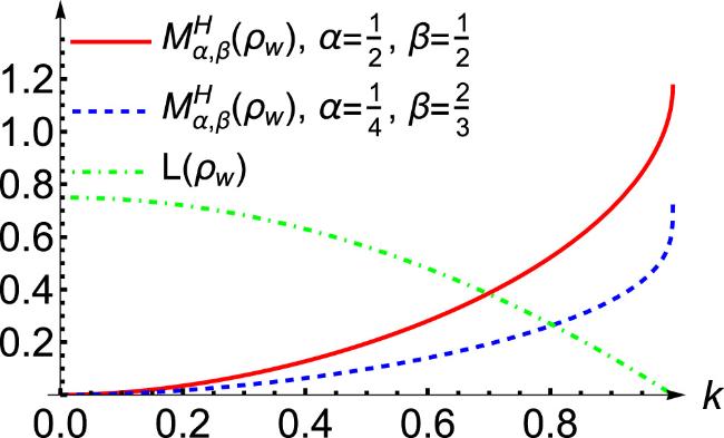
Example 2. Consider the modified Werner state

$\begin{eqnarray}{\rho }_{{\rm{w}}}=\left(\begin{array}{cccc}\frac{1-k}{4} & 0 & 0 & 0\\ 0 & \frac{1+k}{4} & \frac{k}{2}{\rm{i}} & 0\\ 0 & -\frac{k}{2}{\rm{i}} & \frac{1+k}{4} & 0\\ 0 & 0 & 0 & \frac{1-k}{4}\end{array}\right),\end{eqnarray}$
where k ∈ [0, 1]. Note that ρw is a pure state when k=1, ${\rho }_{{\rm{w}}}\in { \mathcal F }$ when k=0 and the eigenvalues of ρw are ${w}_{1}=\frac{1-k}{4}$ and ${w}_{2}=\frac{1+3k}{4}$. By equation (13), we have
$\begin{eqnarray}\begin{array}{l}{M}_{\alpha ,\beta }^{H}({\rho }_{{\rm{w}}})=\frac{1}{(\alpha -1)\beta }\left\{\left[\frac{1}{32}({w}_{1}^{1-\alpha }{w}_{2}^{\alpha }+{w}_{1}^{\alpha }{w}_{2}^{1-\alpha }\right.\right.\\ \quad \left.{\left.\,-\,8({w}_{2}-{w}_{1})+24)\right]}^{\beta }-1\right\}\\ \,=\,\frac{1}{(\alpha -1)\beta }\left\{\left[\frac{1}{8}({(3k+1)}^{\alpha }{(1-k)}^{1-\alpha }\right.\right.\\ \quad \left.{\left.\,+\,{(3k+1)}^{1-\alpha }{(1-k)}^{\alpha }-2k+6)\right]}^{\beta }-1\right\},\end{array}\end{eqnarray}$
for all α ∈ (0, 1) and β ∈ (0, 1].

And the linear entropy (mixedness) of the modified Werner state ρw is $L({\rho }_{{\rm{w}}})=1-{\rm{tr}}{\rho }_{{\rm{w}}}^{2}=3{w}_{1}(1+{w}_{2}-{w}_{1})=\frac{3}{4}(1-{k}^{2})$. We plot the variation of ${M}_{\alpha ,\beta }^{H}({\rho }_{{\rm{w}}})$ and L(ρw) with k in figure 2. Interestingly, ${M}_{\alpha ,\beta }^{H}({\rho }_{{\rm{w}}})$ is increasing with respect to k while L(ρw) is decreasing with respect to k. ${M}_{\alpha ,\beta }^{H}({\rho }_{{\rm{w}}})$ reaches its maximum value of $\frac{1}{(\alpha -1)\beta }(\frac{1}{{2}^{\beta }}-1)$ for any fixed α and β when k=1, in which case L(ρw) reaches its minimum value of 0, while ${M}_{\alpha ,\beta }^{H}({\rho }_{{\rm{w}}})$ reaches its minimum value of 0 when k=0 for any fixed α and β, in which case the linear entropy (mixedness) L(ρw) attains its maximum value of $\frac{3}{4}$.
Figure 2. The variations of ${M}_{\alpha ,\beta }^{H}({\rho }_{{\rm{w}}})$ and L(ρw) with k for fixed α and β. Red solid line fixes $\alpha =\beta =\frac{1}{2}$ in equation (26), while the blue dashed line fixes $\alpha =\frac{1}{4}$ and $\beta =\frac{2}{3}$ in equation (26), and the green dot-dashed line represents L(ρw).
Then consider the modified isotropic state
$\begin{eqnarray}{\rho }_{{\rm{iso}}}=\left(\begin{array}{cccc}\frac{1}{6}(2F+1) & 0 & 0 & \frac{1}{6}(4F-1){\rm{i}}\\ 0 & \frac{1}{3}(1-F) & 0 & 0\\ 0 & 0 & \frac{1}{3}(1-F) & 0\\ -\frac{1}{6}(4F-1){\rm{i}} & 0 & 0 & \frac{1}{6}(2F+1)\end{array}\right),\end{eqnarray}$
where F ∈ [0, 1]. Swapping the position of basis ∣00⟩⟨11∣ with ∣01⟩⟨10∣ and the position of basis ∣11⟩⟨00∣ with ∣10⟩⟨01∣, and setting $F=\frac{3k+1}{4}$, we have ρiso=ρw, i.e, ρiso and ρw are essentially the same state, and we have ${M}_{\alpha ,\beta }^{H}({\rho }_{{\rm{iso}}})={M}_{\alpha ,\beta }^{H}({\rho }_{{\rm{w}}})$ when $F=\frac{3k+1}{4}$.

5. Conclusions

We have proposed two classes of imaginarity monotones induced by the unified (α, β)-relative entropy. The first class of imaginarity monotone ${M}_{\alpha ,\beta }^{H}(\rho )$ is defined by setting σ=ρ*. We have investigated several properties of ${M}_{\alpha ,\beta }^{H}(\rho )$, including superadditivity under direct, subadditivity under tensor product and monotonicity, among others. The second class of imaginarity monotone ${M}_{\alpha ,\beta }^{E}(\rho )$ is defined by minimizing the unified (α, β)-relative entropy over all free states. The properties of ${M}_{\alpha ,\beta }^{E}(\rho )$ exhibit a high degree of similarity to those of ${M}_{\alpha ,\beta }^{H}(\rho )$. Furthermore, we have presented the analytical expressions of ${M}_{\alpha ,\beta }^{H}(\rho )$ for several special quantum states. For ${M}_{\alpha ,\beta }^{E}(\rho )$, we have focused on deriving its analytical expression for qubit states, which differs significantly from the one of ${M}_{\alpha ,\beta }^{H}(\rho )$ under the qubit state case.

Acknowledgments

The authors would like to express their sincere gratitude to the anonymous referees for their useful suggestions which greatly improved this paper. The authors would also like to thank Prof. Jianwei Xu and Lin Zhang for the fruitful discussions. This work was supported by National Natural Science Foundation of China (Grant No. 12161056) and Natural Science Foundation of Jiangxi Province (Grant No. 20232ACB211003).

Appendix A. Proof of Lemma 3

We first prove that $({x}_{0},{\theta }_{0})=\left(\frac{1}{{\left(\frac{A+\sqrt{{B}^{2}+{C}^{2}}}{A-\sqrt{{B}^{2}+{C}^{2}}}\right)}^{\frac{1}{\alpha }}+1},\arcsin \frac{B}{\sqrt{{B}^{2}+{C}^{2}}}\right)$ is the unique extreme point of f(x, θ). In fact, it can be shown that
$\begin{eqnarray*}\begin{array}{rcl}{f}_{x}^{{\prime} }(x,\theta ) & =& A(1-\alpha )\left(\frac{1}{{x}^{\alpha }}-\frac{1}{{(1-x)}^{\alpha }}\right)\\ & & -(B\sin \theta +C\cos \theta )(1-\alpha )\left(\frac{1}{{(1-x)}^{\alpha }}+\frac{1}{{x}^{\alpha }}\right),\end{array}\end{eqnarray*}$
and
$\begin{eqnarray*}\begin{array}{l}{f}_{\theta }^{{\prime} }(x,\theta )=(B\cos \theta -C\sin \theta )\\ \times [{(1-x)}^{1-\alpha }-{x}^{1-\alpha }].\end{array}\end{eqnarray*}$
Letting ${f}_{x}^{{\prime} }(x,\theta )=0$ and ${f}_{\theta }^{{\prime} }(x,\theta )=0$, we obtain that ${x}_{0}=\frac{1}{{\left(\frac{A+\sqrt{{B}^{2}+{C}^{2}}}{A-\sqrt{{B}^{2}+{C}^{2}}}\right)}^{\frac{1}{\alpha }}+1}$, $\sin {\theta }_{0}=\frac{B}{\sqrt{{B}^{2}+{C}^{2}}}$ and $\cos {\theta }_{0}=\frac{C}{\sqrt{{B}^{2}+{C}^{2}}}$, or ${x}_{1}=\frac{1}{{\left(\frac{A-\sqrt{{B}^{2}+{C}^{2}}}{A+\sqrt{{B}^{2}+{C}^{2}}}\right)}^{\frac{1}{\alpha }}+1}$, $\sin {\theta }_{0}=-\frac{B}{\sqrt{{B}^{2}+{C}^{2}}}$ and $\cos {\theta }_{0}=-\frac{C}{\sqrt{{B}^{2}+{C}^{2}}}$. Since $A-\sqrt{{B}^{2}+{C}^{2}}\gt 0$ and ${x}_{0}\in [0,\frac{1}{2}]$, ${x}_{1}\notin [0,\frac{1}{2}]$. Therefore, (x0, θ0) is the unique extreme point of f(x, θ).
Then we prove that (x0, θ0) is the maximum value point of f(x, θ). Direct calculation shows that
$\begin{eqnarray*}\begin{array}{l}{f}_{xx}^{{\prime\prime} }(x,\theta )=-\alpha (1-\alpha )\left[(A-B\sin \theta -C\cos \theta )\frac{1}{{x}^{\alpha +1}}\right.\\ \quad \left.+\,(A+B\sin \theta +C\cos \theta )\frac{1}{{(1-x)}^{\alpha +1}}\right],\end{array}\end{eqnarray*}$
$\begin{eqnarray*}\begin{array}{l}{f}_{x\theta }^{{\prime\prime} }(x,\theta )=-(1-\alpha )(B\cos \theta -C\sin \theta )\\ \quad \times \,\left[\frac{1}{{(1-x)}^{\alpha }}+\frac{1}{{x}^{\alpha }}\right],\end{array}\end{eqnarray*}$
and
$\begin{eqnarray*}\begin{array}{l}{f}_{\theta \theta }^{{\prime\prime} }(x,\theta )=-(B\sin \theta +C\cos \theta )\\ \quad [{(1-x)}^{1-\alpha }-{x}^{1-\alpha }].\end{array}\end{eqnarray*}$
It can be seen that ${f}_{xx}^{{\prime\prime} }({x}_{0},{\theta }_{0})\lt 0$, ${f}_{x\theta }^{{\prime\prime} }({x}_{0},{\theta }_{0})=0$ and ${f}_{\theta \theta }^{{\prime\prime} }({x}_{0},{\theta }_{0})\lt 0$. Therefore, ${[{f}_{x\theta }^{{\prime\prime} }({x}_{0},{\theta }_{0})]}^{2}-{f}_{xx}^{{\prime\prime} }({x}_{0},{\theta }_{0}){f}_{\theta \theta }^{{\prime\prime} }({x}_{0},{\theta }_{0})\lt 0$. Noting that f(x, θ) is a continuous function, we conclude that (x0, θ0) is the maximum value point of f(x, θ). This completes the proof.

Appendix B. Proof of Lemma 4

First of all, since σρ and ${\sigma }_{\tau }\in { \mathcal F }$, we have $p{\sigma }_{\rho }\oplus (1-p){\sigma }_{\tau }\in { \mathcal F }$. Suppose that
$\begin{eqnarray*}\begin{array}{rcl}{M}_{\alpha ,\beta }^{E}(p\rho \displaystyle \oplus (1-p)\tau ) & =& \frac{1}{(\alpha -1)\beta }\\ & & \times \,[{({\rm{tr}}({(p\rho \displaystyle \oplus (1-p)\tau )}^{\alpha }{\sigma }_{0}^{1-\alpha }))}^{\beta }-1].\end{array}\end{eqnarray*}$
Let
$\begin{eqnarray*}{\sigma }_{0}^{1-\alpha }=\left(\begin{array}{cc}{\boldsymbol{S}} & {\boldsymbol{U}}\\ {\boldsymbol{V}} & {\boldsymbol{W}}\end{array}\right).\end{eqnarray*}$
Then we have
$\begin{eqnarray*}\begin{array}{l}{\rm{tr}}({(p\rho \displaystyle \oplus (1-p)\tau )}^{\alpha }{\sigma }_{0}^{1-\alpha })\,\\ \quad =\,\rm{tr}\,\left[\left(\begin{array}{cc}{(p\rho )}^{\alpha } & {\boldsymbol{0}}\\ {\boldsymbol{0}} & {((1-p)\tau )}^{\alpha }\end{array}\right)\left(\begin{array}{cc}{\boldsymbol{S}} & {\boldsymbol{U}}\\ {\boldsymbol{V}} & {\boldsymbol{W}}\end{array}\right)\right]\\ \quad =\,{\rm{tr}}({\boldsymbol{S}}{(p\rho )}^{\alpha }+{\boldsymbol{W}}{((1-p)\tau )}^{\alpha }).\end{array}\end{eqnarray*}$
Therefore, ${\rm{tr}}[{(p\rho \oplus (1-p)\tau )}^{\alpha }{\sigma }_{0}^{1-\alpha }]$ attains its maximum value when ${\boldsymbol{S}}={(p{\sigma }_{\rho })}^{1-\alpha }$ and ${\boldsymbol{W}}={((1-p){\sigma }_{\tau })}^{1-\alpha }$, which is independent of U and V, that is, when
$\begin{eqnarray*}{\sigma }_{0}^{1-\alpha }=\left(\begin{array}{cc}{(p{\sigma }_{\rho })}^{1-\alpha } & {\boldsymbol{0}}\\ {\boldsymbol{0}} & {((1-p){\sigma }_{\tau })}^{1-\alpha }\end{array}\right).\end{eqnarray*}$
Thus, σ0=ρ ⊕ (1-p)στ is a quantum state that reaches the minimum value in equation(20) when the input state is ⊕ (1-p)τ. This completes the proof.

Appendix C. Proof of equation (24)

Let λ1,2=(1 ∓ r)/2 be the eigenvalues of a qubit state ρ, where $r=| \overrightarrow{r}| $. For any qubit free state σ, we assume its Bloch vector is $\overrightarrow{s}=({s}_{1},0,{s}_{3})$, and the eigenvalues of σ are μ1,2=(1 ∓ s)/2, where $s=| \overrightarrow{s}| $. If r=0, it is obvious that ${M}_{\alpha ,\beta }^{E}(\rho )=0$. Now we consider the case of r ≠ 0. It follows from [66] that
$\begin{eqnarray}{\rho }^{\alpha }=\left(\begin{array}{cc}\frac{{\lambda }_{1}^{\alpha }+{\lambda }_{2}^{\alpha }}{2}+\frac{{r}_{3}({\lambda }_{2}^{\alpha }-{\lambda }_{1}^{\alpha })}{2r} & \frac{(-{r}_{1}+{\rm{i}}{r}_{2})({\lambda }_{1}^{\alpha }-{\lambda }_{2}^{\alpha })}{2r}\\ \frac{(-{r}_{1}-{\rm{i}}{r}_{2})({\lambda }_{1}^{\alpha }-{\lambda }_{2}^{\alpha })}{2r} & \frac{{\lambda }_{1}^{\alpha }+{\lambda }_{2}^{\alpha }}{2}-\frac{{r}_{3}({\lambda }_{2}^{\alpha }-{\lambda }_{1}^{\alpha })}{2r}\end{array}\right),\end{eqnarray}$
and
$\begin{eqnarray}{\sigma }^{1-\alpha }=\left(\begin{array}{cc}\frac{{\mu }_{1}^{1-\alpha }+{\mu }_{2}^{1-\alpha }}{2}+\frac{{s}_{3}({\mu }_{2}^{1-\alpha }-{\mu }_{1}^{1-\alpha })}{2s} & \frac{-{s}_{1}({\mu }_{1}^{1-\alpha }-{\mu }_{2}^{1-\alpha })}{2s}\\ \frac{-{s}_{1}({\mu }_{1}^{1-\alpha }-{\mu }_{2}^{1-\alpha })}{2s} & \frac{{\mu }_{1}^{1-\alpha }+{\mu }_{2}^{1-\alpha }}{2}-\frac{{s}_{3}({\mu }_{2}^{1-\alpha }-{\mu }_{1}^{1-\alpha })}{2s}\end{array}\right),\end{eqnarray}$
where s ≠ 0. It implies that
$\begin{eqnarray}\begin{array}{rcl}{\rm{tr}}({\rho }^{\alpha }{\sigma }^{1-\alpha }) & =& \frac{1}{2}({\lambda }_{1}^{\alpha }+{\lambda }_{2}^{\alpha })({\mu }_{1}^{1-\alpha }+{\mu }_{2}^{1-\alpha })\\ & & +\frac{{r}_{3}}{2r}({\lambda }_{2}^{\alpha }-{\lambda }_{1}^{\alpha })\cdot \frac{{s}_{3}}{s}({\mu }_{2}^{1-\alpha }-{\mu }_{1}^{1-\alpha })\\ & & +\frac{{r}_{1}}{2r}({\lambda }_{2}^{\alpha }-{\lambda }_{1}^{\alpha })\cdot \frac{{s}_{1}}{s}({\mu }_{2}^{1-\alpha }-{\mu }_{1}^{1-\alpha }).\end{array}\end{eqnarray}$
Letting $A=\frac{1}{2}({\lambda }_{1}^{\alpha }+{\lambda }_{2}^{\alpha })$, $B=\frac{{r}_{1}}{2r}({\lambda }_{2}^{\alpha }-{\lambda }_{1}^{\alpha })$ and $C\,=\frac{{r}_{3}}{2r}({\lambda }_{2}^{\alpha }-{\lambda }_{1}^{\alpha })$, ${s}_{1}=c\sin \theta $ and ${s}_{3}=c\cos \theta $, where c ∈ [0, 1] and θ ∈ [0, 2π] and $x=\frac{1-c}{2}$, by equation (C3) we have
$\begin{eqnarray}\begin{array}{rcl}{\rm{tr}}({\rho }^{\alpha }{\sigma }^{1-\alpha }) & =& A({x}^{1-\alpha }+{(1-x)}^{1-\alpha })\\ & & +(B\sin \theta +C\cos \theta )[{(1-x)}^{1-\alpha }-{x}^{1-\alpha }].\end{array}\end{eqnarray}$
And when s=0,
$\begin{eqnarray}{\rm{tr}}({\rho }^{\alpha }{\sigma }^{1-\alpha })=\frac{{\lambda }_{1}^{\alpha }+{\lambda }_{2}^{\alpha }}{{2}^{1-\alpha }}.\end{eqnarray}$
If B2 + C2=0, we have ${\rm{tr}}{({\rho }^{\alpha }{\sigma }^{1-\alpha })}_{{\rm{\max }}}={\rm{\max }}\{A({x}^{1-\alpha }+{(1-x)}^{1-\alpha }),({\lambda }_{1}^{\alpha }+{\lambda }_{2}^{\alpha })/{2}^{1-\alpha }\}$. Direct calculation shows that ${\rm{tr}}({\rho }^{\alpha }{\sigma }^{1-\alpha })$ achieves its maximum value of 2αA when s1=s3=0. In this case, ${M}_{\alpha ,\beta }^{E}(\rho )\,=\frac{1}{(\alpha -1)\beta }({2}^{\alpha \beta }{A}^{\beta }-1)$.
If B2+C2 > 0, we have ${\left(\frac{1}{2}\right)}^{1-\alpha }({\lambda }_{1}^{\alpha }+{\lambda }_{2}^{\alpha })$ $\leqslant {\rm{\max }}\{A({x}^{1-\alpha }\,+{(1-x)}^{1-\alpha })+(B\sin \theta +C\cos \theta )[{(1-x)}^{1-\alpha }-{x}^{1-\alpha }]\}$. So ${\rm{tr}}({\rho }^{\alpha }{\sigma }^{1-\alpha })$ achieves its maximum value when s ≠ 0. Note that $x\in [0,\frac{1}{2}]$, $A\gt \sqrt{{B}^{2}+{C}^{2}}$, B2+C2 > 0 and α ∈ (0, 1). It follows from Lemma 3 that ${\rm{tr}}({\rho }^{\alpha }{\sigma }^{1-\alpha })$ reaches its maximum value at $({x}_{0},{\theta }_{0})=\left(\frac{1}{{\left(\frac{A+\sqrt{{B}^{2}+{C}^{2}}}{A-\sqrt{{B}^{2}+{C}^{2}}}\right)}^{\frac{1}{\alpha }}+1},\arcsin \frac{B}{\sqrt{{B}^{2}+{C}^{2}}}\right)$ and the maximum value is
$\begin{eqnarray}\begin{array}{rcl}{\rm{tr}}{({\rho }^{\alpha }{\sigma }^{1-\alpha })}_{\max } & =& (A+\sqrt{{B}^{2}+{C}^{2}})\\ & & \times {\left(1-\frac{1}{{\left(\frac{A+\sqrt{{B}^{2}+{C}^{2}}}{A-\sqrt{{B}^{2}+{C}^{2}}}\right)}^{\frac{1}{\alpha }}+1}\right)}^{1-\alpha }\\ & & +(A-\sqrt{{B}^{2}+{C}^{2}}){\left(\frac{1}{{\left(\frac{A+\sqrt{{B}^{2}+{C}^{2}}}{A-\sqrt{{B}^{2}+{C}^{2}}}\right)}^{\frac{1}{\alpha }}+1}\right)}^{1-\alpha },\end{array}\end{eqnarray}$
when s ≠ 0.
Since α ∈ (0, 1) and β ∈ (0, 1], it is obvious that ${M}_{\alpha ,\beta }^{E}(\rho )$ reaches its minimum value when ${\rm{tr}}({\rho }^{\alpha }{\sigma }^{1-\alpha })$ reaches its maximum value. By equation (C6) and equation (20), we obtain equation (24). When ${x}_{0}=\frac{1}{{\left(\frac{A+\sqrt{{B}^{2}+{C}^{2}}}{A-\sqrt{{B}^{2}+{C}^{2}}}\right)}^{\frac{1}{\alpha }}+1}$, we have ${c}_{0}=1-2{x}_{0}=1-\frac{2}{{\left(\frac{A+\sqrt{{B}^{2}+{C}^{2}}}{A-\sqrt{{B}^{2}+{C}^{2}}}\right)}^{\frac{1}{\alpha }}+1}$, which implies that ${\rm{tr}}({\rho }^{\alpha }{\sigma }^{1-\alpha })$ reaches its maximum value, and thus equation (20) reaches its minimum value for qubit free state when ${s}_{1}={c}_{0}\sin {\theta }_{0}=\left(1-\frac{2}{{\left(\frac{A+\sqrt{{B}^{2}+{C}^{2}}}{A-\sqrt{{B}^{2}+{C}^{2}}}\right)}^{\frac{1}{\alpha }}+1}\right)\frac{B}{\sqrt{{B}^{2}+{C}^{2}}}$ and ${s}_{3}={c}_{0}\cos {\theta }_{0}=-\left(1-\frac{2}{{\left(\frac{A+\sqrt{{B}^{2}+{C}^{2}}}{A-\sqrt{{B}^{2}+{C}^{2}}}\right)}^{\frac{1}{\alpha }}+1}\right)\frac{C}{\sqrt{{B}^{2}+{C}^{2}}}$. Note that the value of ${\rm{tr}}{({\rho }^{\alpha }{\sigma }^{1-\alpha })}_{{\rm{\max }}}$ when B2+C2=0 is equal to the value of ${\rm{tr}}{({\rho }^{\alpha }{\sigma }^{1-\alpha })}_{{\rm{\max }}}$ when B2+C2 ≠ 0. This completes the proof.
1
Namiki M, Pascazio S 1991 Wave-function collapse by measurement and its simulation Phys. Rev. A 44 39

DOI

2
Ricardo K 2020 Why are complex numbers needed in quantum mechanics? Some answers for the introductory level Am. J. Phys. 88 39

DOI

3
David G 2018 Connection formulas between Coulomb wave functions J. Math. Phys. 59 112104

DOI

4
Adler S L, Millard A C 1996 Generalized quantum dynamics as pre-quantum mechanics Nucl. Phys. B 473 199

DOI

5
Rochon D, Tremblay S 2004 Bicomplex quantum mechanics: I. The generalized Schrödinger equation Adv. Appl. Clifford Al. 14 231

DOI

6
Lahoz-Beltra R 2022 Solving the Schrödinger equation with genetic algorithms: a practical approach Computers 11 169

DOI

7
Jumarie G 2001 Schrödinger equation for quantum fractal space-time of order n via the complex-valued fractional Brownian motion Int. J. Mod. Phys. A 16 5061

DOI

8
Bernstein S 2006 Factorization of the nonlinear Schrödinger equation and applications Complex. Var. Elliptic. Equ. 51 429

DOI

9
Hu Y, Kallianpur G 2000 Schrödinger equations with fractional Laplacians Appl. Math. Opt. 42 281

DOI

10
Rochon D 2008 On a relation of bicomplex pseudoanalytic function theory to the complexified stationary Schrödinger equation Complex. Var. Elliptic. Equ. 53 501

DOI

11
Dong J, Xu M 2008 Space-time fractional Schrödinger equation with time-independent potentials J. Math Anal. Appl. 344 1005

DOI

12
Bialynicki-Birula I 1996 V photon wave function Prog. Opt. 36 245

DOI

13
Karama R 2020 Schrödinger's original struggles with a complex wave function Am. J. Phys. 88 433

DOI

14
Sawada S I, Heather R, Jackson B, Metiu H 1985 A strategy for time dependent quantum mechanical calculations using a Gaussian wave packet representation of the wave function J. Chem. Phys. 83 3009

DOI

15
Aronstein D L, Stroud C R 1997 Fractional wave-function revivals in the infinite square well Phys. Rev. A 55 4526

DOI

16
Heather R, Metiu H 1987 An efficient procedure for calculating the evolution of the wave function by fast Fourier transform methods for systems with spatially extended wave function and localized potential J. Chem. Phys. 86 5009

DOI

17
Shestakova T P 2019 On the meaning of the wave function of the Universe Int. J. Mod. Phys. D 28 1941009

DOI

18
Abedi A, Maitra N T, Gross E K U 2010 Exact factorization of the time-dependent electron-nuclear wave function Phys. Rev. Lett. 105 123002

DOI

19
Fried D L 2001 Adaptive optics wave function reconstruction and phase unwrapping when branch points are present Opt. Commun. 200 43

DOI

20
Huang Z, Balatsky A V 2016 Dynamical quantum phase transitions: role of topological nodes in wave function overlaps Phys. Rev. Lett. 117 086802

DOI

21
Simsarian J E, Denschlag J, Edwards M, Clark C W, Deng L, Hagley E W, Helmerson K, Rolston S L, Phillips W D 2000 Imaging the phase of an evolving Bose-Einstein condensate wave function Phys. Rev. Lett. 85 2040

DOI

22
Wernsdorfer W, Sessoli R 1999 Quantum phase interference and parity effects in magnetic molecular clusters Science 284 133

DOI

23
Pan X, Schwinger J, Huang N, Song P, Chua W, Hanamura F, Joshi A, Valadares F, Filip R, Gao Y 2023 Protecting the quantum interference of cat states by phase-space compression Phys. Rev. X 13 021004

DOI

24
Zhang Y, Wei K, Xu F 2020 Generalized Hong-Ou-Mandel quantum interference with phase-randomized weak coherent states Phys. Rev. A 101 033823

DOI

25
Nsofini J, Ghofrani K, Sarenac D, Cory D G, Pushin D A 2016 Quantum-information approach to dynamical diffraction theory Phys. Rev. A 94 062311

DOI

26
Karan S 2022 Superconducting quantum interference at the atomic scale Nat. Phys. 18 893

DOI

27
Qian K, Wang K, Chen L, Hou Z, Krenn M, Zhu S, Ma X 2023 Multiphoton non-local quantum interference controlled by an undetected photon Nat. Commun. 14 1480

DOI

28
Hogg T 1996 Quantum computing and phase transitions in combinatorial search J. Artif. Intell. Res. 4 91

DOI

29
Troppmann U, Gollub C, Vivie-Riedle R 2006 The Role of phases and their interplay in molecular vibrational quantum computing with multiple qubits New J. Phys. 8 100

DOI

30
Wetering J 2020 ZX-calculus for the working quantum computer scientist arXiv:2012.13966

31
Hu X 2020 Experimental high-dimensional quantum teleportation Phys. Rev. Lett. 125 230501

DOI

32
Cacciapuoti A S, Caleffi M, Meter R V, Hanzo L 2020 When entanglement meets classical communications: quantum teleportation for the quantum internet IEEE T. Commun. 68 3808

DOI

33
Chen M, Li R, Gan L, Zhu X, Yang G, Lu C, Pan J 2020 Quantum-teleportation-inspired algorithm for sampling large random quantum circuits Phys. Rev. Lett. 124 080502

DOI

34
Bassi A, Lochan K, Satin S, Singh T P, Ulbricht H 2013 Models of wave-function collapse, underlying theories, and experimental tests Rev. Mod. Phys. 85 471

DOI

35
Tsallis C 1994 What are the numbers that experiments provide Quim Nova 17 468

36
Procopio L M, Rozema L A, Wong Z J, Hamel D R, O'Brien K, Zhang X, Dakić B, Walther P 2017 Single-photon test of hyper-complex quantum theories using a metamaterial Nat. Commun. 8 15044

DOI

37
Wu D 2022 Experimental refutation of real-valued quantum mechanics under strict locality conditions Phys. Rev. Lett. 129 140401

DOI

38
Adler S L 2017 Peres experiment using photons: no test for hypercomplex (quaternionic) quantum theories Phys. Rev. A 95 060101

DOI

39
Jacak M M, Jówiak P, Niemczuk J, Jacak J E 2021 Quantum generators of random numbers Sci. Rep. 11 16108

DOI

40
Raymer M G 1997 Measuring the quantum mechanical wave function Contemp. Phys. 38 343

DOI

41
Remez R, Karnieli A, Trajtenberg-Mills S, Shapira N, Kaminer I, Lereah Y, Arie A 2019 Observing the quantum wave nature of free electrons through spontaneous emission Phys. Rev. Lett. 123 060401

DOI

42
Weinberg S 1989 Testing quantum mechanics Ann. Phys. 194 336

DOI

43
Hickey A, Gour G 2018 Quantifying the imaginarity of quantum mechanics J. Phys. A-Math. Theor. 51 414009

DOI

44
Wu K, Kondra T V, Rana S, Scandolo C M, Xiang G, Li C, Guo G, Streltsov A 2021 Operational resource theory of imaginarity Phys. Rev. Lett. 126 090401

DOI

45
Xue S, Guo J, Li P, Ye M, Li Y 2021 Quantification of resource theory of imaginarity Quantum Inf. Process. 20 383

DOI

46
Wu K, Kondra T V, Rana S, Scandolo C M, Xiang G, Li C, Guo G, Streltsov A 2021 Resource theory of imaginarity: quantification and state conversion Phys. Rev. A 103 032401

DOI

47
Chen Q, Gao T, Yan F 2023 Measures of imaginarity and quantum state order Sci. China Phys. Mech. Astron. 66 280312

DOI

48
Guo M, Li B, Fei S-M 2025 Geometric-like imaginarity: quantification and state conversion Sci. China Phys. Mech. Astron. 68 220311

DOI

49
Xu J 2024 Quantifying the imaginarity of quantum states via Tsallis relative entropy Phys. Lett. A 528 130024

DOI

50
Chen X, Lei Q 2024 Imaginarity measure induced by relative entropy arXiv:2404.00637

51
Xu J 2023 Imaginarity of Gaussian states Phys. Rev. A 108 062203

DOI

52
Fan Y, Guo Z, Liu Y, Cao H 2024 Resource theory of Kirkwood-Dirac imaginarity Phys. Scr. 99 085115

DOI

53
Wu K, Kondra T V, Scandolo C M, Rana S, Xiang G, Li C, Guo G, Streltsov A 2024 Resource theory of imaginarity in distributed scenarios Commun. Phys. 7 171

DOI

54
Bromley T R, Cianciaruso M, Adesso G 2015 Frozen quantum coherence Phys. Rev. Lett. 114 210401

DOI

55
Mondal D, Pramanik T, Pati A K 2017 Nonlocal advantage of quantum coherence Phys. Rev. A 95 010301

DOI

56
Han S, Zheng B, Guo Z 2024 Freezing imaginarity of quantum states based on l1-norm Chin. Phys. B 33 100306

DOI

57
Wei Z, Fei S-M 2024 Nonlocal advantages of quantum imaginarity Phys. Rev. A 110 052202

DOI

58
Zhang L, Li N 2024 Coherence as maximal imaginarity generated by incoherent operations Europhys. Lett. 148 28002

DOI

59
Zhang L, Li N 2024 Can imaginarity be broadcast via real operations? Commun. Theor. Phys. 76 115104

DOI

60
Wang J, Wu J, Minhyung C 2011 Unified (r, s)-relative entropy Int. J. Theor. Phys. 50 1282

DOI

61
Miszczak J A, Pucha&Lstrok;a Z, Horodecki P, Uhlmann A, Zyczkowski K 2009 Sub-and super-fidelity as bounds for quantum fidelity Quantum Inf. Comput. 9 103

DOI

62
Baumgratz T, Cramer M, Plenio M B 2014 Quantifying coherence Phys. Rev. Lett. 113 140401

DOI

63
Yu X, Zhang D, Xu G, Tong D 2016 Alternative framework for quantifying coherence Phys. Rev. A 94 060302

DOI

64
Baek K, Sohbi A, Lee J, Kim J, Nha H 2020 Quantifying coherence of quantum measurements New J. Phys. 22 093019

DOI

65
Mu H, Li Y 2020 Quantum uncertainty relations of two quantum relative entropies of coherence Phys. Rev. A 102 022217

DOI

66
Xu C, Wu Z, Fei S-M 2022 Uncertainty of quantum channels via modified generalized variance and modified generalized Wigner-Yanase-Dyson skew information Quantum Inf. Process. 21 292

DOI

Outlines

/