


1. Introduction
The Husimi function (Q-function) [1] of a quantum state described by the density operator $\hat{\rho }$, is the distribution function in the coherent state representation. For instance, the Husimi function of a harmonic oscillator and a spin-1/2 particle can be expressed as $\langle {\boldsymbol{\alpha }}| \hat{\rho }| {\boldsymbol{\alpha }}\rangle /\pi $ and $\langle {\boldsymbol{n}}| \hat{\rho }| {\boldsymbol{n}}\rangle /2\pi $, respectively. Here {∣α⟩} are the coherent states of this harmonic oscillator, and {∣n⟩} are the SU(2) spin-coherent states. The Husimi function has broad applications in various directions of quantum physics, e.g., quantum optics and quantum precise measurement.
The Wehrl entropy of a quantum state $\hat{\rho }$ is the Shannon entropy of the corresponding Husimi function [2]. The Wehrl entropy has been extensively studied in mathematical physics [3-6] and quantum chaos [7]. For many-body spin systems, it is also found that this entropy can be used as a measurement of the complexity of many-body entanglement [5,8].
Here, we investigate the statistical interpretation of the Husimi function and Wehrl entropy. We take the system of N spin-1/2 particles as an example.
Since the coherent states are not a group of the orthonormal basis of the Hilbert space, the Husimi function cannot be directly interpreted as the probability distribution of the measurement outcomes of a certain observable. Thus, the Wehrl entropy cannot be directly interpreted as the entropy corresponding to such a probability distribution, which distinguishes it from the more commonly used von Neumann entropy. However, due to the completeness relation of the coherent states, i.e., $\int {\rm{d}}{\boldsymbol{n}}| {\boldsymbol{n}}\rangle \langle {\boldsymbol{n}}| /Z=\hat{I}$, with Z being a constant, the projection operators {∣n⟩⟨n∣} of the coherent states form a positive operator-valued measurement (POVM). Explicitly [9], one can implement this POVM (i.e., realize a measurement with the probability distribution of the possible results being same as the Husimi function) by first entangling the quantum systems with an ancillary system, and then measuring the ancillary system. Such a realization of the POVM can be understood as a statistical interpretation of the Husimi function. For systems with continuous variables, such as photons, this implementation of POVM has been demonstrated in various experiments using heterodyne detection [10,11].
In this work, using the Bayes theorem we provide an alternative probabilistic interpretation for the Husimi function and the Wehrl entropy, which has the following two characteristics:
| (1) Our interpretation is based on the direct measurement of the quantum system. The aforementioned ancillary system of the POVM is not required. | |
| (2) More importantly, under this interpretation, the classical correspondence of the Husimi function is exactly the Liouville function (phase-space probability distribution function) of N classical tops, and thus the one of the Wehrl entropy is the Gibbs entropy of these tops, respectively. |
Therefore, our probabilistic interpretation provides a more intuitive understanding of Husimi function and Wehrl entropy. This statistical interpretation can be generalized to the continuous-variable systems. As mentioned before, Husimi function and Wehrl entropy are widely used in the research of various quantum systems. Thus, our results are helpful for understanding the properties of these systems, which are described by the Husimi function and Wehrl entropy. Moreover, these results also enhance our comprehension of the relationship between the Husimi function, Wehrl entropy, and the classical-quantum correspondence.
The remainder of this paper is as follows. In section 2 , we introduce the definitions of the Husimi function and Wehrl entropy of N spin-1/2 particles. The statistical interpretation of the Wehrl entropy is given in section 3 . In section 4 , we describe the classical correspondence of the statistical interpretation of the Husimi function and Wehrl entropy of spin-1/2 particles. In section 5 , we generalize the statistical interpretation to continuous-variable systems. A summary of our results is given in section 6 , and some details of the calculation are given in the Appendix.
2. The Husimi function and Wehrl entropy of spin particles
We consider a system of N spin-1/2 particles labeled as 1, …, N. A spin coherent state can be written as the direct product of the spin-coherent states for each individual particle
$\begin{eqnarray}| {\boldsymbol{n}}\rangle \equiv | {{\boldsymbol{n}}}_{1}{\rangle }_{1}\otimes | {{\boldsymbol{n}}}_{2}{\rangle }_{2}\otimes ...\otimes | {{\boldsymbol{n}}}_{N}{\rangle }_{N},\end{eqnarray}$
with n ≡ (n1, n2, …, nN) ∈ S2⨂N, where nj denotes a unit vector in three-dimensional space, corresponding to a point on the unit sphere (also known as the Bloch sphere), S2, with j=1, …, N. The unit vector can be expressed in spherical coordinates as ${{\boldsymbol{n}}}_{j}=(\sin {\theta }_{j}\cos {\phi }_{j},\sin {\theta }_{j}\sin {\phi }_{j},\cos {\theta }_{j})$, where θj ∈ [0, π] and Φj ∈ [0, 2π]. In addition, S2⨂N represents the Cartesian product of N unit spheres.Furthermore, ∣nj⟩j is the spin-coherent state of the jth particle oriented along the direction nj, which have two eigenvalues ± 1 and corresponding eigenstates,
$\begin{eqnarray}\left[{\hat{{\boldsymbol{\sigma }}}}^{(j)}\cdot {{\boldsymbol{n}}}_{j}\right]| \,\pm {{\boldsymbol{n}}}_{j}{\rangle }_{j}=\pm | \pm {{\boldsymbol{n}}}_{j}{\rangle }_{j},\end{eqnarray}$
where ${\hat{{\boldsymbol{\sigma }}}}^{(j)}=({\hat{\sigma }}_{x}^{(j)},{\hat{\sigma }}_{y}^{(j)},{\hat{\sigma }}_{z}^{(j)})$, with ${\hat{\sigma }}_{x,y,z}^{(j)}$ being the Pauli operators associated with particle j (j=1, …, N). Although the spin coherent states {∣n⟩} are not orthogonal, they satisfy the overcomplete relation $\begin{eqnarray}\frac{1}{{(2\pi )}^{N}}\int {\rm{d}}{\boldsymbol{n}}| {\boldsymbol{n}}\rangle \langle {\boldsymbol{n}}| =\hat{I},\end{eqnarray}$
where $\hat{I}$ is the unit operator, and the integral of n can be written as $\begin{eqnarray}\int {\rm{d}}{\boldsymbol{n}}=\displaystyle \prod _{j=1}^{N}{\int }_{0}^{2\pi }{\rm{d}}{\phi }_{j}{\int }_{0}^{\pi }\sin {\theta }_{j}{\rm{d}}{\theta }_{j}.\end{eqnarray}$
The Husimi function ${P}_{H}(\hat{\rho };{\boldsymbol{n}})$ of this system is defined as
$\begin{eqnarray}{P}_{H}(\hat{\rho };{\boldsymbol{n}})\equiv \frac{1}{{(2\pi )}^{N}}\langle {\boldsymbol{n}}| \hat{\rho }| {\boldsymbol{n}}\rangle ,\end{eqnarray}$
where $\hat{\rho }$ is the density matrix representing the quantum state of the N particles. Unlike the Wigner W-distribution, the Husimi function is both non-negative and bounded, which follows that $0\leqslant {P}_{H}(\hat{\rho };{\boldsymbol{n}})\leqslant 1/(2\pi )$ for any n. Moreover, the Husimi function ${P}_{H}(\hat{\rho };{\boldsymbol{n}})$ is normalized to unity $\begin{eqnarray}\int {\rm{d}}{\boldsymbol{n}}{P}_{H}(\hat{\rho };{\boldsymbol{n}})=1.\end{eqnarray}$
Each Husimi function ${P}_{H}(\hat{\rho };{\boldsymbol{n}})$ uniquely corresponds to an N-particle quantum state $\hat{\rho }$. Specifically, if $\hat{\rho }\ne {\hat{\rho }}^{{\prime} }$, there must exist a direction n ∈ S2⨂N such that ${P}_{H}(\hat{\rho };{\boldsymbol{n}})\ne {P}_{H}({\hat{\rho }}^{{\prime} };{\boldsymbol{n}})$.The Wehrl entropy for this system of N spin-1/2 particles is defined as the entropy associated with the Husimi function
$\begin{eqnarray}{S}_{W}(\hat{\rho })\equiv -\int {P}_{H}(\hat{\rho };{\boldsymbol{n}})\mathrm{ln}\left[{P}_{H}(\hat{\rho };{\boldsymbol{n}})\right]{\rm{d}}{\boldsymbol{n}}.\end{eqnarray}$
Obviously, the Wehrl entropy is a functional of the quantum state $\hat{\rho }$, and it is in the form of the Shannon entropy of the Husimi function.3. The statistical interpretation of the Husimi function and the Wehrl entropy
In this section we demonstrate the statistical interpretation of the Husimi function and the Wehrl entropy.
Since the coherent states ∣n⟩ and $| {{\boldsymbol{n}}}^{{\prime} }\rangle $ defined above are not orthogonal if $\langle {{\boldsymbol{n}}}_{j}^{{\prime} }| {{\boldsymbol{n}}}_{j}\rangle \ne 0$ for all j=1, …, N, these states are not eigenstates of the same observable. Consequently, the Husimi function ${P}_{H}(\hat{\rho };{\boldsymbol{n}})$ cannot be interpreted as the probability distribution of the outcome of a measurement for any specific observable. Hence, the Wehrl entropy cannot be directly interpreted as the entropy of such a probability distribution.
Here we provide a statistical interoperation for the Husimi function and the Wehrl entropy. We will demonstrate that they can still be interpreted as a certain well-defined probability distribution with a clear physical meaning, and the corresponding entropy, respectively.
We begin from the single-particle case (N=1). Consider the following thought experiment: assume there are m copies c(1), c(2), …, c(m) of the spin-1/2 particle, with each one being in the same state $\hat{\rho }$. In addition, the experimenter generates m independent random unit vectors u(1), u(2), …, u(m) from the unit sphere S2. Explicitly, the probability densities of these vectors in S2 are all 1/(4π), and are independent of each other. Then the experimenter performs the following m steps: in the η-th step (η=1, …, m), the experimenter measures the Pauli operator vector $\hat{{\boldsymbol{\sigma }}}$ along the direction u(η) (i.e., the observable $\hat{{\boldsymbol{\sigma }}}\cdot {{\boldsymbol{u}}}^{(\eta )}$) for the copy c(η). If and only if the outcome of this measurement is +1, the experimenter notes down the direction u(η) in a notebook. In figure 1, we schematically illustrate these m steps.
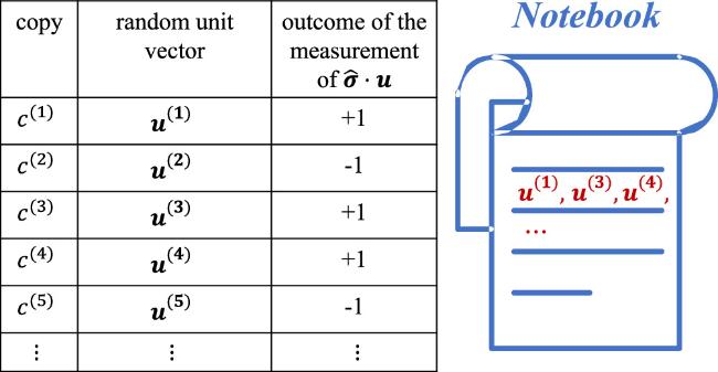
Figure 1. A schematic illustration of the thought experiment of section |
We consider the cases where m is very large, and assume that when all these m steps are finished, there are D directions noted down in the notebook. Then, the following question arises:
Question: What is the distribution of the directions noted down in the notebook? In other words, for a given direction n ∈ S2, how many directions, among the D ones in the notebook, are in a small solid angle ΔΩ around n?
This question can be answered as follows:
Answer: Denote the answer to the above question (i.e., the number of directions in the region described above) as ${ \mathcal N }({\boldsymbol{n}})$. Since a direction can be noted down in the notebook, if and only if the outcome of the corresponding measurement is +1, the answer to the above question can be expressed as:
$\begin{eqnarray}{ \mathcal N }({\boldsymbol{n}})=D{ \mathcal P }\left({\boldsymbol{n}}\left|\right.+1\right){\rm{\Delta }}{\rm{\Omega }}.\end{eqnarray}$
Here, ${ \mathcal P }\left({\boldsymbol{n}}\left|\right.+1\right)$ is a conditional probability density, i.e., the probability density of a randomly-chosen direction being n, under the condition that the outcome of the measurement of the $\hat{{\boldsymbol{\sigma }}}$-operator along that direction is +1.Moreover, according to the Bayes' theorem, we have
$\begin{eqnarray}{ \mathcal P }\left({\boldsymbol{n}}\left|\right.+1\right)=\frac{{ \mathcal P }\left(+1\left|\right.{\boldsymbol{n}}\right)}{{ \mathcal P }\left(+1\right)}{ \mathcal P }\left({\boldsymbol{n}}\right).\end{eqnarray}$
Here, ${ \mathcal P }\left({\boldsymbol{n}}\right)=1/(4\pi )$ is the probability density of a randomly-chosen direction being n, ${ \mathcal P }\left(+1| {\boldsymbol{n}}\right)$ is the probability that the outcome of the measurement of the σ-operator along this random-chosen direction is +1 and can be expressed as $\begin{eqnarray}{ \mathcal P }\left(+1\left|\right.{\boldsymbol{n}}\right)=\langle {\boldsymbol{n}}| \hat{\rho }| {\boldsymbol{n}}\rangle ,\end{eqnarray}$
and ${ \mathcal P }(+1)=\int {\rm{d}}{{\boldsymbol{n}}}^{{\prime} }{ \mathcal P }(+1\left|\right.{{\boldsymbol{n}}}^{{\prime} }){ \mathcal P }({{\boldsymbol{n}}}^{{\prime} }).$Since both ${ \mathcal P }\left({\boldsymbol{n}}\right)$ and ${ \mathcal P }\left(+1\right)$ are independent of n, equations (9 , 10 ) yield that ${ \mathcal P }\left({\boldsymbol{n}}\left|\right.+1\right)=Z\langle {\boldsymbol{n}}| \hat{\rho }| {\boldsymbol{n}}\rangle ,$ with the constant Z being determined by the normalization condition $\int {\rm{d}}{\boldsymbol{n}}{ \mathcal P }\left({\boldsymbol{n}}\left|\right.+1\right)=1$. The direct calculation gives Z=1/(2π). Therefore, we finally obtain ${ \mathcal P }\left({\boldsymbol{n}}\left|\right.+1\right)=\langle {\boldsymbol{n}}| \hat{\rho }| {\boldsymbol{n}}\rangle /(2\pi )$, or 8 ), we find that the amount of the noted-down directions in the small solid angle ΔΩ among n is:
$\begin{eqnarray}{ \mathcal P }\left({\boldsymbol{n}}\left|\right.+1\right)={P}_{H}(\hat{\rho };{\boldsymbol{n}}).\end{eqnarray}$
Substituting this result into equation ( $\begin{eqnarray}{ \mathcal N }({\boldsymbol{n}})=D{P}_{H}(\hat{\rho };{\boldsymbol{n}}){\rm{\Delta }}{\rm{\Omega }}.\end{eqnarray}$
That is the answer to the question.From the above discussion, we know that the Husimi function ${P}_{H}(\hat{\rho };{\boldsymbol{n}})$ can be interpreted as the conditional probability density ${ \mathcal P }\left({\boldsymbol{n}}\left|\right.+1\right)$. Moreover, in the above thought experiment with m →∞, we can consider the directions noted down in the notebook as an ensemble of directions in S2, and the probability distribution corresponding to this ensemble is just ${P}_{H}(\hat{\rho };{\boldsymbol{n}})$.
Additionally, the Husimi function ${P}_{H}(\hat{\rho };{\boldsymbol{n}})$ can also be interpreted with another thought experiment, which is similar to the above one. As above, the experimenter also prepares m copies and performs m measurements on the observable $\hat{{\boldsymbol{\sigma }}}\cdot {{\boldsymbol{u}}}^{(\eta )}(\eta =1,\ldots ,\,m)$, and notes down the direction u(η) in the notebook if the outcome is +1. Nevertheless, if the outcome is -1, the experimenter records the direction -u(η) in the notebook, rather than just ignoring it as in the above thought experiment, as shown in figure 2. With similar calculations as above, we can prove that for m →∞ the distribution of the directions in the notebook still satisfies equation (12 ), i.e., is proportional to the Husimi function.
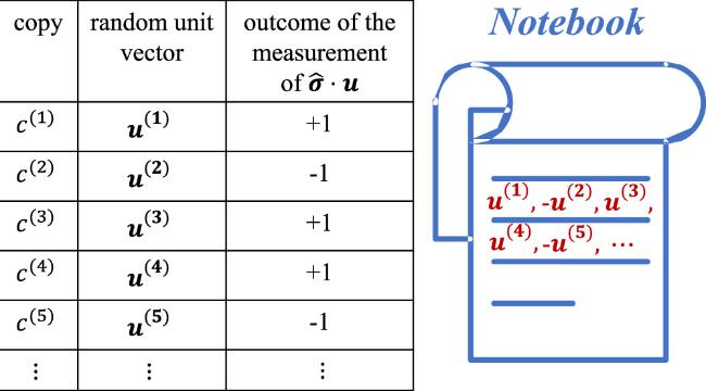
Figure 2. A schematic illustration of the second thought experiment of section |
For convenience, our following discussions are all based on the first thought experiment (i.e., the one of figure 1).
The above discussions can be straightforwardly generalized to the multi-particle (N > 1) cases. In the thought experiment of these cases, each copy c(η) (η=1, …, m) includes N particles, and every copy has the same N-body density operator $\hat{\rho }$. In addition, each u(η)(η=1, …, m) is randomly selected from S2⨂N, and includes N component with each one being in S2, i.e., ${{\boldsymbol{u}}}^{(\eta )}\equiv ({{\boldsymbol{u}}}_{1}^{(\eta )},\ldots ,{{\boldsymbol{u}}}_{N}^{(\eta )})$ with ${{\boldsymbol{u}}}_{j}^{(\eta )}\in {S}^{2}$ (j=1, …, N). As before, the thought experiment includes m steps of measurement and noting. Nevertheless, now in the η-th step (η=1, …, m), the experimenter needs to measure N observables, i.e., measure the value of $\hat{{\boldsymbol{\sigma }}}\cdot {{\boldsymbol{u}}}_{j}^{(\eta )}$ of the j-th particle of the copy c(η), for all j=1, …, N. The experimenter notes down u(η) in the notebook, if and only if the outcomes of these N measurements are all +1.
As in the single-particle case, here we can still prove the relation of equation (11 ), while now n ≡ (n1, …, nN) ∈ S2⨂N, with nj ∈ S2 (j=1, …, N). Therefore, for arbitrary particle number N, the Husimi function ${P}_{H}(\hat{\rho };{\boldsymbol{n}})$ can always be interpreted as ${ \mathcal P }\left({\boldsymbol{n}}\left|\right.+1\right)$, i.e., the probability density of a randomly-chosen element of S2⨂N being n, under the condition that the outcomes of the measurements of $\hat{{\boldsymbol{\sigma }}}\cdot {{\boldsymbol{n}}}_{j}$ of the particle j for each particle j (j=1, …, N) are all +1. Clearly, it is also the distribution of the u-vectors noted down in the thought experiment in the limit m →∞.
Furthermore, according to the above statistical interpretation of the Husimi function ${P}_{H}(\hat{\rho };{\boldsymbol{n}})$, the Wehrl entropy can be interpreted as the entropy corresponding to the conditional probability density ${ \mathcal P }\left({\boldsymbol{n}}\left|\right.+1\right)$ of our system, or the entropy corresponding to the distribution of the u-vectors noted down in the thought experiment, in the limit that there are infinity copies.
So far we have obtained the statistical interoperation of the Husimi function and Wehrl entropy of the N quantum spin-1/2 particles. In section 4 , we explore the classical correspondence of the above interpretation of the Wehrl entropy of spin-1/2 particles. Precisely speaking, spin-1/2 particles constitute a pure quantum system and do not have exact classical correspondences. Nevertheless, as described in section 4 , precessing symmetric spinning tops can be viewed as a classical analogy of spin-1/2 particles. By calculating the related probabilities, we demonstrate that in this analogy, the Wehrl entropy of N quantum spin-1/2 particles corresponds to the Gibbs entropy of N such classical tops.
4. Classical correspondence of the Husimi function and Wehrl entropy
In this section we study the classical correspondence of the statistical interpretation of the Husimi function and Wehrl entropy of spin-1/2 particles, which are given in section 3 .
As in that section, we begin from the single-particle (N=1) case. Precisely speaking, a spin-1/2 particle is a pure quantum system and does not have exact classical correspondence. Nevertheless, we can still find ‘classical analogies' for this kind of particle, i.e., classical systems with dynamic equations being equivalent to the Heisenberg equations of a spin-1/2 particle.
In figure 3(a), we present one example of such systems: a charged axial symmetric top precessing in a homogeneous magnetic field. Explicitly, the top is rapidly spinning along its symmetry axis with fixed angular speed ω, and the center-of-mass of this top is fixed in an inertial frame of reference. In addition, an electric charge Q is fixed on the edge of the top, forming an electric current during the spinning. Due to this current, the top gains a magnetic moment, and thus is subject to a force moment from the magnetic field. The precession of this top, i.e., the changing of the direction of the symmetry axis of the top in the inertial frame of reference, is caused by this force moment. When the spinning is rapid enough, the unit vector w along the symmetry axis of the top satisfies the dynamical equation during the precession (Appendix A ).13 ) of the above charged spinning top in a magnetic field B=-2f/C.
$\begin{eqnarray}\frac{{\rm{d}}{\boldsymbol{w}}}{{\rm{d}}t}=C{\boldsymbol{w}}\times {\boldsymbol{B}},\end{eqnarray}$
where B is the magnetic field and C=QR2/(2I). Here, R is the distance between the charge and the symmetric axis of the top, and I is the moment of inertia of the top along this axis. On the other hand, the Hamiltonian of a quantum spin-1/2 particle can always be written as (up to a constant) a linear combination of Pauli operators σx,y,z, i.e., HS=ℏ∑α=x,y,zfασα. Thus, the corresponding Heisenberg equation is $\begin{eqnarray}\frac{{\rm{d}}{\hat{{\boldsymbol{\sigma }}}}_{H}}{{\rm{d}}t}=-2{\hat{{\boldsymbol{\sigma }}}}_{H}\times {\boldsymbol{f}},\end{eqnarray}$
where ${\hat{{\boldsymbol{\sigma }}}}_{H}=({\hat{\sigma }}_{xH},{\hat{\sigma }}_{yH},{\hat{\sigma }}_{zH})$ is the time-dependent Pauli operator vector in the Heisenberg picture, and f=(fx, fy, fz). Clearly, this Heisenberg equation is equivalent to the dynamical equation (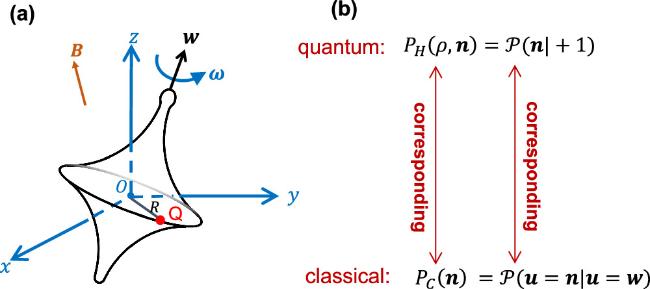
Figure 3. (a) A charged spinning top precessing in a homogeneous magnetic field, which is a classical analogy of a spin-1/2 particle. Here, O is the center-of-mass of the top, and w is the unit vector along the symmetry axis. Other details are introduced in sections |
The above analysis reveals that the charged spinning top is a classical analogy of a quantum spin-1/2 particle. The direction vector w ≡ (wx, wy, wz) of the top axis is just the classical analogy of the Pauli -operator vector $\hat{{\boldsymbol{\sigma }}}\equiv ({\hat{\sigma }}_{x},{\hat{\sigma }}_{y},{\hat{\sigma }}_{z})$ of the spin-1/2 particle. Furthermore, as shown in Appendix B , the classical dynamical equation (13 ) of the top can be re-expressed as a Hamiltonian equation, and the phase space of this system is just the set of all possible direction vectors of the top axis, coinciding with the unit sphere S2. As a result, the state of this classical top is described by the phase-space probability distribution PC(n) with n ∈ S2. Explicitly, PC(n) represents the probability density of the event that the symmetry axis of the top is along n, i.e., w=n.
In the discussion in section 3 , which is for the spin-1/2 quantum particle, we introduced the conditional probability density ${ \mathcal P }\left({\boldsymbol{n}}\left|\right.+1\right)$. Now let us consider the classical correspondence of ${ \mathcal P }\left({\boldsymbol{n}}\left|\right.+1\right)$. As shown above, the classical correspondence of the $\hat{{\boldsymbol{\sigma }}}$-operator is the symmetry axis direction w. Therefore, for a given direction u ∈ S2, the classical correspondence of the event $\hat{{\boldsymbol{\sigma }}}\cdot {\boldsymbol{u}}=+1$ is the event w=u. Therefore, the classical correspondence of ${ \mathcal P }\left({\boldsymbol{n}}\left|\right.+1\right)$ is a conditional probability density ${ \mathcal P }\left({\boldsymbol{u}}={\boldsymbol{n}}\left|\right.{\boldsymbol{w}}={\boldsymbol{u}}\right)$, which is defined as the probability that a random direction u being in a small solid angle ΔΩ around the direction n, under the condition that w=u, is ${ \mathcal P }\left({\boldsymbol{u}}={\boldsymbol{n}}\left|\right.{\boldsymbol{w}}={\boldsymbol{u}}\right){\rm{\Delta }}{\rm{\Omega }}$. Clearly, ${ \mathcal P }\left({\boldsymbol{u}}={\boldsymbol{n}}\left|\right.{\boldsymbol{w}}={\boldsymbol{u}}\right)$ can in principle be measured via a ‘classical version' of the thought experiment in section 3 [12].
Furthermore, for a charged spinning top with phase-space distribution function PC(n), the conditional probability density ${ \mathcal P }\left({\boldsymbol{u}}={\boldsymbol{n}}\left|\right.{\boldsymbol{w}}={\boldsymbol{u}}\right)$ can be calculated via Bayes' theorem as15 ) yields 17 ) into (16 ), and using the normalization condition, we finally obtain
$\begin{eqnarray}{ \mathcal P }\left({\boldsymbol{u}}={\boldsymbol{n}}\left|\right.{\boldsymbol{w}}={\boldsymbol{u}}\right)=\frac{{ \mathcal P }\left({\boldsymbol{w}}={\boldsymbol{u}}\left|\right.{\boldsymbol{u}}={\boldsymbol{n}}\right)}{{ \mathcal P }\left({\boldsymbol{w}}={\boldsymbol{u}}\right)}{ \mathcal P }\left({\boldsymbol{u}}={\boldsymbol{n}}\right),\end{eqnarray}$
where ${ \mathcal P }\left({\boldsymbol{u}}={\boldsymbol{n}}\right)=1/(4\pi )$ is the probability density of the random vector u being n, ${ \mathcal P }\left({\boldsymbol{w}}={\boldsymbol{u}}\left|\right.{\boldsymbol{u}}={\boldsymbol{n}}\right)$ is the probability density of w=u under the condition that u=n, and ${ \mathcal P }\left({\boldsymbol{w}}={\boldsymbol{u}}\right)=\int {\rm{d}}{{\boldsymbol{n}}}^{{\prime} }{ \mathcal P }\left({\boldsymbol{w}}={\boldsymbol{u}}\left|\right.{\boldsymbol{u}}={{\boldsymbol{n}}}^{{\prime} }\right){ \mathcal P }({\boldsymbol{u}}={{\boldsymbol{n}}}^{{\prime} })$. Since ${ \mathcal P }\left({\boldsymbol{u}}={\boldsymbol{n}}\right)$ and ${ \mathcal P }\left({\boldsymbol{w}}={\boldsymbol{u}}\right)$ are all independent of n, equation ( $\begin{eqnarray}{ \mathcal P }\left({\boldsymbol{u}}={\boldsymbol{n}}\left|\right.{\boldsymbol{w}}={\boldsymbol{u}}\right)=\xi { \mathcal P }\left({\boldsymbol{w}}={\boldsymbol{u}}\left|\right.{\boldsymbol{u}}={\boldsymbol{n}}\right),\end{eqnarray}$
where ξ is the normalization factor determined by the condition $\int {\rm{d}}{\boldsymbol{n}}{ \mathcal P }\left({\boldsymbol{u}}={\boldsymbol{n}}\left|\right.{\boldsymbol{w}}={\boldsymbol{u}}\right)=1$. Furthermore, we have $\begin{eqnarray}\begin{array}{rcl}{ \mathcal P }\left({\boldsymbol{w}}={\boldsymbol{u}}\left|\right.{\boldsymbol{u}}={\boldsymbol{n}}\right) & =& { \mathcal P }\left({\boldsymbol{w}}={\boldsymbol{n}}\left|\right.{\boldsymbol{u}}={\boldsymbol{n}}\right)\\ & =& {P}_{C}({\boldsymbol{n}}),\end{array}\end{eqnarray}$
where the second equality is due to the fact that ${ \mathcal P }\left({\boldsymbol{w}}={\boldsymbol{n}}\left|\right.{\boldsymbol{u}}={\boldsymbol{n}}\right)$ is just the probability density of w=n, i.e., PC(n). Substituting equation ( $\begin{eqnarray}{ \mathcal P }\left({\boldsymbol{u}}={\boldsymbol{n}}\left|\right.{\boldsymbol{w}}={\boldsymbol{u}}\right)={P}_{C}({\boldsymbol{n}}).\end{eqnarray}$
As shown above, in our quantum-classical analogy the classical correspondence of ${ \mathcal P }\left({\boldsymbol{n}}\left|\right.+1\right)$ is a conditional probability density ${ \mathcal P }\left({\boldsymbol{u}}={\boldsymbol{n}}\left|\right.{\boldsymbol{w}}={\boldsymbol{u}}\right)$. Additionally, as shown in section 3 , in the quantum case we have ${ \mathcal P }\left({\boldsymbol{n}}\left|\right.+1\right)={P}_{H}(\hat{\rho };{\boldsymbol{n}})$. Moreover, equation (18 ) shows that in the classical side we have ${ \mathcal P }\left({\boldsymbol{u}}={\boldsymbol{n}}\left|\right.{\boldsymbol{w}}={\boldsymbol{u}}\right)={P}_{C}({\boldsymbol{n}})$. Therefore, the classical correspondence of the Husimi function ${P}_{H}(\hat{\rho };{\boldsymbol{n}})$ is the phase-space probability distribution function PC(n) (figure 3(b)).
Using the above conclusion and the relationship between the Wehrl entropy and the Husimi function (i.e., equation (7 )), we further find that the classical analogy of the Wehrl entropy is $-\int {P}_{C}({\boldsymbol{n}})\mathrm{ln}\left[{P}_{C}({\boldsymbol{n}})\right]{\rm{d}}{\boldsymbol{n}}$. This is nothing but the Gibbs entropy of the spinning top because PC(n) is the phase-space probability distribution function of this top.
The above discussions can be directly generalized to the multi-particle cases with N > 1. The classical analogy of N spin-1/2 particles are N charged spinning tops, and the N-body phase space is the product S2⨂N of the N spheres. Similar as above, one can find that the classical analogy of the Husimi function and Wehrl entropy of the N quantum particles are the probability distribution of the tops in this N-body phase space and the corresponding Gibbs entropy, respectively.
5. Continuous-variable systems
The above statistical interoperation of the Husimi function and Wehrl entropy of spin systems can be generalized to the systems with continuous variables. In this section, we illustrate this generalization with the example of a one-dimensional particle moving along the x-axis.
The coherent states of this particle can be denoted as $\{| {\psi }_{{x}_{* },{p}_{* }}\rangle | {x}_{* },{p}_{* }\in {\mathbb{R}}\}$. The real-space wave function of the coherent state $| {\psi }_{{x}_{* },{p}_{* }}\rangle $ is given by
$\begin{eqnarray}\langle x| {\psi }_{{x}_{* },{p}_{* }}\rangle ={\left(\frac{2}{\pi {\sigma }^{2}}\right)}^{\frac{1}{4}}\exp \left[-\frac{{(x-{x}_{* })}^{2}}{{\sigma }^{2}}+\frac{{\rm{i}}{p}_{* }x}{\hslash }\right],\end{eqnarray}$
where ∣x⟩ is the eigenstate of the coordinate operator. Here, σ is an (x*, p*)-independent positive parameter. The state $| {\psi }_{{x}_{* },{p}_{* }}\rangle $ satisfies $\begin{eqnarray}\langle {\psi }_{{x}_{* },{p}_{* }}| \hat{x}| {\psi }_{{x}_{* },{p}_{* }}\rangle ={x}_{* };\langle {\psi }_{{x}_{* },{p}_{* }}| \hat{p}| {\psi }_{{x}_{* },{p}_{* }}\rangle ={p}_{* },\end{eqnarray}$
$\begin{eqnarray}{\rm{\Delta }}x=\frac{\sigma }{2};{\rm{\Delta }}p=\frac{\hslash }{\sigma }=\frac{\frac{1}{2}\hslash }{{\rm{\Delta }}x},\end{eqnarray}$
where $\hat{x}$ and $\hat{p}$ are the coordinate and momentum operators, respectively, and ${\rm{\Delta }}\zeta \equiv {[\langle {\psi }_{{x}_{* },{p}_{* }}| {\hat{\zeta }}^{2}| {\psi }_{{x}_{* },{p}_{* }}\rangle -{\langle {\psi }_{{x}_{* },{p}_{* }}| \hat{\zeta }| {\psi }_{{x}_{* },{p}_{* }}\rangle }^{2}]}^{1/2}$, (ζ=x, p). These results yields that the wave functions of $| {\psi }_{{x}_{* },{p}_{* }}\rangle $ in real and momentum spaces are wave packets centered at x* and p*, respectively, with widths σ/2 and ℏ/σ, respectively.The Husimi function with respect to the density operator $\hat{\rho }$ of this particle is
$\begin{eqnarray}{P}_{H}(\hat{\rho };{x}_{* },{p}_{* })\equiv \frac{1}{2\pi \hslash }\langle {\psi }_{{x}_{* },{p}_{* }}| \hat{\rho }| {\psi }_{{x}_{* },{p}_{* }}\rangle .\end{eqnarray}$
It satisfies the normalization condition $\begin{eqnarray}\int {\rm{d}}{x}_{* }{\rm{d}}{p}_{* }{P}_{H}(\hat{\rho };{x}_{* },{p}_{* })=1.\end{eqnarray}$
The corresponding Wehrl entropy ${S}_{W}(\hat{\rho })$ is defined as $\begin{eqnarray}{S}_{W}(\hat{\rho })\equiv -\int {P}_{H}(\hat{\rho };{x}_{* },{p}_{* })\mathrm{ln}\left[{P}_{H}(\hat{\rho };{x}_{* },{p}_{* })\right]{\rm{d}}{x}_{* }{\rm{d}}{p}_{* }.\end{eqnarray}$
We can obtain a statistical interoperation of ${P}_{H}(\hat{\rho })$ via generalizing the thought experiment of section 4 to the current continuous-variable system. Firstly, we assume there are m copies c(1), c(2), …, c(m) of the particle, with each one being in the same state $\hat{\rho }$. Secondly, the experimenter generates m independent random points $({x}_{* }^{(1)},{p}_{* }^{(1)}),({x}_{* }^{(2)},{p}_{* }^{(2)}),\ldots ,({x}_{* }^{(m)},{p}_{* }^{(m)})$ in the phase space. After that, the experimenter performs the following m steps: in the η-th step (η=1, …, m), the experimenter measures whether the particle is in the coherent state corresponding to $({x}_{* }^{(\eta )},{p}_{* }^{(\eta )})$, i.e., measure the operator $| {\psi }_{{x}_{* }^{(\eta )},{p}_{* }^{(\eta )}}\rangle \langle {\psi }_{{x}_{* }^{(\eta )},{p}_{* }^{(\eta )}}| $ for the copy c(η). The outcome of this measurement is either 0 or 1, since this operator has only these two eigenvalues. If and only if the outcome of this measurement is 1, the experimenter notes down the point $({x}_{* }^{(\eta )},{p}_{* }^{(\eta )})$ in a notebook.
We consider the cases where m is very large. After all these m steps are finished, we can ask: what is the distribution of the points noted down in the notebook? As in section 4 , using the Bayes' theorem one can directly prove that the density distribution of noted points in the phase space is just (up to a normalization constant) the Husimi function ${P}_{H}(\hat{\rho };{x}_{* },{p}_{* })$ with respect to the density operator $\hat{\rho }$ of the particle. Consequently, the corresponding Wehrl entropy ${S}_{W}(\hat{\rho })$ just describes the degree of complexity of this density distribution.
Now, we investigate the classical correspondence of the Husimi function and Wehrl entropy. To this end, as in section 4 , we study the classical analogy of the above thought experiment. We consider a one-dimensional classical particle with coordinate x and momentum p, respectively. The phase-space probability distribution (i.e., the Liouville function) of this particle is ρL(x*, p*). In the thought experiment, the experimenter prepares m copies c(1), c(2), …, c(m) of this particle, and generates an m independent random point $({x}_{* }^{(1)},{p}_{* }^{(1)}),({x}_{* }^{(2)},{p}_{* }^{(2)}),\ldots ,({x}_{* }^{(m)},{p}_{* }^{(m)})$ in the phase space. After that, the experimenter performs the following m steps: in the η-th step (η=1, …, m), the experimenter measures the position and momentum of the copy c(η). If and only if the outcome of this measurement is $x={x}_{* }^{(\eta )}$ and $p={p}_{* }^{(\eta )}$, the experimenter notes down the point $({x}_{* }^{(\eta )},{p}_{* }^{(\eta )})$ in a notebook.
We consider the case where the m steps are very large. After all these steps are completed, the distribution of the points noted down in the notebook is the classical correspondence of the Husimi function PH. On the other hand, with the Bayes' theorem it can be proven that this density distribution is nothing but the Liouville function ρL(x*, p*). Therefore, the classical correspondence of the Husimi function PH is the Liouville function ρ(x*, p*). Accordingly, the classical correspondence of the Wehrl entropy SW is the Gibbs entropy, which is defined as ${S}_{G}=-\int {\rm{d}}{x}_{* }{\rm{d}}{p}_{* }{\rho }_{L}({x}_{* },{p}_{* })\mathrm{ln}\left[{\rho }_{L}({x}_{* },{p}_{* })\right]$ and plays an important role in statistical physics.
6. Summary
In this work we provide a statistical interpretation to the Husimi function and Wehrl entropy for spin-1/2 particles as well as systems with continuous variables, which is based on Bayes' theorem. With this interpretation, we show that the classical correspondence of the Husimi function and Wehrl entropy are just the Liouville function and Gibbs entropy, respectively. This function and entropy are being increasingly utilized in the studies of various quantum systems, and our results are helpful for understanding the properties of these systems.
Acknowledgments
The authors thank Yingfei Gu, Dazhi Xu, Pengfei Zhang, Hui Zhai, Honggang Luo, Zhiyuan Xie, and Ninghua Tong for the fruitful discussions. This work was supported by the National Key Research and Development Program of China [Grant No. 2022YFA1405300 (PZ)], and the Innovation Program for Quantum Science and Technology (Grant No. 2023ZD0300700).
Appendix A Proof of equation (13)
In this appendix, we prove that when the spinning of the top is rapid enough, the unit vector w along the symmetry axis of the top satisfies the dynamical equation (13 ) during the precession.
We first clarify the specific meaning of the above condition ‘spinning of the top is rapid enough'. As shown in figure 4, we denote O-xyz as the center-of-mass (CoM) frame of the top. Without loss of generality, we assume B is along z-direction, i.e., B=B0ez. The angles θ and Φ and polar and azimuthal angles of the direction w of the symmetric axis, respectively. During the motion, the top is spinning around w. In addition, both Φ and θ can also change with time, i.e., there can be precession and nutation. The aforementioned ‘spinning is rapid enough' means that the following two conditions are satisfied simultaneously:
1. $| \omega | \gg | \dot{\phi }| ,| \dot{\theta }| $.
2.The contribution of the precession and nutation to the angular L of the top in the CoM frame is negligible. Namely, L can be approximated as
$\begin{eqnarray}{\boldsymbol{L}}=\omega I{\boldsymbol{w}},\end{eqnarray}$
where I is the corresponding moment of inertia.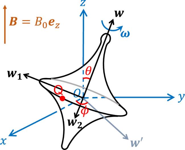
Figure 4. A charged spinning top precessing in a homogeneous magnetic field B=B0ez. Here, O is the CoM of the top, O-xyz is the CoM frame, w is the unit vector along the symmetry axis of the top. The unit vectors w1 and w2 are mutually perpendicular unit vectors, both of which are also perpendicular to w. Other details are introduced in Appendix |
Now we consider the dynamics of the top. According to the angular momentum theorem in the CoM frame, we have A.2 ) with the time-averaged value over a period T=2π/ω: A.3 ) and this approximation, we have
$\begin{eqnarray}\frac{{\rm{d}}{\boldsymbol{L}}}{{\rm{d}}t}={\boldsymbol{M}},\end{eqnarray}$
where M is the instantaneous torque of the Lorentz force on the charge Q in the CoM frame. Due to the above condition (ii), we have $\begin{eqnarray}\frac{{\rm{d}}{\boldsymbol{L}}}{{\rm{d}}t}=I\dot{\omega }{\boldsymbol{w}}+I\omega \frac{{\rm{d}}{\boldsymbol{w}}}{{\rm{d}}t}.\end{eqnarray}$
Furthermore, due to the above condition (i), we can approximately replace the instantaneous torque M in equation ( $\begin{eqnarray}\langle {\boldsymbol{M}}\rangle =\frac{1}{T}{\int }_{0}^{T}{\rm{d}}t{\boldsymbol{M}}(t).\end{eqnarray}$
Using equation ( $\begin{eqnarray}I\dot{\omega }{\boldsymbol{w}}+I\omega \frac{{\rm{d}}{\boldsymbol{w}}}{{\rm{d}}t}=\langle {\boldsymbol{M}}\rangle .\end{eqnarray}$
Now we calculate the average torque ⟨M⟩. To this end, we first notice that the direction vector w can be expressed as
$\begin{eqnarray}{\boldsymbol{w}}=\sin \theta \cos \phi {{\boldsymbol{e}}}_{x}+\sin \theta \sin \phi {{\boldsymbol{e}}}_{y}+\cos \theta {{\boldsymbol{e}}}_{z},\end{eqnarray}$
with ex,y,z being the unit vectors along the x, y, z directions of the CoM frame, respectively. We further introduce unit vectors w1, w2 $\begin{eqnarray}{{\boldsymbol{w}}}_{1}=-\sin \phi {{\boldsymbol{e}}}_{x}+\cos \phi {{\boldsymbol{e}}}_{y},\end{eqnarray}$
$\begin{eqnarray}{{\boldsymbol{w}}}_{2}=-\cos \theta \cos \phi {{\boldsymbol{e}}}_{x}-\cos \theta \sin \phi {{\boldsymbol{e}}}_{y}+\sin \theta {{\boldsymbol{e}}}_{z},\end{eqnarray}$
which are both perpendicular to w, and are perpendicular with each other. The instantaneous torque M(t) is given by $\begin{eqnarray}{\boldsymbol{M}}(t)={{\boldsymbol{F}}}_{{\boldsymbol{L}}}({\boldsymbol{t}})\times {\boldsymbol{r}}({\boldsymbol{t}}),\end{eqnarray}$
where r(t) and FL(t) are the charge position and the Lorentz force, respectively. Explicitly, we have $\begin{eqnarray}{\boldsymbol{r}}({\boldsymbol{t}})=R\cos (\omega t){{\boldsymbol{w}}}_{1}+R\sin (\omega t){{\boldsymbol{w}}}_{2},\end{eqnarray}$
and $\begin{eqnarray}{{\boldsymbol{F}}}_{{\boldsymbol{L}}}({\boldsymbol{t}})=Q{\boldsymbol{v}}({\boldsymbol{t}})\times {\boldsymbol{B}},\end{eqnarray}$
where $\begin{eqnarray}{\boldsymbol{v}}({\boldsymbol{t}})=\frac{{\rm{d}}}{{\rm{d}}t}{\boldsymbol{r}}({\boldsymbol{t}}).\end{eqnarray}$
Using these relations and straightforward calculations, we obtain $\begin{eqnarray}\langle {\boldsymbol{M}}\rangle =\frac{1}{2}Q{R}^{2}\omega {\boldsymbol{w}}\times {\boldsymbol{B}}.\end{eqnarray}$
Substituting equation (A.13 ) into equation (A.5 ), and using the fact that dw/dt⊥w, which is due to the fact that the norm of w does not change with time, we directly obtain equation (13 ) of our main text and $\dot{\omega }=0$.
In the end of this appendix, we point out that the mechanism of the top dynamics shown above is very similar to the one of a rapidly spinning electrically neutral top processing the gravity [13].
Appendix B The phase space of charged spinning top
In this appendix we show that the phase space of the charged spinning top studied in section 4 is just the unit sphere S2.
The canonical coordinate of this top can be chosen as the azimuth angle φ and the z-component wz of the direction vector $\hat{{\boldsymbol{w}}}$ of the top axis (figure 3(a)). Then, the Lagrangian of this system is given by 13 ) of this top, and the x and y components wx,y of the direction vector $\hat{{\boldsymbol{w}}}$ are functions of the canonical coordinates, i.e., ${w}_{x}=\sqrt{1-{w}_{z}^{2}}\cos \varphi $ and ${w}_{y}=\sqrt{1-{w}_{z}^{2}}\sin \varphi $.
$\begin{eqnarray}\begin{array}{rcl}{L}_{{\rm{top}}} & =& C\left[{B}_{z}{w}_{z}+{B}_{x}\sqrt{1-{w}_{z}^{2}}\cos \varphi \right.\\ & & \left.+{B}_{y}\sqrt{1-{w}_{z}^{2}}\sin \varphi \right]+\dot{\varphi }{w}_{z}.\end{array}\end{eqnarray}$
It can be straightforwardly proven that the Lagrangian equations $\begin{eqnarray}\frac{{\rm{d}}}{{\rm{d}}t}\left(\frac{\partial {L}_{{\rm{top}}}}{\partial \dot{\varphi }}\right)-\frac{\partial {L}_{{\rm{top}}}}{\partial \varphi }=0;\end{eqnarray}$
$\begin{eqnarray}\frac{{\rm{d}}}{{\rm{d}}t}\left(\frac{\partial {L}_{{\rm{top}}}}{\partial \dot{{w}_{z}}}\right)-\frac{\partial {L}_{{\rm{top}}}}{\partial {w}_{z}}=0,\end{eqnarray}$
are equivalent to the classical dynamical equation (Moreover, the canonical momentums pφ and pw of our system are canonical coordinates
$\begin{eqnarray}{p}_{\varphi }=\frac{\partial {L}_{{\rm{top}}}}{\partial \dot{\varphi }}={w}_{z};\end{eqnarray}$
$\begin{eqnarray}{p}_{{w}_{z}}=\frac{\partial {L}_{{\rm{top}}}}{\partial \dot{{w}_{z}}}=0.\end{eqnarray}$
Therefore, although there are two canonical coordinates, the phase space of our system is two-dimensional, rather than four-dimensional. Explicitly, this phase space is the space of (φ, wz), with φ ∈ [0, 2π) and wz ∈ [-1, 1]. In addition, the measurement (area element) of this phase space is dφdwz. It is clear that this phase space is equivalent to the unit sphere S2 with azimuth angle being φ and polar angle being $\theta \equiv \arccos {w}_{z}=\arccos {p}_{\varphi }$, i.e., the set of all possible direction vectors $\hat{{\boldsymbol{w}}}$. Moreover, the measurement dφdwz just equals to $\sin \theta {\rm{d}}\theta {\rm{d}}\varphi $, i.e., the area element of the S2 sphere.
Additionally, the Hamiltonian of this charged spinning topB.2 , B.3 ), and thus equivalent to the classical dynamical equation (13 ).
$\begin{eqnarray}\begin{array}{rcl}{H}_{{\rm{top}}} & =& -C\left[{B}_{z}{p}_{\varphi }+{B}_{x}\sqrt{1-{p}_{\varphi }^{2}}\cos \varphi \right.\\ & & \left.+{B}_{y}\sqrt{1-{p}_{\varphi }^{2}}\sin \varphi \right].\end{array}\end{eqnarray}$
The Hamilton equation with respect to Htop is equivalent to the the Lagrangian equations (