


1. Introduction
The long-distance intracellular transports of cargoes such as vesicles, organelles mitochondria, mRNA particles, liposomes, etc, are performed by biological molecular motors that move processively on their linear tracks powered by the chemical energy from ATP hydrolysis [1-4]. Kinesin proteins are a typical group of those molecular motors that can move processively on microtubules (MTs) [5-10]. The dynamics of the cargo transport driven by the molecular motor have been studied both theoretically and experimentally [11-23]. The theoretical studies have been mainly focused on cases where the cargo has no interaction with the track. However, in some cases, the cargo can interact with the track. For example, the kinesin-6 motor, which plays a critical role during the metaphase-anaphase transition and cytokinesis, can transport a major mitotic signaling module, the chromosomal passenger complex (CPC), on the MT track towards the equatorial cortex [24-31]. It was shown that the CPC complex, as the cargo, can interact with the MT [32]. The trafficking kinesin protein 1 (TRAK1 protein), when coupled with the kinesin-1 motor [33-36], can be driven to move towards the MT plus end [37]. The TRAK1 protein, which can interact with the MT [37], can also be regarded as the cargo.
An interesting but unclear issue is how the interaction of the cargo with the track affects the dynamics of the motor transporting the cargo. In this work, we study theoretically the dynamics of the complex of a molecular motor coupled with a cargo (called cargo-motor complex) moving on the track by considering the interaction of the cargo with the track. We firstly present the general theory for the cargo-motor complex. We then apply the theory to the cargo-kinesin-1 and cargo-kinesin-6 complexes.
2. Theory
2.1. Velocity
It is considered that the cargo can interact with the track via, for example, van der Waals force. The detached cargo can bind to the track and the track-bound cargo can detach from the track. After being bound to the track, the single cargo can make the unbiased diffusion along the track, with a diffusion constant D, where D=0 corresponds to the limiting case where the cargo cannot diffuse along the track. The motor can bind to the track and the track-bound motor can detach from the track. After being bound to the track, the single motor can move directionally and processively along the track. It is evident that the movement of the cargo-motor complex on the track can occur during three phases. During the first phase (called Phase I) both the motor and cargo are bound to the track. During the second phase (called Phase II) the cargo is detached and the motor is bound to the track. During the third phase (called Phase III) the motor is detached and the cargo is bound to the track.
We firstly consider the movement during Phase I, when both the motor and cargo are bound to the track (figure 1). In the equilibrium state, where the linker connecting the motor and cargo is neither stretched nor compressed, the distance between the center-of-mass position of the motor and that of the cargo along the track (simply termed as the distance between the motor and cargo) is denoted by l0. Here, we assume that the linker has a large elastic coefficient for stretching and compressing, and thus the magnitude of the change in the distance between the motor and cargo relative to distance l0 is smaller than 2d along the track, with d being the distance between two successive motor-binding (or cargo-binding) sites on the track. In other words, the motor cannot overcome the large energy change of stretching or compressing the linker by a length larger than 2d. For approximation, we consider that when the distance between the motor and cargo is l0 + d the elastic energy change (denoted by ${\rm{\Delta }}E$) has the same value as that when the distance between the motor and cargo is l0 - d (also denoted by ${\rm{\Delta }}E$).
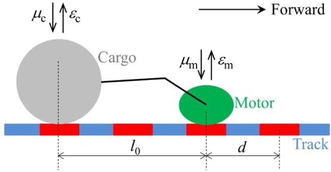
Figure 1. Schematic diagram of the cargo-motor complex. For simplicity, the motor and cargo are modeled as two particles and their detailed structures are not considered. The two successive binding sites of the motor on the track are denoted by d, equal to the period of the structure of the track polymer. The cargo can interact with the track via, for example, van der Waals force. Due to the periodic structure of the track, the interaction potential of the cargo with the track has the periodic form, with the potential period being also equal to that of the track. The motor and cargo are connected by a linker. l0 is the equilibrium distance between the motor and cargo. ${\varepsilon }_{{\rm{m}}}$ is the detachment rate of the motor when the cargo-motor complex is in the equilibrium state with no force on the motor. ${\mu }_{{\rm{m}}}$ is the rebinding rate of the motor when the cargo is bound to the track. ${\varepsilon }_{{\rm{c}}}$ is the detachment rate of the cargo when the cargo-motor complex is in the equilibrium state with no force on the cargo. ${\mu }_{{\rm{c}}}$ is the rebinding rate of the cargo when the motor is bound to the track. |
Consider that the cargo-motor complex is initially in the equilibrium state, which is termed as State A (figure 2). From State A the following four scenarios can occur. (i) From State A, the motor can take a forward step, with the stepping rate denoted by ${k}_{{\rm{m}}}^{(1+)}$, while the cargo is not moved relative to the track. This state, with the distance between the motor and cargo being l0 + d, is termed as State F1 (figure 2). From State F1, either the motor can take a backward step, with the stepping rate denoted by ${k}_{{\rm{m}}}^{(2-)}$, or the cargo can take a forward step, with the stepping rate denoted by ${k}_{{\rm{c}}}^{(2+)}$ (figure 2). From State F1, if the motor takes a backward step, the cargo-motor complex returns to State A, and if the cargo takes a forward step, the cargo-motor complex becomes State F2 (figure 2). In State F2, the cargo-motor complex makes a forward step relative to that in State A. (ii) From State A, the cargo can take a forward step, with the stepping rate denoted by ${k}_{{\rm{c}}}^{(1+)}$, while the motor is not moved relative to the track. This state, with the distance between the motor and cargo being l0 - d, is termed as State F'1 (figure 2). From State F'1, either the cargo can take a backward step, with the stepping rate denoted by ${k}_{{\rm{c}}}^{(2-)}$, or the motor can take a forward step, with the stepping rate denoted by ${k}_{{\rm{m}}}^{(2+)}$ (figure 2). From State F'1, if the cargo takes a backward step, the cargo-motor complex returns to State A, and if the motor takes a forward step, the cargo-motor complex becomes State F2 (figure 2). (iii) From State A, the motor can take a backward step, with the stepping rate denoted by ${k}_{{\rm{m}}}^{(1-)}$, while the cargo is not moved relative to the track. This state, with the distance between the motor and cargo being l0 - d, is termed as State B1 (figure 2). From State B1, either the motor can take a forward step, with the stepping rate denoted by ${k}_{{\rm{m}}}^{(2+)}$, or the cargo can take a backward step, with the stepping rate denoted by ${k}_{{\rm{c}}}^{(2-)}$ (figure 2). From State B1, if the motor takes a forward step the cargo-motor complex returns to State A, and if the cargo takes a backward step the cargo-motor complex becomes State B2 (figure 2). In State B2, the cargo-motor complex makes a backward step relative to that in State A. (iv) From State A, the cargo can take a backward step, with the stepping rate denoted by ${k}_{{\rm{c}}}^{(1-)}$, while the motor is not moved relative to the track. This state, with the distance between the motor and cargo being l0 + d, is termed as State B'1 (figure 2). From State B'1, either the cargo can take a forward step, with the stepping rate denoted by ${k}_{{\rm{c}}}^{(2+)}$, or the motor can take a backward step, with the stepping rate denoted by ${k}_{{\rm{m}}}^{(2-)}$ (figure 2). From State B'1, if the cargo takes a forward step, the cargo-motor complex returns to State A, and if the motor takes a backward step, the cargo-motor complex becomes State B2 (figure 2).
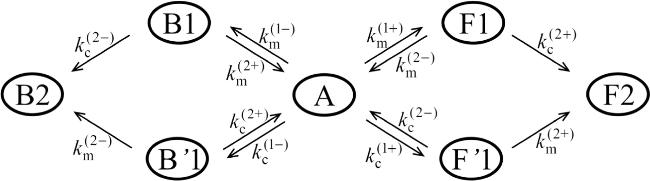
Figure 2. The kinetic pathway of the cargo-motor complex making a forward step and a backward step during Phase I when both the motor and cargo are bound to the track (see text for detailed descriptions). Note that State F2 (State B2) is the same as State A except that the cargo-motor system has made a forward (backward) step in State F2 relative to State A. Thus, the transition from State F2 to State F1, corresponding to a backward step of the cargo relative to the motor, is equivalent to the transition from State A to State B'1. Consequently, the transition from State F2 to State F1 should not be included in the pathway. Similarly, the transition from State F2 to State F'1, the transition from State B2 to State B1 and the transition from State B2 to State B'1 should also not be included. |
Based on the pathway of figure 2, we can derive the following expressions for the rates of the cargo-motor complex taking a forward step and a backward step (see the Supplementary Material):1 ) and (2 ) into the above expression for vI we have
$\begin{eqnarray}{k}_{{\rm{I}}}^{({\rm{Fwd}})}=\displaystyle \frac{\left({k}_{{\rm{m}}}^{(2+)}+{k}_{{\rm{c}}}^{(2-)}\right){k}_{{\rm{m}}}^{(1+)}{k}_{{\rm{c}}}^{(2+)}+\left({k}_{{\rm{c}}}^{(2+)}+{k}_{{\rm{m}}}^{(2-)}\right){k}_{{\rm{c}}}^{(1+)}{k}_{{\rm{m}}}^{(2+)}}{\left({k}_{{\rm{m}}}^{(2+)}+{k}_{{\rm{c}}}^{(2-)}\right)\left({k}_{{\rm{c}}}^{(2+)}+{k}_{{\rm{m}}}^{(2-)}\right)+\left({k}_{{\rm{m}}}^{(1+)}+{k}_{{\rm{c}}}^{(1-)}\right)\left({k}_{{\rm{m}}}^{(2+)}+{k}_{{\rm{c}}}^{(2-)}\right)+\left({k}_{{\rm{c}}}^{(1+)}+{k}_{{\rm{m}}}^{(1-)}\right)\left({k}_{{\rm{c}}}^{(2+)}+{k}_{{\rm{m}}}^{(2-)}\right)},\end{eqnarray}$
$\begin{eqnarray}{k}_{{\rm{I}}}^{({\rm{Bwd}})}=\displaystyle \frac{\left({k}_{{\rm{m}}}^{(2-)}+{k}_{{\rm{c}}}^{(2+)}\right){k}_{{\rm{m}}}^{(1-)}{k}_{{\rm{c}}}^{(2-)}+\left({k}_{{\rm{c}}}^{(2-)}+{k}_{{\rm{m}}}^{(2+)}\right){k}_{{\rm{c}}}^{(1-)}{k}_{{\rm{m}}}^{(2-)}}{\left({k}_{{\rm{m}}}^{(2+)}+{k}_{{\rm{c}}}^{(2-)}\right)\left({k}_{{\rm{c}}}^{(2+)}+{k}_{{\rm{m}}}^{(2-)}\right)+\left({k}_{{\rm{m}}}^{(1+)}+{k}_{{\rm{c}}}^{(1-)}\right)\left({k}_{{\rm{m}}}^{(2+)}+{k}_{{\rm{c}}}^{(2-)}\right)+\left({k}_{{\rm{c}}}^{(1+)}+{k}_{{\rm{m}}}^{(1-)}\right)\left({k}_{{\rm{c}}}^{(2+)}+{k}_{{\rm{m}}}^{(2-)}\right)}.\end{eqnarray}$
The velocity of the cargo-motor complex during Phase I can be written as ${v}_{{\rm{I}}}=\left({k}_{{\rm{I}}}^{({\rm{Fwd}})}-{k}_{{\rm{I}}}^{({\rm{Bwd}})}\right)d$. Substituting equations ( $\begin{eqnarray}{v}_{{\rm{I}}}=\displaystyle \frac{\left({k}_{{\rm{m}}}^{(2+)}+{k}_{{\rm{c}}}^{(2-)}\right)\left({k}_{{\rm{m}}}^{(1+)}{k}_{{\rm{c}}}^{(2+)}-{k}_{{\rm{c}}}^{(1-)}{k}_{{\rm{m}}}^{(2-)}\right)+\left({k}_{{\rm{c}}}^{(2+)}+{k}_{{\rm{m}}}^{(2-)}\right)\left({k}_{{\rm{c}}}^{(1+)}{k}_{{\rm{m}}}^{(2+)}-{k}_{{\rm{m}}}^{(1-)}{k}_{{\rm{c}}}^{(2-)}\right)}{\left({k}_{{\rm{m}}}^{(2+)}+{k}_{{\rm{c}}}^{(2-)}\right)\left({k}_{{\rm{c}}}^{(2+)}+{k}_{{\rm{m}}}^{(2-)}\right)+\left({k}_{{\rm{m}}}^{(1+)}+{k}_{{\rm{c}}}^{(1-)}\right)\left({k}_{{\rm{m}}}^{(2+)}+{k}_{{\rm{c}}}^{(2-)}\right)+\left({k}_{{\rm{c}}}^{(1+)}+{k}_{{\rm{m}}}^{(1-)}\right)\left({k}_{{\rm{c}}}^{(2+)}+{k}_{{\rm{m}}}^{(2-)}\right)}d.\end{eqnarray}$
We secondly consider the movement during Phase II, when the motor is bound to the track while the cargo is detached. The forward and backward stepping rates of the cargo-motor complex can be written as4 ) and (5 ) into the above expression for vII we have
$\begin{eqnarray}{k}_{{\rm{II}}}^{({\rm{Fwd}})}={k}_{{\rm{m}}}^{(0+)},\end{eqnarray}$
$\begin{eqnarray}{k}_{{\rm{II}}}^{({\rm{Bwd}})}={k}_{{\rm{m}}}^{(0-)},\end{eqnarray}$
where ${k}_{{\rm{m}}}^{(0+)}$ and ${k}_{{\rm{m}}}^{(0-)}$ are the respective forward and backward stepping rates of the motor under the condition that there is no external energy change when the motor takes a forward or backward step. The velocity of the cargo-motor complex during Phase II can be written as ${v}_{{\rm{II}}}=\left({k}_{{\rm{II}}}^{({\rm{Fwd}})}-{k}_{{\rm{II}}}^{({\rm{Bwd}})}\right)d$. Substituting equations ( $\begin{eqnarray}{v}_{{\rm{II}}}=\left({k}_{{\rm{m}}}^{(0+)}-{k}_{{\rm{m}}}^{(0-)}\right)d.\end{eqnarray}$
We thirdly consider the movement during Phase III, when the cargo is bound to the track while the motor is detached. The velocity of the cargo-motor complex during Phase III is
$\begin{eqnarray}{v}_{{\rm{III}}}\,=0.\end{eqnarray}$
The stationary probability of the cargo-motor complex in the equilibrium state with the distance between the motor and cargo being l0 can be written as (see the Supplementary Material):
$\begin{eqnarray}{P}_{0}=\displaystyle \frac{\left({k}_{{\rm{m}}}^{(2+)}+{k}_{{\rm{c}}}^{(2-)}\right)\left({k}_{{\rm{c}}}^{(2+)}+{k}_{{\rm{m}}}^{(2-)}\right)}{\left({k}_{{\rm{m}}}^{(2+)}+{k}_{{\rm{c}}}^{(2-)}\right)\left({k}_{{\rm{c}}}^{(2+)}+{k}_{{\rm{m}}}^{(2-)}\right)+\left({k}_{{\rm{m}}}^{(1+)}+{k}_{{\rm{c}}}^{(1-)}\right)\left({k}_{{\rm{m}}}^{(2+)}+{k}_{{\rm{c}}}^{(2-)}\right)+\left({k}_{{\rm{c}}}^{(1+)}+{k}_{{\rm{m}}}^{(1-)}\right)\left({k}_{{\rm{c}}}^{(2+)}+{k}_{{\rm{m}}}^{(2-)}\right)}.\end{eqnarray}$
The stationary probability of the cargo-motor complex in the state with the distance between the motor and cargo being l0 + d can be written as (see the Supplementary Material): $\begin{eqnarray}{P}_{0}^{(+)}=\displaystyle \frac{\left({k}_{{\rm{m}}}^{(1+)}+{k}_{{\rm{c}}}^{(1-)}\right)\left({k}_{{\rm{m}}}^{(2+)}+{k}_{{\rm{c}}}^{(2-)}\right)}{\left({k}_{{\rm{m}}}^{(2+)}+{k}_{{\rm{c}}}^{(2-)}\right)\left({k}_{{\rm{c}}}^{(2+)}+{k}_{{\rm{m}}}^{(2-)}\right)+\left({k}_{{\rm{m}}}^{(1+)}+{k}_{{\rm{c}}}^{(1-)}\right)\left({k}_{{\rm{m}}}^{(2+)}+{k}_{{\rm{c}}}^{(2-)}\right)+\left({k}_{{\rm{c}}}^{(1+)}+{k}_{{\rm{m}}}^{(1-)}\right)\left({k}_{{\rm{c}}}^{(2+)}+{k}_{{\rm{m}}}^{(2-)}\right)}.\end{eqnarray}$
The stationary probability of the cargo-motor complex in the state with the distance between the motor and cargo being l0 - d can be written as (see the Supplementary Material): $\begin{eqnarray}{P}_{0}^{(-)}=\displaystyle \frac{\left({k}_{{\rm{c}}}^{(1+)}+{k}_{{\rm{m}}}^{(1-)}\right)\left({k}_{{\rm{c}}}^{(2+)}+{k}_{{\rm{m}}}^{(2-)}\right)}{\left({k}_{{\rm{m}}}^{(2+)}+{k}_{{\rm{c}}}^{(2-)}\right)\left({k}_{{\rm{c}}}^{(2+)}+{k}_{{\rm{m}}}^{(2-)}\right)+\left({k}_{{\rm{m}}}^{(1+)}+{k}_{{\rm{c}}}^{(1-)}\right)\left({k}_{{\rm{m}}}^{(2+)}+{k}_{{\rm{c}}}^{(2-)}\right)+\left({k}_{{\rm{c}}}^{(1+)}+{k}_{{\rm{m}}}^{(1-)}\right)\left({k}_{{\rm{c}}}^{(2+)}+{k}_{{\rm{m}}}^{(2-)}\right)}.\end{eqnarray}$
We denote by ${\varepsilon }_{{\rm{m}}}$, ${\varepsilon }_{{\rm{m}}}^{(+)}$ and ${\varepsilon }_{{\rm{m}}}^{(-)}$ the detachment rates of the motor when the cargo-motor complex is in the equilibrium state with the distance between the motor and cargo being l0, in the state with the distance between the motor and cargo being l0 + d and in the state with the distance between the motor and cargo being l0 - d, respectively. We denote by ${\mu }_{{\rm{m}}}$ the rebinding rate of the motor when the cargo is bound to the track. We denote by ${\varepsilon }_{{\rm{c}}}$, ${\varepsilon }_{{\rm{c}}}^{(+)}$ and ${\varepsilon }_{{\rm{c}}}^{(-)}$ the detachment rates of the cargo when the cargo-motor complex is in the equilibrium state with the distance between the motor and cargo being l0, in the state with the distance between the motor and cargo being l0 + d and in the state with the distance between the motor and cargo being l0 - d, respectively. We denote by ${\mu }_{{\rm{c}}}$ the rebinding rate of the cargo when the motor is bound to the track. The occurrence probability of Phase II, when the cargo is detached and the motor is bound to the track, can be written as
$\begin{eqnarray}\begin{array}{lll}{P}_{{\rm{II}}} & =& \left({P}_{0}\displaystyle \frac{{\varepsilon }_{{\rm{c}}}}{{\varepsilon }_{{\rm{c}}}+{\mu }_{{\rm{c}}}}+{P}_{0}^{(+)}\displaystyle \frac{{\varepsilon }_{{\rm{c}}}^{(+)}}{{\varepsilon }_{{\rm{c}}}^{(+)}+{\mu }_{{\rm{c}}}}\right.\\ & & \left.+{P}_{0}^{(-)}\displaystyle \frac{{\varepsilon }_{{\rm{c}}}^{(-)}}{{\varepsilon }_{{\rm{c}}}^{(-)}+{\mu }_{{\rm{c}}}}\right)\left[1-\left({P}_{0}\displaystyle \frac{{\varepsilon }_{{\rm{m}}}}{{\varepsilon }_{{\rm{m}}}+{\mu }_{{\rm{m}}}}\right.\right.\\ & & \left.\left.+{P}_{0}^{(+)}\displaystyle \frac{{\varepsilon }_{{\rm{m}}}^{(+)}}{{\varepsilon }_{{\rm{m}}}^{(+)}+{\mu }_{{\rm{m}}}}+{P}_{0}^{(-)}\displaystyle \frac{{\varepsilon }_{{\rm{m}}}^{(-)}}{{\varepsilon }_{{\rm{m}}}^{(-)}+{\mu }_{{\rm{m}}}}\right)\right].\end{array}\end{eqnarray}$
The occurrence probability of Phase III, when the motor is detached and the cargo is bound to the track, can be written as $\begin{eqnarray}\begin{array}{lll}{P}_{{\rm{III}}} & =& \left({P}_{0}\displaystyle \frac{{\varepsilon }_{{\rm{m}}}}{{\varepsilon }_{{\rm{m}}}+{\mu }_{{\rm{m}}}}+{P}_{0}^{(+)}\displaystyle \frac{{\varepsilon }_{{\rm{m}}}^{(+)}}{{\varepsilon }_{{\rm{m}}}^{(+)}+{\mu }_{{\rm{m}}}}\right.\\ & & \left.+{P}_{0}^{(-)}\displaystyle \frac{{\varepsilon }_{{\rm{m}}}^{(-)}}{{\varepsilon }_{{\rm{m}}}^{(-)}+{\mu }_{{\rm{m}}}}\right)\left[1-\left({P}_{0}\displaystyle \frac{{\varepsilon }_{{\rm{c}}}}{{\varepsilon }_{c}+{\mu }_{{\rm{c}}}}\right.\right.\\ & & \left.\left.+{P}_{0}^{(+)}\displaystyle \frac{{\varepsilon }_{{\rm{c}}}^{(+)}}{{\varepsilon }_{{\rm{c}}}^{(+)}+{\mu }_{{\rm{c}}}}+{P}_{0}^{(-)}\displaystyle \frac{{\varepsilon }_{{\rm{c}}}^{(-)}}{{\varepsilon }_{{\rm{c}}}^{(-)}+{\mu }_{{\rm{c}}}}\right)\right].\end{array}\end{eqnarray}$
Thus, the occurrence probability of Phase I, when both the motor and cargo are bound to the track, can be written as $\begin{eqnarray}\begin{array}{rcl}{P}_{{\rm{I}}} & =& 1-{P}_{\mathrm{II}}-{P}_{\mathrm{III}}-\left({P}_{0}\displaystyle \frac{{\varepsilon }_{{\rm{m}}}}{{\varepsilon }_{{\rm{m}}}+{\mu }_{{\rm{m}}}}+{P}_{0}^{(+)}\displaystyle \frac{{\varepsilon }_{{\rm{m}}}^{(+)}}{{\varepsilon }_{{\rm{m}}}^{(+)}+{\mu }_{{\rm{m}}}}\right.\\ & & \left.+\,{P}_{0}^{(-)}\displaystyle \frac{{\varepsilon }_{{\rm{m}}}^{(-)}}{{\varepsilon }_{{\rm{m}}}^{(-)}+{\mu }_{{\rm{m}}}}\right)\left({P}_{0}\displaystyle \frac{{\varepsilon }_{{\rm{c}}}}{{\varepsilon }_{{\rm{c}}}+{\mu }_{{\rm{c}}}}\right.\\ & & \left.+\,{P}_{0}^{(+)}\displaystyle \frac{{\varepsilon }_{{\rm{c}}}^{(+)}}{{\varepsilon }_{{\rm{c}}}^{(+)}+{\mu }_{{\rm{c}}}}+{P}_{0}^{(-)}\displaystyle \frac{{\varepsilon }_{{\rm{c}}}^{(-)}}{{\varepsilon }_{{\rm{c}}}^{(-)}+{\mu }_{{\rm{c}}}}\right),\end{array}\end{eqnarray}$
where the fourth term on the right-hand side represents the occurrence probability when both the motor and cargo are detached.Taken together, the overall velocity of the cargo-motor complex can be written as
$\begin{eqnarray}v=\displaystyle \frac{{P}_{{\rm{I}}}{v}_{{\rm{I}}}+{P}_{{\rm{II}}}{v}_{{\rm{II}}}+{P}_{{\rm{III}}}{v}_{{\rm{III}}}}{{P}_{{\rm{I}}}+{P}_{{\rm{II}}}+{P}_{{\rm{III}}}}.\end{eqnarray}$
Now, we present the expressions for the stepping rates of the motor, ${k}_{{\rm{m}}}^{(0+)}$, ${k}_{{\rm{m}}}^{(0-)}$, ${k}_{{\rm{m}}}^{(1+)}$, ${k}_{{\rm{m}}}^{(1-)}$, ${k}_{{\rm{m}}}^{(2+)}$ and ${k}_{{\rm{m}}}^{(2-)}$, and the stepping rate of the cargo, ${k}_{{\rm{c}}}^{(1+)}$, ${k}_{{\rm{c}}}^{(1-)}$, ${k}_{{\rm{c}}}^{(2+)}$ and ${k}_{{\rm{c}}}^{(2-)}$. For the motor, we take kinesin as an example. As determined before [38], the stepping rates ${k}_{{\rm{m}}}^{(0+)}$, ${k}_{{\rm{m}}}^{(0-)}$, ${k}_{{\rm{m}}}^{(1+)}$, ${k}_{{\rm{m}}}^{(1-)}$, ${k}_{{\rm{m}}}^{(2+)}$ and ${k}_{{\rm{m}}}^{(2-)}$ can be written as $\begin{eqnarray}{k}_{{\rm{m}}}^{(0+)}=\displaystyle \frac{\exp \left(\beta {E}_{0}\right)}{\exp \left(\beta {E}_{0}\right)+1}{k}^{(+)},\end{eqnarray}$
$\begin{eqnarray}{k}_{{\rm{m}}}^{(0-)}=\displaystyle \frac{1}{\exp \left(\beta {E}_{0}\right)+1}{k}^{(-)},\end{eqnarray}$
$\begin{eqnarray}{k}_{{\rm{m}}}^{(1+)}=\displaystyle \frac{\exp \left(\beta {E}_{0}-\beta {\lambda }_{{\rm{m}}}{\rm{\Delta }}E\right)}{\exp \left(\beta {E}_{0}-\beta {\lambda }_{{\rm{m}}}{\rm{\Delta }}E\right)+1}{k}^{(+)},\end{eqnarray}$
$\begin{eqnarray}{k}_{{\rm{m}}}^{(1-)}=\displaystyle \frac{1}{\exp \left(\beta {E}_{0}-\beta {\lambda }_{{\rm{m}}}{\rm{\Delta }}E\right)+1}{k}^{(-)},\end{eqnarray}$
$\begin{eqnarray}{k}_{{\rm{m}}}^{(2+)}=\displaystyle \frac{\exp \left(\beta {E}_{0}+\beta {\lambda }_{{\rm{m}}}{\rm{\Delta }}E\right)}{\exp \left(\beta {E}_{0}+\beta {\lambda }_{{\rm{m}}}{\rm{\Delta }}E\right)+1}{k}^{(+)},\end{eqnarray}$
$\begin{eqnarray}{k}_{{\rm{m}}}^{(2-)}=\displaystyle \frac{1}{\exp \left(\beta {E}_{0}+\beta {\lambda }_{{\rm{m}}}{\rm{\Delta }}E\right)+1}{k}^{(-)},\end{eqnarray}$
where ${\beta }^{-1}={k}_{{\rm{B}}}T$ is the Boltzmann constant times the absolute temperature, E0 is the free energy change associated with the large conformational change and neck-linker docking of the kinesin head induced by ATP binding, which is equivalent to an internal energy of the motor gained from the consumption of an ATP to facilitate its forward movement, k(+) is the ATPase rate of the trailing head, k(-) is the ATPase rate of the leading head, and ${\lambda }_{{\rm{m}}}$ is the splitting factor for the energy change ${\rm{\Delta }}E$ of the system when the motor takes a step relative to the cargo.In general, it is considered that the cargo can make an unbiased diffusion along the track, with the diffusion constant D. At the limiting case that the cargo cannot diffuse on the track, D=0. Under the condition that there is no energy change when the cargo takes a forward or backward step, the relationship between the forward or backward stepping rate and diffusion constant D of the cargo has the form
$\begin{eqnarray}D={k}_{{\rm{c}}}^{(0)}{d}^{2},\end{eqnarray}$
where ${k}_{{\rm{c}}}^{(0)}$ is the forward or backward stepping rate. With ${k}_{{\rm{c}}}^{(0)}$, the rates ${k}_{{\rm{c}}}^{(1+)}$, ${k}_{{\rm{c}}}^{(1-)}$, ${k}_{{\rm{c}}}^{(2+)}$ and ${k}_{{\rm{c}}}^{(2-)}$ can be written as [39,40] $\begin{eqnarray}{k}_{{\rm{c}}}^{(1+)}={k}_{{\rm{c}}}^{(0)}\exp \left(-{\lambda }_{{\rm{c}}}\beta {\rm{\Delta }}E\right),\end{eqnarray}$
$\begin{eqnarray}{k}_{{\rm{c}}}^{(1-)}={k}_{{\rm{c}}}^{(0)}\exp \left[-\left(1-{\lambda }_{{\rm{c}}}\right)\beta {\rm{\Delta }}E\right],\end{eqnarray}$
$\begin{eqnarray}{k}_{{\rm{c}}}^{(2+)}={k}_{{\rm{c}}}^{(0)}\exp \left({\lambda }_{{\rm{c}}}\beta {\rm{\Delta }}E\right),\end{eqnarray}$
$\begin{eqnarray}{k}_{{\rm{c}}}^{(2-)}={k}_{{\rm{c}}}^{(0)}\exp \left[\left(1-{\lambda }_{{\rm{c}}}\right)\beta {\rm{\Delta }}E\right],\end{eqnarray}$
where ${\lambda }_{{\rm{c}}}$ is the splitting factor for the energy change ${\rm{\Delta }}E$ when the cargo takes a step relative to the motor.The detachment rates ${\varepsilon }_{{\rm{m}}}^{(+)}$ and ${\varepsilon }_{{\rm{m}}}^{(-)}$ of the motor can be approximately written as
$\begin{eqnarray}{\varepsilon }_{{\rm{m}}}^{(+)}={\varepsilon }_{{\rm{m}}}\exp \left(\beta {\lambda }_{{\rm{m}}}^{(+)}{\rm{\Delta }}E\right),\end{eqnarray}$
$\begin{eqnarray}{\varepsilon }_{{\rm{m}}}^{(-)}={\varepsilon }_{{\rm{m}}}\exp \left(\beta {\lambda }_{{\rm{m}}}^{(-)}{\rm{\Delta }}E\right),\end{eqnarray}$
where ${\lambda }_{{\rm{m}}}^{(+)}$ and ${\lambda }_{{\rm{m}}}^{(-)}$ are constants. The detachment rates ${\varepsilon }_{{\rm{c}}}^{(+)}$ and ${\varepsilon }_{{\rm{c}}}^{(-)}$ of the cargo can be written as $\begin{eqnarray}{\varepsilon }_{{\rm{c}}}^{(+)}={\varepsilon }_{{\rm{c}}}\exp \left(\beta {\lambda }_{{\rm{c}}}^{(+)}{\rm{\Delta }}E\right),\end{eqnarray}$
$\begin{eqnarray}{\varepsilon }_{{\rm{c}}}^{(-)}={\varepsilon }_{{\rm{c}}}\exp \left(\beta {\lambda }_{{\rm{c}}}^{(-)}{\rm{\Delta }}E\right),\end{eqnarray}$
where ${\lambda }_{{\rm{c}}}^{(+)}$ and ${\lambda }_{{\rm{c}}}^{(-)}$ are constants.It is noted that if the motor is replaced with a protein that can make the unbiased diffusion along the track, that is, if rates ${k}_{{\rm{m}}}^{(0+)}$, ${k}_{{\rm{m}}}^{(0-)}$, ${k}_{{\rm{m}}}^{(1+)}$, ${k}_{{\rm{m}}}^{(1-)}$, ${k}_{{\rm{m}}}^{(2+)}$ and ${k}_{{\rm{m}}}^{(2-)}$ described by equations (15 )-(30 ) are replaced by ${k}_{{\rm{m}}}^{(0+)}={k}_{{\rm{m}}}^{(0-)}={k}_{{\rm{m}}}^{(0)}$, ${k}_{{\rm{m}}}^{(1+)}={k}_{{\rm{m}}}^{(0)}\exp \left(-{\lambda }_{{\rm{m}}}\beta {\rm{\Delta }}E\right)$, ${k}_{{\rm{m}}}^{(1-)}={k}_{{\rm{m}}}^{(0)}\exp \left[-\left(1-{\lambda }_{{\rm{m}}}\right)\beta {\rm{\Delta }}E\right]$, ${k}_{{\rm{m}}}^{(2+)}={k}_{{\rm{m}}}^{(0)}\exp \left({\lambda }_{{\rm{m}}}\beta {\rm{\Delta }}E\right)$ and ${k}_{{\rm{m}}}^{(2-)}={k}_{{\rm{m}}}^{(0)}\exp \left[\left(1-{\lambda }_{{\rm{m}}}\right)\beta {\rm{\Delta }}E\right]$, which are analogous to equations (21 )-(25 ), from equations (3 ), (6 ) and (7 ) we see that ${v}_{{\rm{I}}}$=0, ${v}_{{\rm{II}}}$=0 and ${v}_{{\rm{III}}}$=0. Thus, from equation (14 ) we have v=0. This is consistent with our expectation that the complex of two coupled unbiasedly-diffusive Brownian particles also diffuses unbiasedly.
2.2. Run length
It is noted that the detachment of the cargo-motor complex from the track can occur mainly via two scenarios. The first scenario (called Scenario I') is that the cargo detaches first and then the motor detaches. The second scenario (called Scenario II') is that the motor detaches first and then the cargo detaches.
We first consider Scenario I'. If, before the detachment of the cargo, the complex is in the state with the distance between the motor and cargo being l0, l0 + d and l0 - d, the occurrence probability of the phase when the motor is bound to the track and the cargo is detached has the form of ${\varepsilon }_{{\rm{c}}}/\left({\varepsilon }_{{\rm{c}}}+{\mu }_{{\rm{c}}}\right)$, ${\varepsilon }_{{\rm{c}}}^{(+)}/\left({\varepsilon }_{{\rm{c}}}^{(+)}+{\mu }_{{\rm{c}}}\right)$ and ${\varepsilon }_{{\rm{c}}}^{(-)}/\left({\varepsilon }_{{\rm{c}}}^{(-)}+{\mu }_{{\rm{c}}}\right)$, respectively. Thus, the detachment rate of the cargo-motor complex via Scenario I' can be written as
$\begin{eqnarray}\begin{array}{lll}{\varepsilon }_{{\rm{I}}} & =& {P}_{0}\displaystyle \frac{{\varepsilon }_{{\rm{c}}}\displaystyle \frac{{\varepsilon }_{{\rm{c}}}}{{\varepsilon }_{{\rm{c}}}+{\mu }_{{\rm{c}}}}{\varepsilon }_{{\rm{m}}}}{{\varepsilon }_{{\rm{c}}}+\displaystyle \frac{{\varepsilon }_{{\rm{c}}}}{{\varepsilon }_{{\rm{c}}}+{\mu }_{{\rm{c}}}}{\varepsilon }_{{\rm{m}}}}+{P}_{0}^{(+)}\displaystyle \frac{{\varepsilon }_{{\rm{c}}}^{(+)}\displaystyle \frac{{\varepsilon }_{{\rm{c}}}^{(+)}}{{\varepsilon }_{{\rm{c}}}^{(+)}+{\mu }_{{\rm{c}}}}{\varepsilon }_{{\rm{m}}}}{{\varepsilon }_{{\rm{c}}}^{(+)}+\displaystyle \frac{{\varepsilon }_{{\rm{c}}}^{(+)}}{{\varepsilon }_{{\rm{c}}}^{(+)}+{\mu }_{{\rm{c}}}}{\varepsilon }_{{\rm{m}}}}\\ & & +{P}_{0}^{(-)}\displaystyle \frac{{\varepsilon }_{{\rm{c}}}^{(-)}\displaystyle \frac{{\varepsilon }_{{\rm{c}}}^{(-)}}{{\varepsilon }_{{\rm{c}}}^{(-)}+{\mu }_{{\rm{c}}}}{\varepsilon }_{{\rm{m}}}}{{\varepsilon }_{{\rm{c}}}^{(-)}+\displaystyle \frac{{\varepsilon }_{{\rm{c}}}^{(-)}}{{\varepsilon }_{{\rm{c}}}^{(-)}+{\mu }_{{\rm{c}}}}{\varepsilon }_{{\rm{m}}}}.\end{array}\end{eqnarray}$
The occurrence probability of Scenario I' can be written as $\begin{eqnarray}P{\mbox{'}}_{{\rm{I}}}={P}_{0}\displaystyle \frac{{\varepsilon }_{{\rm{c}}}}{{\varepsilon }_{{\rm{c}}}+{\varepsilon }_{{\rm{m}}}}+{P}_{0}^{(+)}\displaystyle \frac{{\varepsilon }_{{\rm{c}}}^{(+)}}{{\varepsilon }_{{\rm{c}}}^{(+)}+{\varepsilon }_{{\rm{m}}}^{(+)}}+{P}_{0}^{(-)}\displaystyle \frac{{\varepsilon }_{{\rm{c}}}^{(-)}}{{\varepsilon }_{{\rm{c}}}^{(-)}+{\varepsilon }_{{\rm{m}}}^{(-)}}.\end{eqnarray}$
We then consider Scenario II'. If, before the detachment of the motor, the complex is in the state with the distance between the motor and cargo being l0, l0 + d and l0 - d, the occurrence probability of the phase when the cargo is bound to the track and the motor is detached has the form of ${\varepsilon }_{{\rm{m}}}/\left({\varepsilon }_{{\rm{m}}}+{\mu }_{{\rm{m}}}\right)$, ${\varepsilon }_{{\rm{m}}}^{(+)}/\left({\varepsilon }_{{\rm{m}}}^{(+)}+{\mu }_{{\rm{m}}}\right)$ and ${\varepsilon }_{{\rm{m}}}^{(-)}/\left({\varepsilon }_{{\rm{m}}}^{(-)}+{\mu }_{{\rm{m}}}\right)$, respectively. Thus, the detachment rate of the cargo-motor complex via Scenario II' can be written as
$\begin{eqnarray}\begin{array}{lll}{\varepsilon }_{{\rm{II}}} & =& {P}_{0}\displaystyle \frac{{\varepsilon }_{{\rm{m}}}\displaystyle \frac{{\varepsilon }_{{\rm{m}}}}{{\varepsilon }_{{\rm{m}}}+{\mu }_{{\rm{m}}}}{\varepsilon }_{{\rm{c}}}}{{\varepsilon }_{{\rm{m}}}+\displaystyle \frac{{\varepsilon }_{{\rm{m}}}}{{\varepsilon }_{{\rm{m}}}+{\mu }_{{\rm{m}}}}{\varepsilon }_{{\rm{c}}}}+{P}_{0}^{(+)}\displaystyle \frac{{\varepsilon }_{{\rm{m}}}^{(+)}\displaystyle \frac{{\varepsilon }_{{\rm{m}}}^{(+)}}{{\varepsilon }_{{\rm{m}}}^{(+)}+{\mu }_{{\rm{m}}}}{\varepsilon }_{{\rm{c}}}}{{\varepsilon }_{{\rm{m}}}^{(+)}+\displaystyle \frac{{\varepsilon }_{{\rm{m}}}^{(+)}}{{\varepsilon }_{{\rm{m}}}^{(+)}+{\mu }_{{\rm{m}}}}{\varepsilon }_{{\rm{c}}}}\\ & & +{P}_{0}^{(-)}\displaystyle \frac{{\varepsilon }_{{\rm{m}}}^{(-)}\displaystyle \frac{{\varepsilon }_{{\rm{m}}}^{(-)}}{{\varepsilon }_{{\rm{m}}}^{(-)}+{\mu }_{{\rm{m}}}}{\varepsilon }_{{\rm{c}}}}{{\varepsilon }_{{\rm{m}}}^{(-)}+\displaystyle \frac{{\varepsilon }_{{\rm{m}}}^{(-)}}{{\varepsilon }_{{\rm{m}}}^{(-)}+{\mu }_{{\rm{m}}}}{\varepsilon }_{{\rm{c}}}}.\end{array}\end{eqnarray}$
The occurrence probability of Scenario II' can be written as $\begin{eqnarray}P{\mbox{'}}_{{\rm{II}}}={P}_{0}\displaystyle \frac{{\varepsilon }_{{\rm{m}}}}{{\varepsilon }_{{\rm{m}}}+{\varepsilon }_{{\rm{c}}}}+{P}_{0}^{(+)}\displaystyle \frac{{\varepsilon }_{{\rm{m}}}^{(+)}}{{\varepsilon }_{{\rm{m}}}^{(+)}+{\varepsilon }_{{\rm{c}}}^{(+)}}+{P}_{0}^{(-)}\displaystyle \frac{{\varepsilon }_{{\rm{m}}}^{(-)}}{{\varepsilon }_{{\rm{m}}}^{(-)}+{\varepsilon }_{{\rm{c}}}^{(-)}}.\end{eqnarray}$
Taken together, the overall detachment rate of the cargo-motor complex can be calculated by $\begin{eqnarray}\varepsilon =P{\mbox{'}}_{{\rm{I}}}{\varepsilon }_{{\rm{I}}}+P{\mbox{'}}_{{\rm{II}}}{\varepsilon }_{{\rm{II}}}.\end{eqnarray}$
The run length of the cargo-motor complex can be calculated by $\begin{eqnarray}L=\displaystyle \frac{v}{\varepsilon }.\end{eqnarray}$
3. Application of the general theory to cargo-kinesin-1 and cargo-kinesin-6 complexes
In this section, we use the equations presented in the above section to study the velocity and run length of the cargo-kinesin-1 and cargo-kinesin-6 complexes on MTs, with d=8 nm. In the calculation, we take ${\rm{\Delta }}\varepsilon $=6kBT. The parameter values for the kinesin-1 motor, kinesin-6 motor and cargo are chosen as follows.
As determined before [38], with E0=3.5kBT, k(+)=97 ${{\rm{s}}}^{-1}$, k(-)=3 ${{\rm{s}}}^{-1}$ and ${\lambda }_{{\rm{m}}}$=0.43, the theoretical results reproduced quantitatively the available single molecule optical trapping data on the dependence of velocity upon load for Drosophila kinesin-1 motor [11]. Thus, we take E0=3.5kBT, k(+)=97 ${{\rm{s}}}^{-1}$, k(-)=3 ${{\rm{s}}}^{-1}$ and ${\lambda }_{{\rm{m}}}$=0.43 for the kinesin-1 motor (table 1). To be consistent with the available experimental data [11], we take ${\varepsilon }_{{\rm{m}}}$=1 ${{\rm{s}}}^{-1}$ (table 1). As done before [41-45], we take ${\mu }_{{\rm{m}}}$=5 ${{\rm{s}}}^{-1}$ (table 1). As shown before [46], the single molecule optical trapping data on the dependence of the detachment rate of the kinesin-1 motor upon backward load F can be approximately fit to the function ${\varepsilon }_{{\rm{m}}}^{(+)}={\varepsilon }_{{\rm{m}}}\exp \left(\left|F\right|/{F}_{{\rm{d}}}^{(+)}\right)$, with ${F}_{{\rm{d}}}^{(+)}$ $\approx $ 4 pN. From this function and equation (26 ), we have the equation, $\beta {\lambda }_{{\rm{m}}}^{(+)}{\rm{\Delta }}\varepsilon =F/{F}_{{\rm{d}}}^{(+)}$. Approximating the linker as a linear spring, we have the equation, $F=2{\rm{\Delta }}\varepsilon /d$. From the above two equations, we obtain ${\lambda }_{{\rm{m}}}^{(+)}=2/\left(d\beta {F}_{{\rm{d}}}^{(+)}\right)\approx 0.25$. Thus, here we take ${\lambda }_{{\rm{m}}}^{(+)}$=0.25 (table 1). The detachment rate versus forward load F can be approximately calculated by ${\varepsilon }_{{\rm{m}}}^{(-)}={\varepsilon }_{{\rm{m}}}\exp \left(\left|F\right|/{F}_{{\rm{d}}}^{(-)}\right)$, with ${F}_{{\rm{d}}}^{(-)}={F}_{{\rm{d}}}^{(+)}/3$ [45]. Thus, we take ${\lambda }_{{\rm{m}}}^{(-)}$=$3{\lambda }_{{\rm{m}}}^{(+)}$ (table 1).
Table 1. Values of parameters used in the calculation for kinesin-1 and kinesin-6 motors. E0 is the free energy change associated with the large conformational change and neck-linker docking of the kinesin head induced by ATP binding, k(+) is the ATPase rate of the trailing head, k(-) is the ATPase rate of the leading head, ${\lambda }_{{\rm{m}}}$ is the splitting factor for the energy change of the system when the motor takes a step relative to the cargo, ${\varepsilon }_{{\rm{m}}}$ is the detachment rate of the motor when the cargo-motor complex is in the equilibrium state with no force on the motor, ${\mu }_{{\rm{m}}}$ is the rebinding rate of the motor when the cargo is bound to the track, and ${\lambda }_{{\rm{m}}}^{(+)}$ and ${\lambda }_{{\rm{m}}}^{(-)}$ are force-sensitivity parameters for the detachment of the motor under forward and backward forces, respectively. The sources of the parameter values are described in section |
| Parameter | kinesin-1 | kinesin-6 |
|---|---|---|
| E0 (kBT) | 3.5 | 1.75 |
| k(+) (${{\rm{s}}}^{-1}$) | 97 | 97 |
| k(-) (${{\rm{s}}}^{-1}$) | 3 | 3 |
| ${\lambda }_{{\rm{m}}}$ | 0.43 | 0.43 |
| ${\varepsilon }_{{\rm{m}}}$ (${{\rm{s}}}^{-1}$) | 1 | 1 |
| ${\mu }_{{\rm{m}}}$ (${{\rm{s}}}^{-1}$) | 5 | 5 |
| ${\lambda }_{{\rm{m}}}^{(+)}$ | 0.25 | 0.25 |
| ${\lambda }_{{\rm{m}}}^{(-)}$ | $3{\lambda }_{{\rm{m}}}^{(+)}$ | $3{\lambda }_{{\rm{m}}}^{(+)}$ |
The available structural data for the kinesin-6 MKLP2 motor indicated that although the ATP-head has a large conformational change compared to the nucleotide-free head, no neck-linker docking occurs in the ATP-head [47]. As done before [48], assuming that the free energy change of the large conformational change of the ATP-head has a similar value to that of the neck-linker docking, the value of E0 for the kinesin-6 is about half of that for the kinesin-1. Thus, for the kinesin-6, we take E0=1.75kBT (table 1) and for simplicity all other parameter values are the same as those for the kinesin-1 (table 1).
For the cargo, we take ${\lambda }_{{\rm{c}}}$=0.5, as usually done in the literature for the MT-associated proteins that can make the unbiased diffusion on MTs [39,40]. Similar to ${\lambda }_{{\rm{m}}}^{(+)}$, we take ${\lambda }_{{\rm{c}}}^{(+)}$=${\lambda }_{{\rm{c}}}^{(-)}$=0.25. Note that the velocity v and run length L of the cargo-motor complex are insensitive to the variation of ${\lambda }_{{\rm{c}}}^{(+)}$ and ${\lambda }_{{\rm{c}}}^{(-)}$ (see figures S1 and S2 in the Supplementary Material). We take the D, ${\varepsilon }_{{\rm{c}}}$ and ${\mu }_{{\rm{c}}}$ to be variable, where D is the diffusion constant of the single cargo, ${\varepsilon }_{{\rm{c}}}$ is the detachment rate of the cargo when the cargo-motor complex is in the equilibrium state with no force on the cargo and ${\mu }_{{\rm{c}}}$ is the rebinding rate of the cargo when the motor is bound to the track (see above).
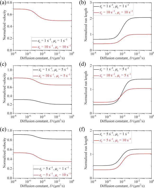
First, we present the results for the cargo-kinesin-1 complex. In figure 3 we show the normalized velocity and run length versus D for different values of ${\varepsilon }_{{\rm{c}}}$ and ${\mu }_{{\rm{c}}}$ (with some results for the occurrence probabilities of Phase I, Phase II and Phase III as well as the occurrence probabilities of Scenario I' and Scenario II' being shown in figure S3 in the Supplementary Material). The normalized velocity and run length are defined as the ratio of the velocity v calculated by equation (14 ) and run length L calculated by equation (35 ) for the case where the cargo has an interaction with the MT track to the velocity vII calculated by equation (6 ) and run length calculated by ${v}_{{\rm{II}}}/{\varepsilon }_{{\rm{m}}}$ for the case where the cargo has no interaction with the MT track. From figure 3, it is seen that when D $\geqslant $ 0.1 μm2 s-1, the velocity can be slightly or evidently larger than that when D is small. More interestingly, it is seen that when D $\geqslant $ 0.1 μm2 s-1, the run length is evidently larger than that when D is small and is larger than that when the cargo has no interaction with the track. In figure 4, we show the normalized velocity and run length versus ${\mu }_{{\rm{c}}}$ for different values of ${\varepsilon }_{{\rm{c}}}$ and D=0.1 μm2 s-1. It is seen that as ${\mu }_{{\rm{c}}}$ increases, the velocity decreases and the run length increases. In figure 5, we show the normalized velocity and run length versus ${\varepsilon }_{{\rm{c}}}$ for different values of ${\mu }_{{\rm{c}}}$ and D=0.1 μm2 s-1. It is seen that as ${\varepsilon }_{{\rm{c}}}$ increases, the velocity increases and the run length decreases significantly. Interestingly, it is noted that at ${\mu }_{{\rm{c}}}$=10 ${{\rm{s}}}^{-1}$ and ${\varepsilon }_{{\rm{c}}}$=1.75 ${{\rm{s}}}^{-1}$, the normalized velocity and run length are in quantitative agreement with prior experimental data for the TRAK1-kinesin-1 complex [37]. Note that in the experiment, Rattus norvegicus kinesin-1 was used [37]. Since the parameter values for the Rattus norvegicus kinesin-1 are not unknown and the parameter values for the Drosophila kinesin-1 motor were determined before [11], for simplicity, in figure 5 we take the Rattus norvegicus kinesin-1 having the same parameter values as the Drosophila kinesin-1. In fact, by taking k(+)=118.3 ${{\rm{s}}}^{-1}$, ${\varepsilon }_{{\rm{m}}}$= 0.596 ${{\rm{s}}}^{-1}$ and ${\mu }_{{\rm{m}}}$= 3.3 ${{\rm{s}}}^{-1}$ while other parameter values to be the same as those used to obtain the red lines in figure 5, the experimentally measured velocity of 918 nm s-1 and run length of 1.54 μm for the Rattus norvegicus kinesin-1 alone can be reproduced theoretically, and the experimental velocity and run length for the TRAK1-kinesin-1 complex can also be explained well [37] (figures S4(a) and (b) in the Supplementary Material). Moreover, it is predicted that for the TRAK1-kinesin-1 complex Phase I with both the motor and cargo bound to the track is more favored and Scenario I' with the cargo detached firstly is more favored (figures S4(c) and (d) in the Supplementary Material). Since, when D $\geqslant $ 0.1 μm2 s-1, the velocity and run length of the cargo-kinesin complex are nearly independent of D (figure 3), it is noted that the theoretical results shown in figures 4, 5, S3 and S4 are nearly independent of D. Note also that the diffusion constant being larger than 0.1 μm2 s-1 for the TRAK1 protein is consistent with the prior experimental observation that the TRAK1 protein can diffuse on MTs [37].
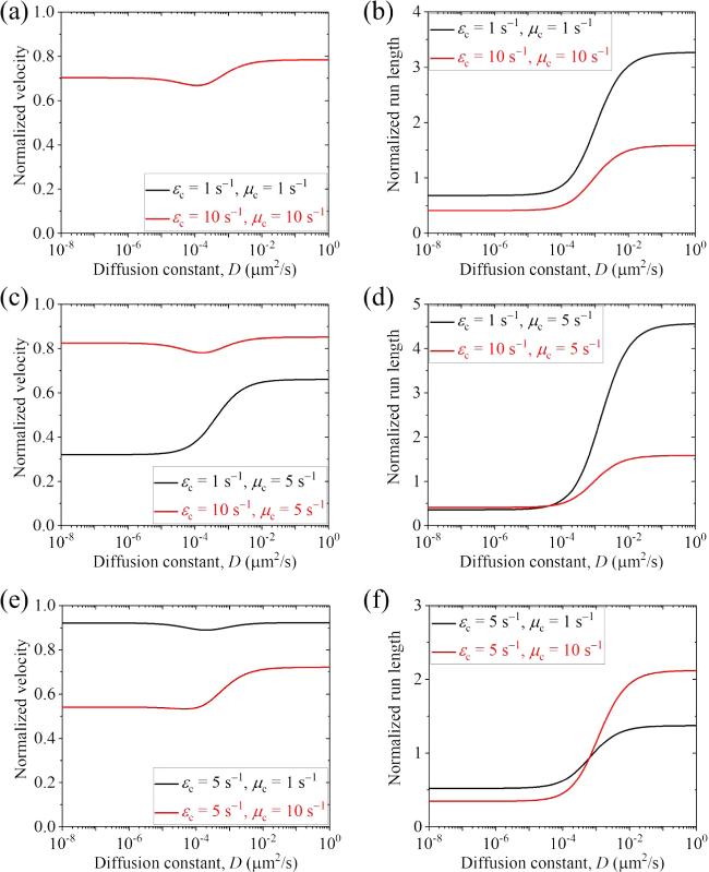
Figure 3. Normalized velocity and run length versus D for the cargo-kinesin-1 complex under different values of ${\varepsilon }_{{\rm{c}}}$ and ${\mu }_{{\rm{c}}}$, where ${\varepsilon }_{{\rm{c}}}$ is the detachment rate of the cargo when the cargo-motor complex is in the equilibrium state with no force on the cargo, ${\mu }_{{\rm{c}}}$ is the rebinding rate of the cargo when the motor is bound to the track and D is the diffusion constant of the single cargo. (a) Normalized velocity under ${\varepsilon }_{{\rm{c}}}$=1 ${{\rm{s}}}^{-1}$ and ${\mu }_{{\rm{c}}}$=1 ${{\rm{s}}}^{-1}$ (black line) and under ${\varepsilon }_{{\rm{c}}}$=10 ${{\rm{s}}}^{-1}$ and ${\mu }_{{\rm{c}}}$=10 ${{\rm{s}}}^{-1}$ (red line). Note that the two lines are identical. (b) Normalized run length under ${\varepsilon }_{{\rm{c}}}$=1 ${{\rm{s}}}^{-1}$ and ${\mu }_{{\rm{c}}}$=1 ${{\rm{s}}}^{-1}$ (black line) and under ${\varepsilon }_{{\rm{c}}}$=10 ${{\rm{s}}}^{-1}$ and ${\mu }_{{\rm{c}}}$=10 ${{\rm{s}}}^{-1}$ (red line). (c) Normalized velocity under ${\varepsilon }_{{\rm{c}}}$=1 ${{\rm{s}}}^{-1}$ and ${\mu }_{{\rm{c}}}$=5 ${{\rm{s}}}^{-1}$ (black line) and under ${\varepsilon }_{{\rm{c}}}$=10 ${{\rm{s}}}^{-1}$ and ${\mu }_{{\rm{c}}}$=5 ${{\rm{s}}}^{-1}$ (red line). (d) Normalized run length under ${\varepsilon }_{{\rm{c}}}$=1 ${{\rm{s}}}^{-1}$ and ${\mu }_{{\rm{c}}}$=5 ${{\rm{s}}}^{-1}$ (black line) and under ${\varepsilon }_{{\rm{c}}}$=10 ${{\rm{s}}}^{-1}$ and ${\mu }_{{\rm{c}}}$=5 ${{\rm{s}}}^{-1}$ (red line). (e) Normalized velocity under ${\varepsilon }_{{\rm{c}}}$=5 ${{\rm{s}}}^{-1}$ and ${\mu }_{{\rm{c}}}$=1 ${{\rm{s}}}^{-1}$ (black line) and under ${\varepsilon }_{{\rm{c}}}$=5 ${{\rm{s}}}^{-1}$ and ${\mu }_{{\rm{c}}}$=10 ${{\rm{s}}}^{-1}$ (red line). (f) Normalized run length under ${\varepsilon }_{{\rm{c}}}$=5 ${{\rm{s}}}^{-1}$ and ${\mu }_{{\rm{c}}}$=1 ${{\rm{s}}}^{-1}$ (black line) and under ${\varepsilon }_{{\rm{c}}}$=5 ${{\rm{s}}}^{-1}$ and ${\mu }_{{\rm{c}}}$=10 ${{\rm{s}}}^{-1}$ (red line). |
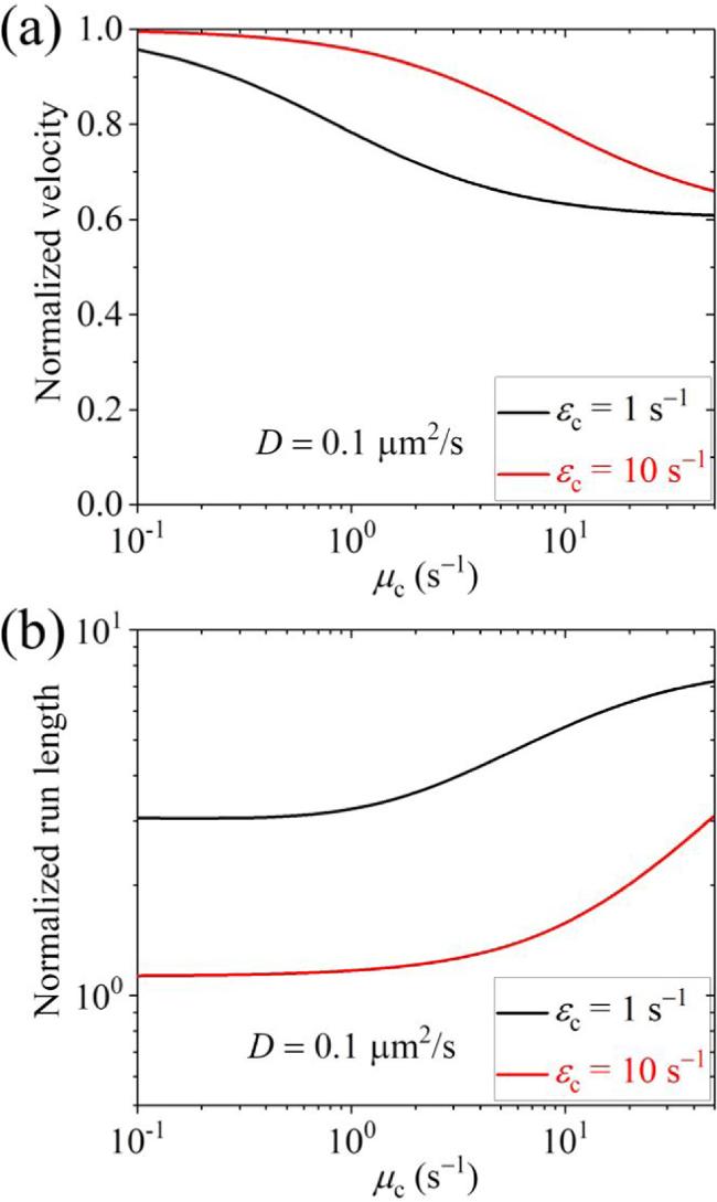
Figure 4. Normalized velocity (a) and normalized run length (b) versus ${\mu }_{{\rm{c}}}$ for the cargo-kinesin-1 complex under different values of ${\varepsilon }_{{\rm{c}}}$ and fixed D=0.1 μm2 s-1, where ${\varepsilon }_{{\rm{c}}}$ is the detachment rate of the cargo when the cargo-motor complex is in the equilibrium state with no force on the cargo, ${\mu }_{{\rm{c}}}$ is the rebinding rate of the cargo when the motor is bound to the track and D is the diffusion constant of the single cargo. |
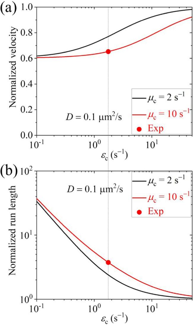
Figure 5. Normalized velocity (a) and normalized run length (b) versus ${\varepsilon }_{{\rm{c}}}$ for the cargo-kinesin-1 complex under different values of ${\mu }_{{\rm{c}}}$ and fixed D=0.1 μm2 s-1, where ${\varepsilon }_{{\rm{c}}}$ is the detachment rate of the cargo when the cargo-motor complex is in the equilibrium state with no force on the cargo, ${\mu }_{{\rm{c}}}$ is the rebinding rate of the cargo when the motor is bound to the track and D is the diffusion constant of the single cargo. Filled dots are experimental data from Henrichs et al [37], with the data in (a) being calculated from the average velocity of 918 nm s-1 for the kinesin-1 alone and the average velocity of 599 nm s-1 for the TRAK1-kinesin-1 complex (figure 2(f) in [37]) while the data in (b) being calculated from the average run length of 1.54 μm for the kinesin-1 alone and the average run length of 5.77 μm for the TRAK1-kinesin-1 complex (figure 2(d) in [37]). |
Second, we present results for the cargo-kinesin-6 complex. In figure 6 we show the normalized velocity and run length versus D for different values of ${\varepsilon }_{{\rm{c}}}$ and ${\mu }_{{\rm{c}}}$ (with some results for the occurrence probabilities of Phase I, Phase II and Phase III as well as the occurrence probabilities of Scenario I' and Scenario II' being shown in figure S5 in the Supplementary Material). It is seen, interestingly, that when D $\geqslant $ 0.1 μm2 s-1 the run length is evidently larger than that when D is small and is larger than that when the cargo has no interaction with the track, although when D $\geqslant $ 0.1 μm2 s-1 the velocity can be larger or smaller than that when D is small, which depends on the values of ${\varepsilon }_{{\rm{c}}}$ and ${\mu }_{{\rm{c}}}$. In figure 7 we show the normalized velocity and run length versus ${\mu }_{{\rm{c}}}$ for different values of ${\varepsilon }_{{\rm{c}}}$ and D=0.1 μm2 s-1. It is seen that as ${\mu }_{{\rm{c}}}$ increases, the velocity decreases and the run length changes slightly in the range of D < 50 μm2 s-1. In figure 8 we show the normalized velocity and run length versus ${\varepsilon }_{{\rm{c}}}$ for different values of ${\mu }_{{\rm{c}}}$ and D=0.1 μm2 s-1. It is seen that as ${\varepsilon }_{{\rm{c}}}$ increases, the velocity increases and the run length decreases significantly. Interestingly, it is noted that at ${\mu }_{{\rm{c}}}$=2 ${{\rm{s}}}^{-1}$ and ${\varepsilon }_{{\rm{c}}}$=4.1 ${{\rm{s}}}^{-1}$ both the normalized velocity and run length are in quantitative agreement with prior experimental data for the kinesin-6 MKLP2 motor transporting coreCPC [32], where the coreCPC is composed of full-length Survivin and Borealin with INCENP(1-100)::GFP/mCherry. At ${\mu }_{{\rm{c}}}$=2 ${{\rm{s}}}^{-1}$ and ${\varepsilon }_{{\rm{c}}}$=0.85 ${{\rm{s}}}^{-1}$ the normalized velocity is in quantitative agreement with the prior experimental data for the kinesin-6 MKLP2 motor transporting miniCPC [32], where the miniCPC is composed of full-length Survivin, Borealin and INCENP(1-100)-linker-INCENP(834-918)::GFP/mCherry that is loaded with wild-type Aurora B. In other words, with only three adjustable parameters, ${\varepsilon }_{{\rm{c}}}$=4.1 ${{\rm{s}}}^{-1}$ for the coreCPC, ${\varepsilon }_{{\rm{c}}}$=0.85 ${{\rm{s}}}^{-1}$ for the miniCPC and ${\mu }_{{\rm{c}}}$=2 ${{\rm{s}}}^{-1}$ for both the coreCPC and miniCPC, we can reproduce quantitatively the available experimental data for both the coreCPC-kinesin-6 and miniCPC-kinesin-6 complexes [32]. The results of the detachment rate of about 0.85 ${{\rm{s}}}^{-1}$ for the miniCPC being much smaller than that of about 4.1 ${{\rm{s}}}^{-1}$ for the coreCPC imply that the binding energy of miniCPC to MTs is larger than that of coreCPC, which is consistent with the experimental data showing that the miniCPC bound MTs significantly better than the coreCPC [32]. The diffusion constant being larger than 0.1 μm2 s-1 for both the coreCPC and miniCPC is also consistent with the experimental observation that both showed diffusive behaviors in vitro [32]. In addition, our results predict that the normalized run length of the miniCPC-MKLP2 complex is about 2.73 (unfilled triangle in figure 8(b)), which can be tested easily by future experiments. It is noted that since the parameter values for the kinesin-6 MKLP2 are not determined, for simplicity, in figure 8 we take the MKLP2 having the same parameter values as the Drosophila kinesin-1 except that E0 for the MKLP2 is half of that for the Drosophila kinesin-1 (see above). In fact, by taking k(+)=22.6 ${{\rm{s}}}^{-1}$ and ${\varepsilon }_{{\rm{m}}}$= 0.136 ${{\rm{s}}}^{-1}$ while other parameter values to be the same as those used to obtain the black lines in figure 8, the experimental velocity of 150 nm s-1 and run length of 1.1 μm for the MKLP2 alone can be reproduced theoretically, and the experimental velocity and run length for the MKLP2 plus coreCPC and the experimental velocity for the MKLP2 plus miniCPC can also be explained [32] (figures S6(a) and (b) in the Supplementary Material). Moreover, it is predicted that for the MKLP2 plus coreCPC Phase II with the cargo detached and the motor bound to the track is more favored while for the MKLP2 plus miniCPC Phase I with both the motor and cargo bound to the track is more favored, and for both the MKLP2 plus coreCPC and MKLP2 plus miniCPC Scenario I' with the cargo detached firstly is more favored (figures S6(c) and (d) in the Supplementary Material).
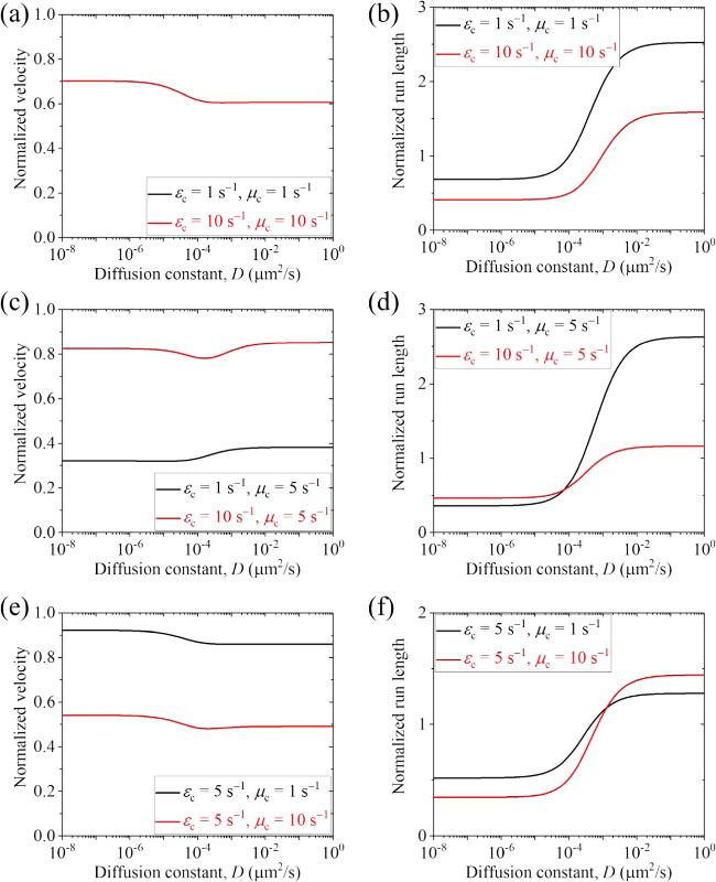
Figure 6. Normalized velocity and run length versus D for the cargo-kinesin-6 complex under different values of ${\varepsilon }_{{\rm{c}}}$ and ${\mu }_{{\rm{c}}}$, where ${\varepsilon }_{{\rm{c}}}$ is the detachment rate of the cargo when the cargo-motor complex is in the equilibrium state with no force on the cargo, ${\mu }_{{\rm{c}}}$ is the rebinding rate of the cargo when the motor is bound to the track and D is the diffusion constant of the single cargo. (a) Normalized velocity under ${\varepsilon }_{{\rm{c}}}$=1 ${{\rm{s}}}^{-1}$ and ${\mu }_{{\rm{c}}}$=1 ${{\rm{s}}}^{-1}$ (black line) and under ${\varepsilon }_{{\rm{c}}}$=10 ${{\rm{s}}}^{-1}$ and ${\mu }_{{\rm{c}}}$=10 ${{\rm{s}}}^{-1}$ (red line). Note that the two lines are identical. (b) Normalized run length under ${\varepsilon }_{{\rm{c}}}$=1 ${{\rm{s}}}^{-1}$ and ${\mu }_{{\rm{c}}}$=1 ${{\rm{s}}}^{-1}$ (black line) and under ${\varepsilon }_{{\rm{c}}}$=10 ${{\rm{s}}}^{-1}$ and ${\mu }_{{\rm{c}}}$=10 ${{\rm{s}}}^{-1}$ (red line). (c) Normalized velocity under ${\varepsilon }_{{\rm{c}}}$=1 ${{\rm{s}}}^{-1}$ and ${\mu }_{{\rm{c}}}$=5 ${{\rm{s}}}^{-1}$ (black line) and under ${\varepsilon }_{{\rm{c}}}$=10 ${{\rm{s}}}^{-1}$ and ${\mu }_{{\rm{c}}}$=5 ${{\rm{s}}}^{-1}$ (red line). (d) Normalized run length under ${\varepsilon }_{{\rm{c}}}$=1 ${{\rm{s}}}^{-1}$ and ${\mu }_{{\rm{c}}}$=5 ${{\rm{s}}}^{-1}$ (black line) and under ${\varepsilon }_{{\rm{c}}}$=10 ${{\rm{s}}}^{-1}$ and ${\mu }_{{\rm{c}}}$=5 ${{\rm{s}}}^{-1}$ (red line). (e) Normalized velocity under ${\varepsilon }_{{\rm{c}}}$=5 ${{\rm{s}}}^{-1}$ and ${\mu }_{{\rm{c}}}$=1 ${{\rm{s}}}^{-1}$ (black line) and under ${\varepsilon }_{{\rm{c}}}$=5 ${{\rm{s}}}^{-1}$ and ${\mu }_{{\rm{c}}}$=10 ${{\rm{s}}}^{-1}$ (red line). (f) Normalized run length under ${\varepsilon }_{{\rm{c}}}$=5 ${{\rm{s}}}^{-1}$ and ${\mu }_{{\rm{c}}}$=1 ${{\rm{s}}}^{-1}$ (black line) and under ${\varepsilon }_{{\rm{c}}}$=5 ${{\rm{s}}}^{-1}$ and ${\mu }_{{\rm{c}}}$=10 ${{\rm{s}}}^{-1}$ (red line). |
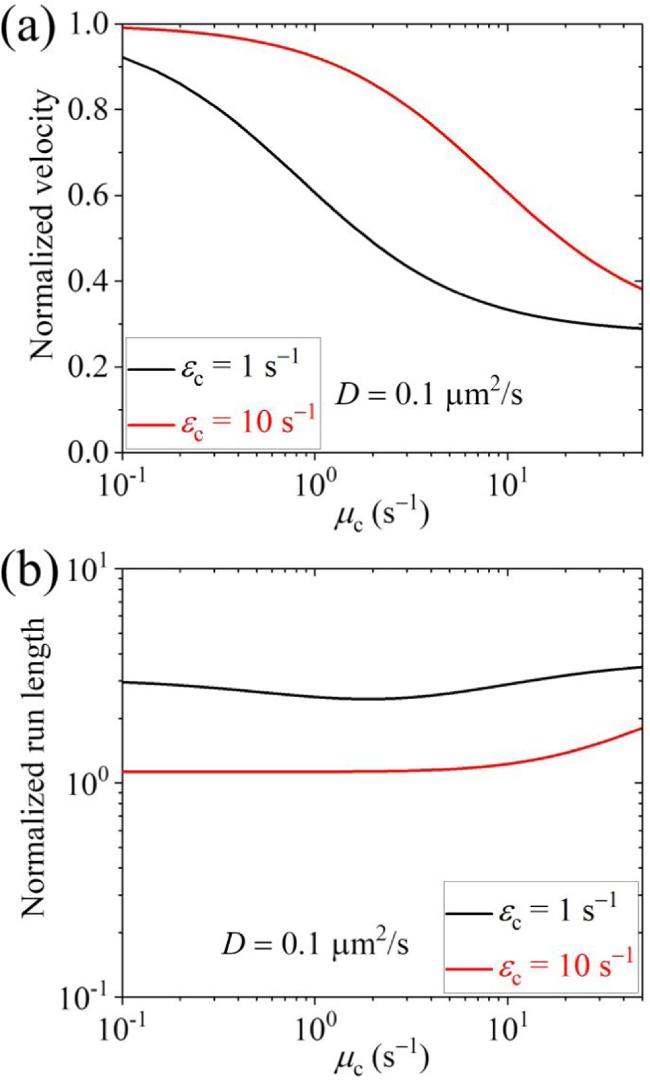
Figure 7. Normalized velocity (a) and normalized run length (b) versus ${\mu }_{{\rm{c}}}$ for the cargo-kinesin-6 complex under different values of ${\varepsilon }_{{\rm{c}}}$ and fixed D=0.1 μm2 s-1, where ${\varepsilon }_{{\rm{c}}}$ is the detachment rate of the cargo when the cargo-motor complex is in the equilibrium state with no force on the cargo, ${\mu }_{{\rm{c}}}$ is the rebinding rate of the cargo when the motor is bound to the track and D is the diffusion constant of the single cargo. |
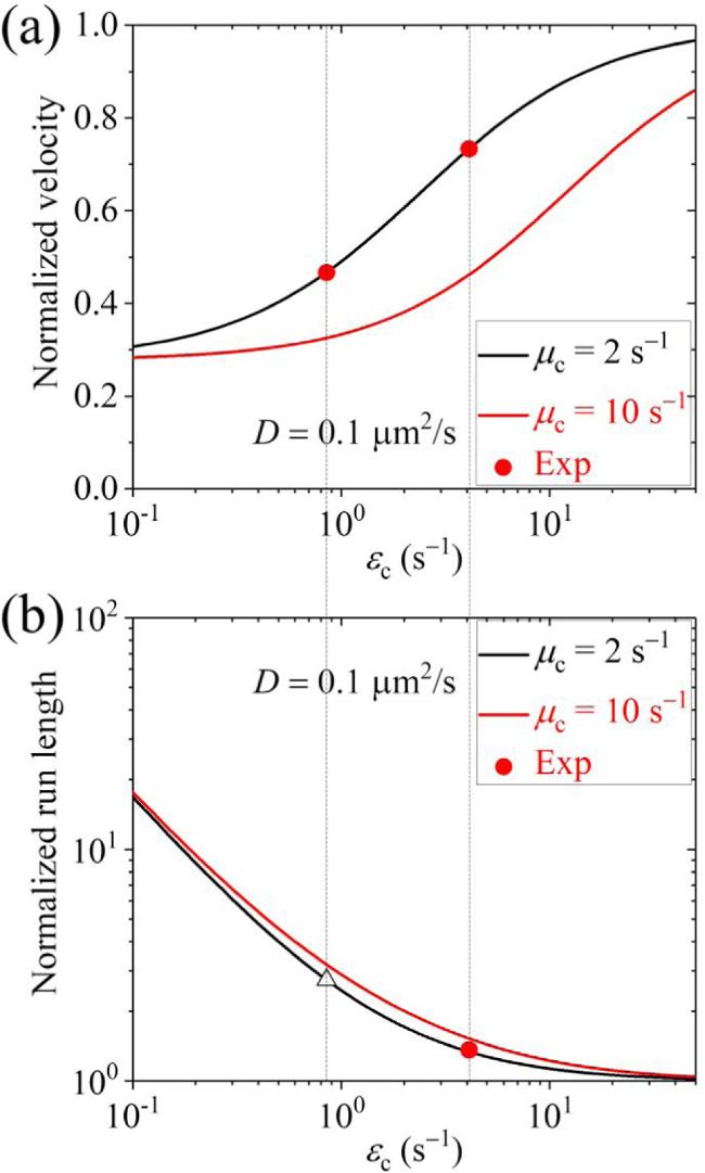
Figure 8. Normalized velocity (a) and normalized run length (b) versus ${\varepsilon }_{{\rm{c}}}$ for the cargo-kinesin-6 complex under different values of ${\mu }_{{\rm{c}}}$ and fixed D=0.1 μm2 s-1, where ${\varepsilon }_{{\rm{c}}}$ is the detachment rate of the cargo when the cargo-motor complex is in the equilibrium state with no force on the cargo, ${\mu }_{{\rm{c}}}$ is the rebinding rate of the cargo when the motor is bound to the track and D is the diffusion constant of the single cargo. Filled dots are experimental data from Adriaans et al [32], with the data in (a) being calculated from the average velocity of 0.15 μm s-1 for the kinesin-6 MKLP2 alone (figure 2(d) in [32]) and the average velocities of 0.11 μm s-1 and 0.07 μm s-1 for the MKLP2 plus coreCPC and plus miniCPC(WT), respectively (figure 2(L) in [32]) while the data (red dot) in (b) being calculated from the average run length of 1.1 μm for the MKLP2 alone and the average run length of 1.5 μm for the MKLP2 plus coreCPC (figure 2(c) in [32]). The unfilled triangle is the predicted normalized run length of the miniCPC-MKLP2 complex. |
From the results shown in figures 3 and 6, we can conclude that for the case where the cargo can diffuse on the track, with the diffusion constant D $\geqslant $ 0.1 μm2 s-1, the complex has an evidently longer run length than for the case where the cargo cannot diffuse on the track (with D=0) and has a longer run length than for the case where the cargo has no interaction with the track. Moreover, by comparing figure 3 with figure 6, it can be seen that for the kinesin-6 motor having a smaller E0 than for the kinesin-1 motor, the increase ratio of the run length for the cargo-kinesin-6 complex is smaller than that for the cargo-kinesin-1 complex. Thus, it is interesting to see if the aforementioned conclusion is still true for a kinesin motor with E0 having the value approaching zero, for example, for kinesin-7 CENP-E motor [49]. In figure 9 we show the normalized velocity and run length versus D under different values of ${\varepsilon }_{{\rm{c}}}$ and ${\mu }_{{\rm{c}}}$ for the cargo-kinesin complex with the kinesin motor having E0=0 and other parameters as those shown in table 1. From figures 3, 6 and 9 it is seen that the aforementioned conclusion is true for any cargo-kinesin complex. This gives an explanation of why the diffusion constant of a diffusive protein on MTs usually has a value close to or larger than 0.1 μm2 s-1 [50-52], for example, D=0.39 μm2 s-1 for HSET-tail [50], D=0.93 μm2 s-1 for GiKIN14a-tail [51], D=0.089 μm2 s-1 for Ndc80 [52], D=0.23 μm2 s-1 for Ska1 [52], D=0.33 μm2 s-1 for CLASP2 [52], D=1.6 μm2 s-1 for CENP-tail [52], D=0.31 μm2 s-1 for EB1 [52], etc.
Figure 9. Normalized velocity and run length versus D for the cargo-kinesin complex with the kinesin motor having E0=0 under different values of ${\varepsilon }_{{\rm{c}}}$ and ${\mu }_{{\rm{c}}}$, where ${\varepsilon }_{{\rm{c}}}$ is the detachment rate of the cargo when the cargo-motor complex is in the equilibrium state with no force on the cargo, ${\mu }_{{\rm{c}}}$ is the rebinding rate of the cargo when the motor is bound to the track and D is the diffusion constant of the single cargo. The other parameters are the same as those shown in table 1. (a) Normalized velocity under ${\varepsilon }_{{\rm{c}}}$=1 ${{\rm{s}}}^{-1}$ and ${\mu }_{{\rm{c}}}$=1 ${{\rm{s}}}^{-1}$ (black line) and under ${\varepsilon }_{{\rm{c}}}$=10 ${{\rm{s}}}^{-1}$ and ${\mu }_{{\rm{c}}}$=10 ${{\rm{s}}}^{-1}$ (red line). Note that the two lines are identical. (b) Normalized run length under ${\varepsilon }_{{\rm{c}}}$=1 ${{\rm{s}}}^{-1}$ and ${\mu }_{{\rm{c}}}$=1 ${{\rm{s}}}^{-1}$ (black line) and under ${\varepsilon }_{{\rm{c}}}$=10 ${{\rm{s}}}^{-1}$ and ${\mu }_{{\rm{c}}}$=10 ${{\rm{s}}}^{-1}$ (red line). (c) Normalized velocity under ${\varepsilon }_{{\rm{c}}}$=1 ${{\rm{s}}}^{-1}$ and ${\mu }_{{\rm{c}}}$=5 ${{\rm{s}}}^{-1}$ (black line) and under ${\varepsilon }_{{\rm{c}}}$=10 ${{\rm{s}}}^{-1}$ and ${\mu }_{{\rm{c}}}$=5 ${{\rm{s}}}^{-1}$ (red line). (d) Normalized run length under ${\varepsilon }_{{\rm{c}}}$=1 ${{\rm{s}}}^{-1}$ and ${\mu }_{{\rm{c}}}$=5 ${{\rm{s}}}^{-1}$ (black line) and under ${\varepsilon }_{{\rm{c}}}$=10 ${{\rm{s}}}^{-1}$ and ${\mu }_{{\rm{c}}}$=5 ${{\rm{s}}}^{-1}$ (red line). (e) Normalized velocity under ${\varepsilon }_{{\rm{c}}}$=5 ${{\rm{s}}}^{-1}$ and ${\mu }_{{\rm{c}}}$=1 ${{\rm{s}}}^{-1}$ (black line) and under ${\varepsilon }_{{\rm{c}}}$=5 ${{\rm{s}}}^{-1}$ and ${\mu }_{{\rm{c}}}$=10 ${{\rm{s}}}^{-1}$ (red line). (f) Normalized run length under ${\varepsilon }_{{\rm{c}}}$=5 ${{\rm{s}}}^{-1}$ and ${\mu }_{{\rm{c}}}$=1 ${{\rm{s}}}^{-1}$ (black line) and under ${\varepsilon }_{{\rm{c}}}$=5 ${{\rm{s}}}^{-1}$ and ${\mu }_{{\rm{c}}}$=10 ${{\rm{s}}}^{-1}$ (red line). |
4. Conclusion
In summary, an analytical theory is presented on the velocity and run length of the molecular motor transporting track-interacted cargo. The theory is then applied to the TRAK1-kinesin-1 and CPC-kinesin-6 complexes. The theoretical results explain quantitatively the prior experimental data on the velocity and run length of the TRAK1-kinesin-1 and CPC-kinesin-6 complexes. Interestingly, it is found that for the case where the cargo can diffuse on the track, with the diffusion constant D $\geqslant $ 0.1 μm2 s-1, the complex not only has a longer run length than for the case where the cargo has no interaction with the track but also has an evidently longer run length than for the case where the cargo cannot diffuse on the track.
Acknowledgments
This work was supported by the Youth Project of Science and Technology Research Program of Chongqing Education Commission of China (No. KJQN202404522).