


1. Overview/motivation
Two major revolutions occurred during the development of superstring theory. In the so-called first superstring revolution (1984-1985), five perturbatively consistent quantum superstring theories were established, namely, type IIA, type IIB, type I, heterotic SO(32) and heterotic E8 × E8. Each of these theories Requires 10 spacetime dimensions (nine spatial and one temporal) and spacetime supersymmetry (SUSY). In the so-called second string revolution, many non-perturbative states were discovered, now known as p-branes or Neveu-Schwarz (NS) NS p-branes and Dirichlet p (Dp) branes. These played an important role in this revolution, giving rise to various dualities and revealing the existence of a unique though not-yet completely established unified theory called M-theory (See [1] for example).
M-theory has a maximal 11-dimensional spacetime and unifies not only the five known 10-dimensional perturbative string theories but also the previously isolated 11-dimensional supergravity. These latter six theories appear as six different limits of the former at six different limits, as shown in figure 1.
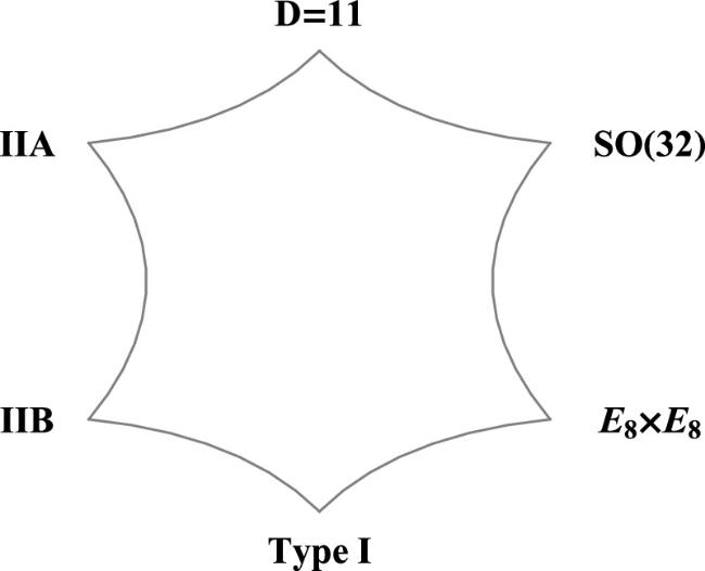
Figure 1. M-theory. |
It also answers many of the puzzles that remained after the first string revolution, such as the so-called ‘embarrassment of riches' problem (too many string theories and one real world) problem and the status of 11-dimensional supergravity. In particular, Dp-branes have a dual description either in terms of closed or open strings, which provides the basis for the anti-de Sitter (AdS)/conformal field theory (CFT) as well as the matrix theory proposal for M-theory.
1.1. The first superstring revolution
In the early days of superstrings and supermembranes, two views were taken in the world of quantum gravity and grand unified theory.
People in the string community (mainly in the US) at that time were strongly opposed to the study of supermembranes, i.e., extended objects with spatial dimensionality higher than one, for the simple reason that only strings, as (1 + 1)-dimensional CFTs, could potentially be first quantized due to the presence of sufficient underlying local symmetries. In particular, Weyl symmetry along with the two worldsheet diffeomorphisms can be used to make the worldsheet flat in a given coordinate patch, implying that there is no worldsheet physical propagating gravity or that the worldsheet propagating gravity is decoupled.
This was reflected, for example, in the first well-known ‘Superstring Theory' textbook by Green, Schwarz and Witten with the quotation [2] ‘Weyl invariance, or at least the ability to locally gauge away the hαβ dependence, is central in the physics of strings. This is one of the things that singles out strings as opposed to, say, membranes. Membranes and objects of still higher dimensionality have another glaring problem, as follows. Equation (1 ) (i.e., the p-brane Polyakov-type action) defines an (p + 1)-dimensional quantum field theory, which is by power counting renormalizable for p=1 and non-renormalizable for p > 1. Making sense of (1 ) as a quantum theory for p > 1 is as difficult a problem as making sense of general relativity as a quantum theory. Thus, membranes or higher dimensional objects would be hardly be a promising start toward quantum gravity'.
$\begin{eqnarray}\begin{array}{rcl}{S}_{p} & =& -\frac{{T}_{p}}{2}\displaystyle \int {{\rm{d}}}^{p+1}\sigma \sqrt{-h}\\ & & \times \,\left({h}^{\alpha \beta }{\partial }_{\alpha }{X}^{\mu }{\partial }_{\beta }{X}^{\nu }{g}_{\mu \nu }(X)-(p-1)\right).\end{array}\end{eqnarray}$
Meanwhile, those in Europe, mostly in England, took a different view by asking if people are interested in strings, why not higher-dimensional extended objects for quantum gravity? There are several rationales behind this view.
When Green and Schwarz (GS) used the so-called fermionic local κ-symmetry, discovered by Warren Siegel from the supersymmetric particle action [3], to derive type I and type II superstring theories with manifest spacetime supersymmetries without the need of Gliozzi-Scherk-Olive (GSO) projection, called the Green-Schwarz formalism of superstring theories, a certain γ-matrix identity must hold that can be true in spacetime dimension D=10, 6, 4 and 3, corresponding to those dimensions for which the super Yang-Mills theories exist. This led to the belief that this κ-symmetry would be difficult to achieve for the worldvolume actions of objects with spatial dimensionality higher than one, while still possessing their respective manifest spacetime supersymmetries.
It was the late Polchinski and his collaborators who overcame this challenge by showing explicitly that this local fermionic symmetry can be used to construct the supermembrane (actually a super 3-brane) action in six spacetime dimensions [4].
Shortly after this and following the same procedure, Bergshoeff, Sezgin and Townsend [5] found corresponding actions for other values of d and D, called super p-branes where p=d-1 is the number of spatial dimensions of the worldvolume (here D stands for the spacetime dimensions). For example, for the 11-dimensional supermembrane action, they showed that the κ-symmetry itself requires that 11-dimensional supergravity must be on-shell, i.e., the equations of motion (EOMs) of 11-dimensional supergravity hold, when the supermembrane couples with the supergravity.
This, to some extent, hints that the 11-dimensional supergravity multiplet may give rise to the massless modes of the supermembrane if the latter can be quantized.
Soon after this, the Polyakov-type actions for a large class of super p-branes in diverse dimensions were classified [6]. Each of their actions needs κ-symmetry and this symmetry can hold only if the corresponding supergravity fields satisfy certain constraints consistent with their EOMs when the p-brane is coupled with the supergravity background.
Moreover, Duff, Howe, Inami and Stelle [7] showed how the action for a (p-1)-brane in (D-1)-dimensions could be derived from that for a p-brane in D-dimensions via the so-called double-dimensional reduction. In particular, the type IIA superstring action in 10 dimensions can be obtained from the supermembrane action in 11 dimensions.
Precisely because of these developments, there was a surge of interest in super p-branes, particularly the 11-dimensional supermembrane, even though these higher-dimensional objects do not appear to be quantizable.
Each of these super p-branes considers only its worldvolume scalar supermultiplet, i.e., consisting of only the worldvolume scalars and spinors in the multiplet. As mentioned above, they were classified in diverse dimensions in [6]. According to this classification, type II p-branes, i.e., those with N=2 spacetime SUSY, do not exist for p > 1, which can be summarized in the so-called old brane scan [8], as shown in figure 2.
Figure 2. The old brane scan. |
Following the above, two puzzles remain. If 10-dimensional superstrings are the whole story, how can we explain and understand 11-dimensional supergravity, noting that the dimensional reduction of 11-dimensional supergravity gives rise to type IIA supergravity. In addition, as mentioned above, Duff, Howe, Inami and Stelle [7] demonstrated that the type IIA superstring action can be obtained from the 11-dimensional supermembrane action via the so-called double-dimensional reduction.
In other words, the 11-dimensional supermembrane appears to be more fundamental than the superstring. If the type IIA superstring can be quantized, plus its connection to the 11-dimensional supermembrane, it hints that there should be a quantum theory for the 11-dimensional supermembrane. This sparked interest in seeking how to quantize the supermembrane.
Among these efforts, the matrix regularization procedure stands out. Its basic ideas are: Using the three diffeomorphisms of the M2 brane worldvolume, one can set its worldvolume metric ${h}_{0a}=0,\,{h}_{00}\propto -\det {h}_{ab}$ with a, b=1, 2. In addition, the light-cone gauge of X+ ∝ τ is taken.
With the above gauge choices, the residual symmetries of the M2 worldvoume are the diffeomorphisms preserving the area of the M2. As such, any function defined on the M2 worldvolume can be represented by a U(N) matrix with N →∞, and the dynamics of M2 can then be described by the following Hamiltonian
$\begin{eqnarray}\begin{array}{rcl}H & =& \frac{1}{2\pi {l}_{11}^{3}}{\rm{Tr}}\left(\frac{1}{2}{\dot{X}}^{i}{\dot{X}}^{i}-\frac{1}{4}\left[{X}^{i},{X}^{j}\right]\left[{X}^{i},{X}^{j}\right]\right.\\ & & \left.+\,\frac{1}{2}{\theta }^{T}{\gamma }^{i}\left[{X}^{i},\theta \right]\right),\end{array}\end{eqnarray}$
where l11 is the 11-dimensional Planck length, Xi (i=1, 2, ⋯ 9) and the nine-dimensional Majorana spinor θ are all N × N matrices.
By this, we convert the (1 + 2)-dimensional M2 brane dynamics to (1 + 0)-dimensional infinite Matrix quantum mechanics, which appears to be quantizable [9], therefore providing hope for quantizing the supermembrane.
However, not long after this, de Wit, Luscher and Nicolai [10] showed that the energy spectrum of this system is continuous, suggesting the instability of this system, therefore ending people's further interest in studying the 11-dimensional supermembrane.
One had to wait about 10 years, when the non-perturbative effects of superstrings were considered and became important, to realize the physical significance of this continuous spectrum.
The would-be first-quantized matrix theory turns out to be a second-quantized one, containing multi-particle and multi-brane states. Therefore the continuous spectrum problem is solved and the resulting matrix theory provides a concrete proposal for M-theory [11] (see also the insightful review article by Taylor [12]).
In addition to the above, by the end of the first superstring revolution, other problems were encountered, such as the so-called 'embarrassment of riches' (too many theories but one real world) experimental testing problem1. All of the five superstring theories are only perturbatively well-defined. In other words, they are only asymptotically well-defined. A well-defined unified theory cannot be an asymptotic one, as its coupling, vacuum structures and other characteristics, except for some fundamental inputs such as its tensions, constants and some initial or boundary conditions, should all be determined dynamically.
Addressing any of these issues needs to go to the non-perturbative region of superstrings, i.e., ${g}_{s}\sim { \mathcal O }(1)$.
The worldsheet action of a superstring can be used to study its perturbative behaviors. However, studying its non-perturbative effects remained a challenging problem. We did not have a non-perturbative formulation of a given superstring theory; the only thing available at that time was the corresponding 10-dimensional supergravity, which was believed to be the low-energy effective theory of the perturbative superstring2 .
This is because, for each of the five perturbative superstring theories, the massless spectrum corresponds to the corresponding supergravity supermultiplet, plus a possible super Yang-Mills multiplet (such as in the type I and the two heterotic string theories).
For example, in the type IIA theory, the massless spectrum can be given as the tensor product of left and right movers with their eight-spinors having opposite chirality as
$\begin{eqnarray}\begin{array}{l}({8}_{v}\displaystyle \oplus {8}_{s})\displaystyle \otimes ({8}_{v}\displaystyle \oplus {8}_{c})\\ \quad ={8}_{v}\displaystyle \otimes {8}_{v}\displaystyle \oplus {8}_{v}\displaystyle \otimes {8}_{c}\displaystyle \oplus {8}_{s}\displaystyle \otimes {8}_{v}\displaystyle \oplus {8}_{s}\displaystyle \otimes {8}_{c}.\end{array}\end{eqnarray}$
Here, the bosonic NSNS sector gives the gravity multiplet and decomposes according to the little group SO(8) as
$\begin{eqnarray}{8}_{v}\otimes {8}_{v}=1\oplus 28\oplus 35=\phi \oplus {B}_{ij}\oplus {g}_{ij},\end{eqnarray}$
where Φ is a singlet (the dilaton), Bij is a 2-form antisymmetric tensor (the Kalb-Ramond field) and gij is the traceless symmetric tensor (the graviton) all under SO(8). While the so-called Ramond-Ramond (RR) sector gives the additional bosonic form potentials from the bi-linear fermionic fields with opposite chirality as $\begin{eqnarray}{8}_{s}\otimes {8}_{c}=8\oplus 56={A}_{i}\oplus {A}_{ijk},\end{eqnarray}$
where Ai is a 1-form vector while Aijk is a 3-form tensor. Concretely, we have $\begin{eqnarray}{\psi }_{a}{\tilde{\psi }}_{\dot{a}}={\gamma }_{a\dot{a}}^{i}{A}_{i}+\frac{1}{3!}{\gamma }_{a\dot{a}}^{ijk}{A}_{ijk}.\end{eqnarray}$
For a type IIB superstring, its massless spectrum comes from the tensor product of left and right movers with the fermions having the same chirality as $\begin{eqnarray}\begin{array}{l}({8}_{v}\displaystyle \oplus {8}_{s})\displaystyle \otimes ({8}_{v}\displaystyle \oplus {8}_{s})\\ \,=\,{8}_{v}\displaystyle \otimes {8}_{v}\displaystyle \oplus {8}_{v}\displaystyle \otimes {8}_{s}\displaystyle \oplus {8}_{s}\displaystyle \otimes {8}_{v}\displaystyle \oplus {8}_{s}\displaystyle \otimes {8}_{s}.\end{array}\end{eqnarray}$
The bosonic NSNS sector remains the same as in type IIA case, while the bosonic RR sector also gives additional bosonic form potentials as $\begin{eqnarray}{8}_{s}\otimes {8}_{s}=1\oplus 28\oplus 3{5}_{+}=\chi \oplus {A}_{ij}\oplus {A}_{ijkl}^{+},\end{eqnarray}$
where χ a zero-form scalar, an axion-like field, Aij is a 2-form tensor and ${A}_{ijkl}^{+}$ is a 4-form tensor, satisfying the following self-duality $\begin{eqnarray}{A}_{{i}_{1}{i}_{2}{i}_{3}{i}_{4}}^{+}=\frac{1}{4!}{\epsilon }_{{i}_{1}{i}_{2}{i}_{3}{i}_{4}}{\,}^{{i}_{5}{i}_{6}{i}_{7}{i}_{8}}{A}_{{i}_{5}{i}_{6}{i}_{7}{i}_{8}}^{+},\end{eqnarray}$
which reduces its degrees of freedom (DOF) by half. Concretely, we have $\begin{eqnarray}{\psi }_{a}{\tilde{\psi }}_{b}={({\gamma }^{9})}_{ab}\chi +\frac{1}{2!}{({\gamma }^{ij})}_{ab}{A}_{ij}+\frac{1}{4!}{({\gamma }^{ijkl})}_{ab}{A}_{ijkl}^{(+)}.\end{eqnarray}$
In the above, γi with i=1, 2, ⋯ 8 are the SO(8) Dirac matrices and γ9 ≡ γ1γ2 ⋯ γ8 the eight-dimensional chiral operator.The NSNS 2-form potential B2 appears in any consistent superstring theory (except for type I) and is always with the gravity multiplet, i.e., the NSNS sector. Its appearance is completely expected since the string carries the so-called NSNS charge and, as a one-dimensional extended object, it must couple with a 2-form potential just like a point-charge must couple with a U(1) 1-form potential, given what we have discussed previously.
The RR form potentials in either IIA or IIB come from the bi-linear spinors and it is difficult to understand their origins from a perturbative string perspective, although it is clear that the NSNS 2-form potential B2 couples to the underlying fundamental string. Even so, the natural question of what the magnetic dual of a string in 10 dimensions is, supposedly an NSNS five-brane, had never been asked until the very end of the 1980s, when a very few researchers, including myself, began seriously addressing the non-perturbative issues concerning how strings are related to other higher-dimensional objects.
Michael Duff [14] was the first to notice that there may be a duality between a heterotic string with either SO(32) or E8 × E8 and the corresponding so-called heterotic five-brane, thereby conjecturing the existence of the heterotic five-brane. This was based, among other things, on the observation that there are two equivalent dual formulations of N=1 supergravity plus the respective super Yang-Mills in 10 dimensions: one with the NSNS 3-form field strength or 2-form NSNS potential [15], associated with the heterotic string, and the other with the NSNS 7-form field strength or 6-form potential [16] associated with the so-called heterotic five-brane. The first non-trivial evidence in support of this was made by Strominger [17] in finding the heterotic five-brane, with its core as an instanton, from the low-energy theory of heterotic strings, as a solution preserving one half of the spacetime SUSY3 . Subsequently, Duff and I [18] found the so-called elementary five-brane solution from the 10-dimensional N=1 supergravity, which also preserves 1/2 spacetime SUSY and was shown to correspond to the zero-size instanton limit of Strominger's solution. Moreover, this five-brane solution solves the respective EOMs of all of the 10-dimensional supergravities and preserves the respective 1/2 spacetime supersymmetries; therefore serving as a 1/2 Bogomol'nyi-Prasad-Sommerfield (BPS) five-brane solution of the respective supergravities. All these studies provide further evidence in support of the existence of NSNS five-branes.
The discovery of various supergravities actually predates the corresponding perturbative superstrings by a few years. They are based on the representations of the underlying SUSY algebra and the spacetime localization of the corresponding SUSY transformations. Since the algebra itself has nothing to do with the string coupling, each supergravity theory, whose concrete form is tied to the relevant low-energy scale (the corresponding Planck scale), as in every effective theory description4 , should be viewed as the low-energy effective theory of the underlying non-perturbative string/M-theory, rather than, as previously thought, that of the perturbative one, see a discussion of this in [20].
1.2. The second superstring revolution
In other words, if supergravities are the respective low-energy effective theories of the underlying non-perturbative superstrings (independent of the underlying string coupling or in other words, valid for any string coupling), we can simply ignore the perturbative picture regarding the RR potentials (named in the perturbative sense) discussed earlier and naturally associate each of them with the corresponding branes. This is just like a point charge coupled with a 1-form potential, a one-dimensional charged string coupled with a 2-form potential and, in general, a p-dimensional charged brane coupled with a (1 + p)-form potential5 . In other words, in general, we have the following:
$\begin{eqnarray}\begin{array}{rcl}{A}_{1} & =& {A}_{\mu }{\rm{d}}{x}^{\mu }\\ & & \,\to \qquad \qquad \qquad \quad \,\rm{coupled\,with\,a\,charged\,point\,particle}\,,\\ {A}_{2} & =& \displaystyle \frac{1}{2!}{A}_{\mu \nu }{\rm{d}}{x}^{\mu }\wedge {\rm{d}}{x}^{\nu }\\ & & \,\to \qquad \qquad \quad \,\rm{coupled\,with\,a\,charged\unicode{x000A0}1-brane}\,,\\ {A}_{3} & =& \displaystyle \frac{1}{3!}{A}_{\mu \nu \rho }{\rm{d}}{x}^{\mu }\wedge {\rm{d}}{x}^{\nu }\wedge {\rm{d}}{x}^{\rho }\\ & & \,\to \quad \quad \,\rm{coupled\,with\,a\,charged\unicode{x000A0}2-brane}\,,\\ & & \quad \vdots \\ {A}_{1+p} & =& \displaystyle \frac{1}{(1+p)!}{A}_{\mu \cdots \sigma }{\rm{d}}{x}^{\mu }\wedge \cdots \wedge {\rm{d}}{x}^{\sigma }\\ & & \,\to \quad \rm{coupled\,with\,a\,charged\unicode{x000A0}p-brane,}\,\end{array}\end{eqnarray}$
To demonstrate the correctness of the above, we need to show the existence of these branes associated with the form potentials in various supergravities along with the fundamental string which is associated with the NSNS 2-form B2 by finding their solutions from these supergravities and at the same time to show that their existence is independent of the string coupling.
Duff and I were among the first to start such a journey to find the brane solutions or string solitons preserving one half of spacetime SUSY, called 1/2 BPS branes. For example, Duff and I found the so-called elementary five-brane (i.e., the NSNS 5-brane) [18] mentioned earlier, the self-dual superthreebrane (the D3 brane) [21] and the general 1/2 BPS p-branes in diverse dimensions [22]. Note that the fundamental string, or F-string, is also a 1/2 BPS state, as identified earlier [23]. See also the discussions in [24] for 1/2 BPS NSNS 5-brane solitons and in particular their zero modes in type II superstrings. The black p-brane solutions in 10 dimensions were also found in [25].
Although these 1/2 BPS p-branes are found as solutions of various supergravities, their existence is independent of the underlying string coupling and they are fundamental dynamical objects of non-perturbative string/M-theory. This is because their respective Arnowitt-Deser-Misner (ADM) mass per unit brane volume or their tension [26] equaling their corresponding charge, i.e., Mp=Qp in certain units (the BPS property), is protected by the underlying unbroken SUSY and the quantized charge. In other words, this relation is exact and independent of the underlying string coupling, or in other words is suitable for any string coupling6 . For example, the existence of these 1/2 BPS objects can also be deduced purely from their respective SUSY algebra with the proper central extension [27-29] and this also shows that these objects are the fundamental objects in the underlying non-perturbative theory following [30].

Figure 3. The new brane scan. All possible d ≥ 2 scalar supermultiplets, denoted by circles, and vector supermultiplets, denoted by crosses, according to D=d+ the number of scalars. |
All these 1/2 BPS p-branes are the string solitons of the non-perturbative superstring theory and they are the corresponding non-perturbative superstring states. Just like the fundamental string or F-string, they are the basic dynamical objects of the complete non-perturbative string theory. These objects, including the strings, are all intrinsically connected to each other. This discovery puts an end to the early assertion that strings have nothing to do with other branes. In other words, if one wants to study strings, the dynamics of other branes cannot be ignored in general and vice versa.
For type II in D=10, the newly discovered p-branes, except for the type IIA NSNS 5-branes (also the D=11 M5 brane) whose worldvolume modes give a tensor supermultiplet, are all vector supermultiplets, i.e., the supersymmetric Yang-Mills theory. These are nowadays called D-branes.
Almost at the same time, Polchinski et al [32] discovered these branes, but via a completely different approach that was not widely accepted at the time. The branes found by the two different approaches were not recognized as the same until the surge of the so-called second string revolution around 1995. This was still due to the late Polchinski [33,34].
Polchinski et al [32] applied T-duality, derived from closed string theory, to directly open strings. This application requires the existence of D-branes. Initially, this was met with skepticism, as open strings are unable to wind around compact directions with the respective conserved winding numbers and, further, the required hyperplanes identified as D-branes for consistency have no place in perturbative string theory. This led to a prejudice within the string community against the existence of higher-dimensional branes. As such, the validity of this direct application of T-duality to open strings was questioned at that time.
T-duality for closed strings in the simplest case can be understood as follows. Consider a closed string moving along a compactified circle with radius R and the other one along a compactified circle with radius $\tilde{R}$, and the respective string winding number around the circles as $w,\tilde{w}$. If $R\tilde{R}={\alpha }^{{}^{{\prime} }}$ with the string slope parameter ${\alpha }^{{}^{{\prime} }}$ and we make the exchanges of $n\leftrightarrow \tilde{w}$ and $w\leftrightarrow \tilde{n}$, then these two string theories are either equivalent (as in the case of bosonic string theory) or one string theory is mapped to the other one (as in IIA and IIB).
From the perspective of the string worldsheet, T-duality is nothing but the worldsheet electromagnetic or Hodge duality. If we apply this to an open string, it has the following consequences for its boundary conditions
$\begin{eqnarray}\rm{Neumann\,BC}\,\,\iff \,\,\rm{Dirichlet\,BC}\,.\end{eqnarray}$
In other words, if we perform T-duality along a direction for which the open string initially obeys the Neumann boundary condition, it will obey the Dirichlet one after this duality and vice versa. In other words, the two ends of an open string after certain number of such T-dualities will obey the Dirichlet boundary condition along these T-duality directions and the Neumann boundary condition along the rest directions. Therefore, the Dirichlet boundary conditions obeyed by the ends of the open string define the location of a hyperplane, on which the ends of the open string can move freely, along these Dirichlet directions.The discovery of the string solitons associated with RR potentials not only validates Polchinski et al's application of the T-duality found from closed strings to open strings, but also reveals the existence of D-branes in string theories.
The discovery of D-branes by Polchinski et al [32,33] via the open string T-duality, with respect to string solitons, has an advantage and usefulness in that in weak string coupling, the open string so defined provides a perturbative description for the non-perturbative D-branes and this appears to be the first case in the history of physics where a perturbative description of the underlying non-perturbative objects can be provided in the region of small coupling. We know that the massless modes of the open string correspond to supersymmetric Yang-Mills theory, which is also consistent with what has been found as the zero modes of the solitonic D-branes that form the corresponding vector supermultilets.
In summary, finding the stringy extended solitons, i.e. the 1/2 BPS p-branes, from various supergravities, has the following significances: 1) establishing the intrinsic connection among these branes, including the fundamental strings; 2) validating the use of the open string T-duality and as such leading to a useful description of the D-brane solitons in terms of perturbative open strings when the string coupling is weak; 3) providing the basis for the AdS/CFT correspondence.
Moreover, this finding provides a basis for various string dualities, which always exchange the fundamental string with its solitons, and plays an important role in the existence of a unified theory called M-theory [1].
By now, we hope that we have provided enough physical motivation to convince the reader that finding the so-called 1/2 BPS basic extended objects associated with the various form potentials in various supergravities is extremely important for understanding the non-perturbative properties of the underlying unified theory, since these objects can be used to explore this unknown theory.
Without further ado, we will focus on finding these 1/2 BPS extended objects from various supergravities with maximal number of SUSY in diverse dimensions. For those BPS extended solutions from supergravities with fewer SUSYs and other aspects of these solutions in diverse dimensions, we refer to the reader to, for example, [36-38]. For black brane solutions and non-BPS solutions7 , refer to [25] for black brane solutions in 10 dimensions, [22,31,36-38] for black p-brane solutions in diverse dimensions and [39] for non-supersymmetric p-brane solutions including non-BPS ones in diverse dimensions.
2. The brane sigma-model action
Before moving on to find the 1/2 BPS p-branes, we briefly introduce the bosonic part of the supersymmetric p-brane sigma-model action for those branes in the old brane scan. This bosonic part is also useful for finding brane solutions from supergravities for the branes in the new brane scan, because as far as the static SUSY-preserving 1/2 BPS p-brane is concerned, the other worldvolume fields, such as the possible vector or tensor along with the fermionic ones, are not excited and can therefore be set to vanish.
Just as a point particle moving in spacetime gives a worldline, a string moving in spacetime gives a (1 + 1)-dimensional worldsheet and a general p-brane moving in spacetime gives a (1 + p)-dimensional worldvolume, see figure 4 for an illustration.
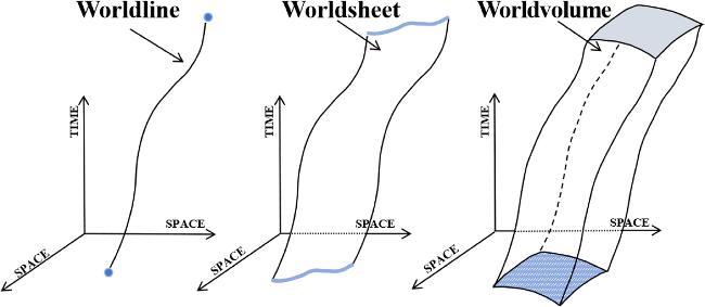
Figure 4. Particles, strings and branes. |
For those super p-branes in the old brane scan, the worldvolume action of a super p-brane moving in a curved superspace with a superspace coordinate ZM=(xμ, θα) is [5,6]
$\begin{eqnarray}\begin{array}{rcl}{S}_{d} & =& {T}_{d}\displaystyle \int {{\rm{d}}}^{d}\sigma \left(-\frac{1}{2}\sqrt{-\gamma }{\gamma }^{ij}{E}_{i}{\,}^{a}{E}_{j}{\,}^{b}{\eta }_{ab}+\frac{d-2}{2}\sqrt{-\gamma }\right.\\ & & \left.+\,\frac{1}{d!}{\epsilon }^{{i}_{1}\cdots {i}_{d}}{E}_{{i}_{1}}{\,}^{{A}_{1}}\cdots {E}_{{i}_{d}}{\,}^{{A}_{d}}{C}_{{A}_{1}\cdots {A}_{d}}\right),\end{array}\end{eqnarray}$
where the first term is the usual kinetic or the volume term determined by the metric, the second the cosmology one and the third the Wess-Zumino or volume one determined by the total antisymmetric density ${\epsilon }^{{i}_{1}\cdots {i}_{d}}$.In the above, EM A is the supervielbein with the superspace world indices M=μ, α and the tangent space indices A=a, α. We also define the worldvolume pull-back as Ei A=∂iZMEM A with i, j=0, 1, ⋯ p the worldvolume indices. Note here d=1+p, μ=0, 1 ⋯ D-1 with D the spacetime dimension and α the spinor indices of the spacetime spinor coordinate θ. ${C}_{{A}_{1}\cdots {A}_{d}}(Z)$ is the super d-form potential.
The target-space symmetries of this action are super diffeomorphisms, Lorentz invariance and d-form gauge invariance. The worldvolume symmetries are ordinary diffeomorphisms and the κ-symmetry, which is defined as
$\begin{eqnarray}\delta {Z}^{M}{E}_{M}{\,}^{a}=0,\quad \delta {Z}^{M}{E}_{M}{\,}^{\alpha }={(1+{\rm{\Gamma }})}^{\alpha }{\,}_{\beta }{\kappa }^{\beta },\end{eqnarray}$
with $\begin{eqnarray}{{\rm{\Gamma }}}^{\alpha }{\,}_{\beta }=\frac{{(-)}^{d(d-3)/4}}{d!\sqrt{-\gamma }}{\epsilon }^{{i}_{1}\cdots {i}_{d}}{E}_{{i}_{1}}{\,}^{{a}_{1}}\cdots {E}_{{i}_{d}}{\,}^{{a}_{d}}{\left({{\rm{\Gamma }}}_{{a}_{1}\cdots {a}_{d}}\right)}^{\alpha }{\,}_{\beta }.\end{eqnarray}$
If we focus on the bosonic part of the above action (13 ), it gives
$\begin{eqnarray}\begin{array}{rcl}{S}_{d} & =& {T}_{d}\displaystyle \int {{\rm{d}}}^{d}\sigma \left(-\frac{1}{2}\sqrt{-\gamma }{\gamma }^{ij}{\partial }_{i}{X}^{\mu }{\partial }_{j}{X}^{\nu }{G}_{\mu \nu }(X)+\frac{d-2}{2}\sqrt{-\gamma }\right.\\ & & \left.+\,\frac{1}{d!}{\epsilon }^{{i}_{1}\cdots {i}_{d}}{\partial }_{{i}_{1}}{X}^{{\mu }_{1}}\cdots {\partial }_{{i}_{d}}{X}^{{\mu }_{d}}{C}_{{\mu }_{1}\cdots {\mu }_{d}}\right),\end{array}\end{eqnarray}$
where Gμν is the background metric in the so-called p-brane frame (its relation with the Einstein frame metric will be given later) and ${C}_{{\mu }_{1}\cdot {\mu }_{d}}$ is the d-form potential.The above action reminds that a p-dimensional object, when it carries a U(1) charge, must couple with a (1 + p)-form potential when the U(1) local symmetry is insisted. It is clear that action (16 ) is invariant up to a surface term (the EOM is invariant) under the gauge transformation
$\begin{eqnarray}{C}_{d}\to {C}_{d}^{{\prime} }={C}_{d}+{\rm{d}}{{\rm{\Lambda }}}_{d-1},\end{eqnarray}$
where the (d-1)-form λd-1 is the gauge transformation parameter.This is just like in quantum electrodynamics. A local U(1) symmetry must imply that a U(1) charged particle (or object) couples with the U(1) gauge potential (or higher-form gauge potential) for consistency.
Noether's theorem says that a global U(1) symmetry gives a conserved charge. If this symmetry can be promoted to a local one, i.e., a U(1) gauge symmetry, there must exist a U(1) form gauge potential associated with the corresponding conserved current for consistency and their interaction can also be easily determined via the standard current and gauge potential coupling or the minimal coupling.
Let us see how the Wess-Zumino action is obtained from this coupling. For a point charge q moving in bulk spacetime along its worldline Xμ(τ), the current produced by this charge at a spacetime point x is
$\begin{eqnarray}\begin{array}{rcl}{j}^{\mu }(x) & =& q\displaystyle \int {\rm{d}}\tau \,{\partial }_{\tau }{X}^{\mu }(\tau )\,{\delta }^{(D)}\left(x-X(\tau )\right),\end{array}\end{eqnarray}$
then the coupling is given by jμ(x)Aμ(x) and the Wess-Zumino action is given as $\begin{eqnarray}\begin{array}{rcl}{S}_{\mathrm{WZ}} & =& \int {{\rm{d}}}^{D}x\,{j}^{\mu }(x){A}_{\mu }(x)\\ & =& q\int {\rm{d}}\tau \,{\partial }_{\tau }{X}^{\mu }(\tau ){A}_{\mu }(X).\end{array}\end{eqnarray}$
For a string with its line charge density μ1 moving in bulk spacetime with its worldsheet Xμ(τ, σ), the current produced at a given spacetime point x is
$\begin{eqnarray}{j}^{\mu \nu }(x)={\mu }_{1}\int {{\rm{d}}}^{2}\sigma \,{\epsilon }^{{ij}}{{\rm{\partial }}}_{i}{X}^{\mu }{{\rm{\partial }}}_{j}{X}^{\nu }{\delta }^{(D)}\left(x-X(\tau ,\sigma )\right).\end{eqnarray}$
The coupling is then jμν(x)Bμν(x)/2! and the Wess-Zumino action is
$\begin{eqnarray}\begin{array}{rcl}{S}_{\mathrm{WZ}} & =& \int {{\rm{d}}}^{D}x\,{j}^{\mu \nu }(x){B}_{\mu \nu }(x)\\ & =& \displaystyle \frac{{\mu }_{1}}{2!}\int {{\rm{d}}}^{2}\sigma \,{\epsilon }^{ij}{\partial }_{i}{X}^{\mu }{\partial }_{j}{X}^{\nu }{B}_{\mu \nu }(X).\end{array}\end{eqnarray}$
In general, for a p-brane with its p-volume charge density μp moving in bulk spacetime, the current produced at point x is
$\begin{eqnarray}\begin{array}{rcl}{j}^{{\mu }_{1}\cdots {\mu }_{p+1}}(x) & =& {\mu }_{p}\displaystyle \int {{\rm{d}}}^{p+1}\sigma \,{\epsilon }^{{i}_{1}\cdots {i}_{p+1}}{\partial }_{{i}_{1}}{X}^{{\mu }_{1}}\\ & & \times \,\cdots {\partial }_{{i}_{p+1}}{X}^{{\mu }_{p+1}}{\delta }^{(D)}\left(x-X(\sigma )\right).\end{array}\end{eqnarray}$
This gives the coupling $\begin{eqnarray}\frac{1}{(p+1)!}{j}^{{\mu }_{1}\cdots {\mu }_{p+1}}(x){C}_{{\mu }_{1}\cdots {\mu }_{p+1}}\end{eqnarray}$
and the Wess-Zumino action is $\begin{eqnarray}\begin{array}{rcl}{S}_{\mathrm{WS}} & =& \displaystyle \frac{1}{(p+1)!}\\ & & \times \int {{\rm{d}}}^{D}x\,{j}^{{\mu }_{1}\cdots {\mu }_{p+1}}(x){C}_{{\mu }_{1}\cdots {\mu }_{p+1}}\\ & =& \displaystyle \frac{{\mu }_{p}}{(p+1)!}\\ & & \times \int {{\rm{d}}}^{p+1}\sigma \,{\epsilon }^{{i}_{1}\cdots {i}_{p+1}}{\partial }_{{i}_{1}}{X}^{{\mu }_{1}}\cdots {\partial }_{{i}_{p+1}}{X}^{{\mu }_{p+1}}{C}_{{\mu }_{1}\cdots {\mu }_{p+1}}(X)\\ & & \end{array}\end{eqnarray}$
and the conserved form charge is $\begin{eqnarray}\begin{array}{rcl}{Z}^{{\mu }_{1}\cdots {\mu }_{p}} & \equiv & \displaystyle \int {{\rm{d}}}^{D-1}x\,{j}^{0\,{\mu }_{1}\cdots {\mu }_{p}}(x)\\ & =& {\mu }_{p}\displaystyle \int {{\rm{d}}}^{p}\sigma \,{\epsilon }^{0\,{i}_{1}\cdots {i}_{p}}{\partial }_{{i}_{1}}{X}^{{\mu }_{1}}\cdots {\partial }_{{i}_{p}}{X}^{{\mu }_{p}},\end{array}\end{eqnarray}$
where we have taken σ0=x0. For example, if we take the source as a static one, say, along Xi=σi, we have $\begin{eqnarray}{Z}^{12\cdots p}={\mu }_{p}{V}_{p},\end{eqnarray}$
where Vp is the spatial p-volume of the brane.3. 1/2 BPS p-branes from various supergravities in diverse dimensions
Before we begin this section, a few remarks follow. Firstly, without the understanding and the physics guidance given in section 1 , we would not have the motivation to seek the 1/2 BPS p-brane solutions from various supergravities and further to find their connection, which at one time was unpopular, to the fundamental strings. Note also that supergravities were found around the 1970s. If the purpose were merely to find solutions, this would have been accomplished long before the end of the 1980s. Even if the goal is purely to find stable BPS solutions, if there is no physical guidance or a clear physical picture, such solutions would hardly be possible to find. At the very least, it would be an extremely difficult task given the higher non-linearity and the complexity of supergravity theories. For example, the Lagrangian for the 10-dimensional IIA supergravity as given in [40], not mentioning the SUSY transformations for the various fields involved, is much more complicated than the usual Einstein gravity.
3.1. The generality
Let us discuss some general features expected for the p-brane solutions from the supergravities in diverse dimensions.
Suppose that we begin with an empty D-dimensional Minkowski spacetime. In other words, we have the D-dimensional Poincaré symmetry PD. Now consider placing a p-brane source (p < D-1) in this spacetime.
Due to its mass (equal to its tension times its volume) and charge, this brane will curve spacetime and give rise to a (p + 1)-form potential or a (p + 2)-form field strength around it.
We are seeking a static and stable BPS configuration and this requires that the brane is infinitely extended along its p-spatial directions and the brane tension be equal to its charge density in certain units such that the attraction due to its tension can cancel the repulsion due to its charge density. Otherwise, it is impossible to balance the attraction against the repulsion and to give rise to a stable configuration. Picture-wise, this p-brane configuration is represented in figure 5.
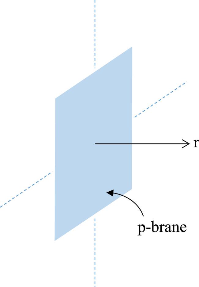
Figure 5. 1/2 BPS p-brane configuration. |
Given what has been said, for a coupled system of a p-brane and the background fields involving gravity, finding a static SUSY-preserving 1/2 BPS p-brane vacuum-like configuration is not so obvious at first glance partly because of the higher non-linearity of the system (unlike the case of finding the electric field of a given charge from the linear Maxwell equations in four dimensions). Nevertheless, the physical basis we gave earlier implies the existence of such an SUSY-preserving configuration. Once such a brane source is placed in spacetime, we expect the original underlying symmetry PD to be broken to Pd × SO(D-d) with d=1+p and Pd being the d-dimensional Poincaré group. If we split the D-coordinates as xM=(xμ, xm) with μ=0, 1, ⋯ p and m=d, d+1, ⋯ D-1. Therefore, we have the most general ansatz for the D-dimensional Einstein frame metric, respecting this residue symmetry, as
$\begin{eqnarray}{\rm{d}}{s}^{2}={{\rm{e}}}^{2A(r)}{\eta }_{\mu \nu }{\rm{d}}{x}^{\mu }{\rm{d}}{x}^{\nu }+{{\rm{e}}}^{2B(r)}{\delta }_{mn}{\rm{d}}{x}^{m}{\rm{d}}{x}^{n},\end{eqnarray}$
with $r=\sqrt{{\delta }_{mn}{x}^{m}{x}^{n}}$ the radial coordinate along the transverse directions of the brane.The ansatz for the dilaton Φ is Φ=Φ(r). If the brane is treated as an electric-like source, then the ansatz for the (1 + p)-form potential is
$\begin{eqnarray}{A}_{01\cdots p}=-\left({{\rm{e}}}^{C(r)}-1\right).\end{eqnarray}$
As described above, we are looking for the static field configuration produced by the brane source, which is also static, and the whole system preserves a certain amount of SUSY (here actually 1/2). For this reason, the worldvolume fields of the brane are all frozen except for the embedding coordinates describing the location of the brane. For the infinitely extended brane, we expect to have $\begin{eqnarray}{\sigma }^{\mu }={X}^{\mu },\qquad {X}^{m}=0,\end{eqnarray}$
i.e., the brane is located at r=0 along the directions transverse to the brane.Since the brane configuration along with the source is invariant under Pd × SO(D-d) and this is a vacuum-like configuration, the spacetime (bulk) fermionic fields and the worldvolume fermionic fields must be both set to vanish. In other words, only the relevant bosonic fields, which remain invariant under the residue symmetry Pd × SO(D-d), are relevant to this configuration.
This configuration is expected to preserve some SUSY; therefore, the transformations of both the bosonic fields and the fermionic fields are also expected to vanish such that this configuration remains invariant under the unbroken SUSY.
As will be seen, this remains true automatically for the bosonic fields once the fermionic ones are set to vanish and the requirement that the transformed fermionic fields remain so determines how many SUSYs are preserved for this configuration.
3.2. p-branes in diverse dimensions
Given that the fermionic fields for both bulk and worldvolume are set to vanish, we need only to consider the relevant bosonic fields8 in the corresponding supergravity action plus the bosonic action of the brane. In other words, we only need to consider the bosonic action of the combined bulk and brane, i.e., ID(d)+Sd, where the Einstein-frame bulk action is
$\begin{eqnarray}\begin{array}{rcl}{I}_{D}(d) & =& \displaystyle \frac{1}{2{\kappa }^{2}}\int {{\rm{d}}}^{D}x\sqrt{-g}\left(R-\displaystyle \frac{1}{2}{(\partial \bar{\phi })}^{2}\right.\\ & & \left.-\,\displaystyle \frac{1}{2(d+1)!}{{\rm{e}}}^{-\alpha (d)\bar{\phi }}{F}_{d+1}^{2}\right)\end{array}\end{eqnarray}$
and the brane sigma-model one is $\begin{eqnarray}\begin{array}{rcl}{S}_{d} & =& {T}_{p}\displaystyle \int {{\rm{d}}}^{d}\sigma \left[-\frac{1}{2}\sqrt{-h}\,{h}^{\alpha \beta }{\partial }_{\alpha }{X}^{M}{\partial }_{\beta }{X}^{N}{G}_{MN}+\frac{d-2}{2}\sqrt{-h}\right.\\ & & -\,\left.\frac{1}{d!}{\epsilon }^{{\alpha }_{1}\cdots {\alpha }_{d}}{\partial }_{{\alpha }_{1}}{X}^{{M}_{1}}\cdots {\partial }_{{\alpha }_{d}}{X}^{{M}_{d}}{A}_{{M}_{1}\cdots {M}_{d}}\right].\end{array}\end{eqnarray}$
In the above, both the p-brane σ-model metric GMN and the Einstein metric gMN are asymptotically flat and the possible vacuum expectation value of Φ or its asymptotically one is absorbed into the respective factors. So the κ and the brane tension Tp are both physical.In the above, Fd+1=dAd, d=p+1 and the p-brane frame metric ${G}_{MN}={g}_{MN}{{\rm{e}}}^{\alpha (d)\bar{\phi }/d}$ with gMN the Einstein frame metric (See [31] for deriving this relation) and $\bar{\phi }=\phi -{\phi }_{0}$ with ⟨Φ⟩=Φ0 and the string coupling ${g}_{s}={{\rm{e}}}^{{\phi }_{0}}$. We have also the following: For D=11, α(d)=0; For D=10, if we choose to relate the relevant parameters to string ones, we have $2{\kappa }^{2}={(2\pi )}^{7}{\alpha }^{{}^{{\prime} }4}{g}_{s}^{2}$ and
$\begin{eqnarray}\begin{array}{rcl}\alpha (d) & =& \displaystyle \frac{3-p}{2}\,(\mathrm{NS(NS)}\,p-\mathrm{brane}),\\ \alpha (d) & =& \displaystyle \frac{p-3}{2}\,({Dp}-\mathrm{brane}),\\ {T}_{{\rm{F}}} & =& \displaystyle \frac{1}{2\pi {\alpha }^{{}^{^{\prime} }}},\quad {T}_{\mathrm{NS\; 5}}=\displaystyle \frac{1}{{g}_{s}^{2}{(2\pi )}^{5}{\alpha }^{{}^{^{\prime} }3}},\\ {T}_{\mathrm{Dp}} & =& \displaystyle \frac{1}{{g}_{s}{(2\pi )}^{p}{\alpha }^{{}^{^{\prime} }(1+p)/2}}.\end{array}\end{eqnarray}$
For a 1/2 BPS p-brane in diverse dimensions with the corresponding supergravity having a maximal SUSY, we have in general9 $\begin{eqnarray}{\alpha }^{2}(d)=4-\frac{2d\tilde{d}}{D-2},\end{eqnarray}$
with $\tilde{d}=D-2-d$.From the action ID(d)+Sd with ID(d) given in (30 ) and Sd given in (31 ), the EOMs are, for the metric 27 ). So 37 ) is now 28 ), we have 34 ) are
$\begin{eqnarray}\begin{array}{rcl} & & {R}_{MN}-\displaystyle \frac{1}{2}{g}_{MN}R-\displaystyle \frac{1}{2}\left({\partial }_{M}\bar{\phi }{\partial }_{N}\bar{\phi }-\displaystyle \frac{1}{2}{g}_{MN}{(\partial \bar{\phi })}^{2}\right)\\ & & \quad -\displaystyle \frac{1}{2d!}\left({F}_{M{M}_{1}\cdots {M}_{d}}{F}_{N}{\,}^{{M}_{1}\cdots {M}_{d}}\right.\\ & & \quad \left.-\displaystyle \frac{1}{2(d+1)}{g}_{MN}{F}_{d+1}^{2}\right){{\rm{e}}}^{-\alpha (d)\bar{\phi }}={\kappa }^{2}{T}_{MN}(p-\mathrm{brane}),\end{array}\end{eqnarray}$
for the dilaton $\begin{eqnarray}\begin{array}{rcl} & & {\partial }_{M}(\sqrt{-g}{g}^{MN}{\partial }_{N}\bar{\phi })+\frac{\alpha (d)}{2(d+1)!}\sqrt{-g}{{\rm{e}}}^{-\alpha (d)\bar{\phi }}{F}_{d+1}^{2}\\ & & \quad =\frac{\alpha (d){\kappa }^{2}{T}_{p}}{d}\displaystyle \int {{\rm{d}}}^{d}\sigma \sqrt{-h}\,{h}^{\alpha \beta }\\ & & \quad \times \,{\partial }_{\alpha }{X}^{M}{\partial }_{\beta }{X}^{N}{g}_{MN}{{\rm{e}}}^{\alpha (d)\bar{\phi }/d}{\delta }^{(D)}(x-X),\end{array}\end{eqnarray}$
and for the d-form potential $\begin{eqnarray}\begin{array}{rcl} & & {\partial }_{M}\left(\sqrt{-g}{{\rm{e}}}^{-\alpha (d)\bar{\phi }}{F}^{M{M}_{1}\cdots {M}_{d}}\right)\\ & & \quad =2{\kappa }^{2}{T}_{p}\displaystyle \int {{\rm{d}}}^{d}\sigma {\epsilon }^{{\alpha }_{1}\cdots {\alpha }_{d}}{\partial }_{{\alpha }_{1}}{X}^{{M}_{1}}\cdots {\partial }_{{\alpha }_{d}}{X}^{{M}_{d}}{\delta }^{(D)}(x-X).\end{array}\end{eqnarray}$
In the above, the energy-momentum tensor with up indices is $\begin{eqnarray}\begin{array}{rcl} & & {T}^{MN}({\rm{p}}-\mathrm{brane})\\ & & \quad =-{T}_{p}\int {{\rm{d}}}^{d}\sigma \sqrt{-h}\,{h}^{\alpha \beta }{\partial }_{\alpha }{X}^{M}{\partial }_{\beta }{X}^{N}{{\rm{e}}}^{\alpha (d)\bar{\phi }/d}\displaystyle \frac{{\delta }^{(D)}(x-X)}{\sqrt{-g}}.\end{array}\end{eqnarray}$
The p-brane EOMs are, for XM $\begin{eqnarray}\begin{array}{rcl} & & {\partial }_{\alpha }\left(\sqrt{-h}\,{h}^{\alpha \beta }{\partial }_{\beta }{X}^{N}{g}_{MN}{{\rm{e}}}^{\alpha (d)\bar{\phi }/d}\right)\\ & & \quad -\frac{1}{2}\sqrt{-h}\,{h}^{\alpha \beta }{\partial }_{\alpha }{X}^{N}{\partial }_{\beta }{X}^{P}{\partial }_{M}\left({g}_{NP}{{\rm{e}}}^{\alpha (d)\bar{\phi }/d}\right)\\ & & -\frac{1}{d!}{\epsilon }^{{\alpha }_{1}\cdots {\alpha }_{d}}{\partial }_{{\alpha }_{1}}{X}^{{M}_{1}}\cdots {\partial }_{{\alpha }_{d}}{X}^{{M}_{d}}{F}_{M{M}_{1}\cdots {M}_{d}}=0,\end{array}\end{eqnarray}$
and for the worldvolume metric hαβ $\begin{eqnarray}{h}_{\alpha \beta }={\partial }_{\alpha }{X}^{M}{\partial }_{\beta }{X}^{N}{g}_{MN}{{\rm{e}}}^{\alpha (d)\bar{\phi }/d}.\end{eqnarray}$
For a static p-brane (Xμ=σμ, Xm=0), we have $\begin{eqnarray}{h}_{\mu \nu }={g}_{\mu \nu }{{\rm{e}}}^{\alpha (d)\bar{\phi }/d}={\eta }_{\mu \nu }{{\rm{e}}}^{2A+\alpha (d)\bar{\phi }/d},\end{eqnarray}$
where μ, ν=0, 1, ⋯ p and the metric gMN is given by ( $\begin{eqnarray}h=\det {h}_{\mu \nu }=-{{\rm{e}}}^{2Ad+\alpha (d)\bar{\phi }},\quad g=\det {g}_{MN}=-{{\rm{e}}}^{2Ad+2B(D-d)}.\end{eqnarray}$
The energy-momentum tensor ( $\begin{eqnarray}\begin{array}{rcl}{T}_{\mu \nu } & =& -{T}_{p}\,{\eta }_{\mu \nu }\,{{\rm{e}}}^{2A-B(D-d)+\alpha (d)\bar{\phi }/2}\,{\delta }^{(D-d)}({x}_{\perp }),\\ {T}_{mn} & =& 0.\end{array}\end{eqnarray}$
From ( $\begin{eqnarray}\begin{array}{rcl} & & {F}_{\mu {M}_{1}\cdots {M}_{d}}{F}_{\nu }{\,}^{{M}_{1}\cdots {M}_{d}}\\ & & \quad =-d!\,{\eta }_{\mu \nu }{{\rm{e}}}^{-2A(d-1)-2B+2C}{\delta }^{mn}{\partial }_{m}C{\partial }_{n}C,\\ & & \quad {F}_{m{M}_{1}\cdots {M}_{d}}{F}_{n}{\,}^{{M}_{1}\cdots {M}_{d}}\\ & & \quad =-d!\,{{\rm{e}}}^{-2Ad+2C}\,{\partial }_{m}C{\partial }_{n}C,\\ & & {F}_{d+1}^{2}\\ & & \quad =-(d+1)!\,{{\rm{e}}}^{-2B-2Ad+2C}\,{\delta }^{mn}{\partial }_{m}C{\partial }_{n}C.\end{array}\end{eqnarray}$
With the given ansatz, the μν-components of the Einstein EOM ( $\begin{eqnarray}\begin{array}{l}{\delta }^{mn}\left[\Space{0ex}{3ex}{0ex}(d-1){\partial }_{m}{\partial }_{n}A+(\tilde{d}+1){\partial }_{m}{\partial }_{n}B\right.\\ \quad +\tilde{d}(d-1){\partial }_{m}A{\partial }_{n}B\\ \quad +\frac{d(d-1)}{2}{\partial }_{m}A{\partial }_{n}A+\frac{\tilde{d}(\tilde{d}+1)}{2}{\partial }_{m}B{\partial }_{n}B\\ \quad +\frac{1}{4}{\partial }_{m}\bar{\phi }{\partial }_{n}\bar{\phi }\\ \left.\quad +\frac{1}{4}{{\rm{e}}}^{-2dA+2C-\alpha (d)\bar{\phi }}{\partial }_{m}C{\partial }_{n}C\right]\\ \quad =-{\kappa }^{2}{T}_{p}{{\rm{e}}}^{-B\tilde{d}+\alpha (d)\bar{\phi }/2}{\delta }^{(D-d)}({x}_{\perp }),\end{array}\end{eqnarray}$
and the mn-components $\begin{eqnarray}\begin{array}{l}-\tilde{d}\left({\partial }_{m}{\partial }_{n}B-{\delta }_{mn}{\delta }^{kl}{\partial }_{k}{\partial }_{l}B\right)-d\left({\partial }_{m}{\partial }_{n}A-{\delta }_{mn}{\delta }^{kl}{\partial }_{k}{\partial }_{l}A\right)\\ \quad -d\left({\partial }_{m}A{\partial }_{n}A-\frac{d+1}{2}{\delta }_{mn}{\delta }^{kl}{\partial }_{k}A{\partial }_{l}A\right)\\ \quad +\tilde{d}\left({\partial }_{m}B{\partial }_{n}B+\frac{\tilde{d}-1}{2}{\delta }_{mn}{\delta }^{kl}{\partial }_{k}B{\partial }_{l}B\right)\\ \quad +d\left({\partial }_{m}A{\partial }_{n}B+{\partial }_{m}B{\partial }_{n}A+(\tilde{d}-1){\delta }_{mn}{\delta }^{kl}{\partial }_{k}A{\partial }_{l}B\right)\\ \quad -\frac{1}{2}{\partial }_{m}\bar{\phi }{\partial }_{n}\bar{\phi }+\frac{1}{4}{\delta }_{mn}{\delta }^{kl}{\partial }_{k}\bar{\phi }{\partial }_{l}\bar{\phi }\\ \quad -\frac{1}{2}{{\rm{e}}}^{-2dA+2C-\alpha (d)\bar{\phi }}\left[-{\partial }_{m}C{\partial }_{n}C+\frac{1}{2}{\delta }_{mn}{\delta }^{kl}{\partial }_{k}C{\partial }_{l}C\right]=0,\end{array}\end{eqnarray}$
which can be rewritten as $\begin{eqnarray}\begin{array}{l}-{\partial }_{m}{\partial }_{n}(dA+\tilde{d}B)+{\partial }_{m}(dA+\tilde{d}B){\partial }_{n}B\\ \quad +d{\partial }_{m}(B-A){\partial }_{n}A-\frac{1}{2}{\partial }_{m}\bar{\phi }{\partial }_{n}\bar{\phi }\\ \quad +\frac{1}{2}{{\rm{e}}}^{-2dA+2C-\alpha \bar{\phi }}{\partial }_{m}C{\partial }_{n}C\\ \quad +{\delta }_{mn}{\delta }^{kl}\left[{\partial }_{k}{\partial }_{l}(dA+\tilde{d}B)+d(\tilde{d}-1){\partial }_{k}A{\partial }_{l}B\right.\\ \quad +\frac{d(d+1)}{2}{\partial }_{k}A{\partial }_{l}A+\frac{\tilde{d}(\tilde{d}-1)}{2}{\partial }_{k}B{\partial }_{l}B\\ \quad \left.+\frac{1}{4}{\partial }_{k}\bar{\phi }{\partial }_{l}\bar{\phi }-\frac{1}{4}{{\rm{e}}}^{-2dA+2C-\alpha \bar{\phi }}{\partial }_{k}C{\partial }_{l}C\right]=0.\end{array}\end{eqnarray}$
In deriving the above two equations, given the metric form, $\begin{eqnarray}{\rm{d}}{s}^{2}={{\rm{e}}}^{2A(r)}{\eta }_{\mu \nu }{\rm{d}}{x}^{\mu }{\rm{d}}{x}^{\nu }+{{\rm{e}}}^{2B(r)}{\delta }_{mn}{\rm{d}}{y}^{m}{\rm{d}}{y}^{n},\end{eqnarray}$
with μ, ν=0, 1, ⋯ d-1 and m, n=d, ⋯ D-1, we have used the following $\begin{eqnarray}{R}_{\mu \nu }=-{\eta }_{\mu \nu }{{\rm{e}}}^{2(A-B)}{\delta }^{mn}\left({\partial }_{m}{\partial }_{n}A+d\,{\partial }_{m}A{\partial }_{n}A+\tilde{d}\,{\partial }_{m}A{\partial }_{n}B\right),\end{eqnarray}$
$\begin{eqnarray}\begin{array}{rcl}{R}_{mn} & =& -\tilde{d}\,{\partial }_{m}{\partial }_{n}B-{\delta }_{mn}{\delta }^{kl}{\partial }_{k}{\partial }_{l}B\\ & & -d\,{\partial }_{m}{\partial }_{n}A-d\,{\partial }_{m}A{\partial }_{n}A\\ & & +d\left({\partial }_{m}A{\partial }_{n}B+{\partial }_{m}B{\partial }_{n}A-{\delta }_{mn}{\delta }^{kl}{\partial }_{k}A{\partial }_{l}B\right)\\ & & +\tilde{d}\left({\partial }_{m}B{\partial }_{n}B-{\delta }_{mn}{\delta }^{kl}{\partial }_{k}B{\partial }_{l}B\right),\end{array}\end{eqnarray}$
$\begin{eqnarray}\begin{array}{rcl}R & =& -{{\rm{e}}}^{-2B}{\delta }^{kl}\left[2\,d\,{\partial }_{k}{\partial }_{l}A+d(d+1)\,{\partial }_{k}A{\partial }_{l}A\right.\\ & & +2\,d\,\tilde{d}\,{\partial }_{k}A{\partial }_{l}B+2\,(\tilde{d}+1)\,{\partial }_{k}{\partial }_{l}B\\ & & \left.+\tilde{d}\,(\tilde{d}+1){\partial }_{k}B{\partial }_{l}B\right].\end{array}\end{eqnarray}$
In the above, $\tilde{d}=D-d-2$.The EOM for the dilaton (35 ) reduces to 36 ) reduces to 38 ) now becomes
$\begin{eqnarray}\begin{array}{rcl} & & {\delta }^{mn}{\partial }_{m}\left({{\rm{e}}}^{Ad+B\tilde{d}}{\partial }_{n}\bar{\phi }\right)-\frac{\alpha (d)}{2}{{\rm{e}}}^{B\tilde{d}-Ad-\alpha (d)\bar{\phi }+2C}{\delta }^{mn}{\partial }_{m}C{\partial }_{n}C\\ & & \,=\alpha (d)\,{\kappa }^{2}\,{T}_{p}\,{{\rm{e}}}^{Ad+\alpha (d)\bar{\phi }/2}{\delta }^{(D-d)}({x}_{\perp }),\end{array}\end{eqnarray}$
and the EOM for the d-form potential ( $\begin{eqnarray}{\delta }^{mn}{\partial }_{m}\left({{\rm{e}}}^{B\tilde{d}-Ad-\alpha (d)\bar{\phi }+2C}{\partial }_{n}{{\rm{e}}}^{-C}\right)=-2\,{\kappa }^{2}\,{T}_{p}\,{\delta }^{(D-d)}({x}_{\perp }),\end{eqnarray}$
and the EOM for the p-brane ( $\begin{eqnarray}{\partial }_{m}\left({{\rm{e}}}^{C}-{{\rm{e}}}^{Ad+\alpha (d)\bar{\phi }/2}\right)=0,\end{eqnarray}$
which is usually called the ‘no force' condition.Note that $A(r\to \infty )=B(r\to \infty )=\bar{\phi }(r\to \infty )=0$. If we choose C(r →∞)=0 (a proper choice for which A01⋯p(r →∞) →0), then from the last equation, we have 52 ) 51 ) and combined with the above, we have 54 ) and (33 ). Note that here A, B, C, Φ are the functions of variable r only, so we have 44 ), using (55 ) to replace the Δ-function on the right, can be rewritten as 54 ) to replace $\bar{\phi }$ by A and C. This can be further rewritten as 46 ), we have 54 ) to replace $\bar{\phi }$ in terms of A and C. The m=n components of (46 ) give 62 ) from (60 ) to give 57 ) can also be expressed as 63 ) and (64 ) gives 64 ) and (65 ) to give 61 ) from 2 × (62 ) to give 54 ), when combined with the other EOMs, already imply the preservation of 1/2 SUSY. The ‘no-force' condition (54 ) plays the key role here. We will see later that, when this condition is dropped, we can find so-called non-SUSY brane solutions.
$\begin{eqnarray}C=Ad+\alpha (d)\bar{\phi }/2.\end{eqnarray}$
With this, we have from ( $\begin{eqnarray}{\delta }^{mn}{\partial }_{m}\left({{\rm{e}}}^{dA+\tilde{d}B}{\partial }_{n}{{\rm{e}}}^{-C}\right)=-2{\kappa }^{2}{T}_{p}\,{\delta }^{(D-d)}({x}_{\perp }).\end{eqnarray}$
From ( $\begin{eqnarray}{\delta }^{mn}{\partial }_{m}\left[{{\rm{e}}}^{dA+\tilde{d}B}{\partial }_{n}\left(C-\frac{2\bar{\phi }}{\alpha (d)}\right)\right]=0,\end{eqnarray}$
or $\begin{eqnarray}{\delta }^{mn}{\partial }_{m}\left[{{\rm{e}}}^{dA+\tilde{d}B}{\partial }_{n}\left(A-\frac{\tilde{d}}{2(d+\tilde{d})}C\right)\right]=0,\end{eqnarray}$
where we have used ( $\begin{eqnarray}\begin{array}{l}{\delta }^{mn}{\partial }_{m}\left({{\rm{e}}}^{dA+\tilde{d}B}{\partial }_{n}F(r)\right)\\ \quad ={{\rm{e}}}^{dA+\tilde{B}}\left({F}^{{\prime\prime} }+\frac{\tilde{d}+1}{r}{F}^{{\prime} }+{(dA+\tilde{d}B)}^{{\prime} }{F}^{{\prime} }\right),\\ \quad {\delta }^{mn}{\partial }_{m}{\partial }_{n}F={F}^{{\prime\prime} }+\frac{\tilde{d}+1}{r}{F}^{{\prime} },\end{array}\end{eqnarray}$
where ${F}^{{\prime} }\equiv {\rm{d}}F/{\rm{d}}r,{F}^{{\prime\prime} }\equiv {{\rm{d}}}^{2}F/{\rm{d}}{r}^{2}$. Then the EOM ( $\begin{eqnarray}\begin{array}{rcl}0 & =& {(dA+\tilde{d}B)}^{{\prime\prime} }+\frac{\tilde{d}+1}{r}{(dA+\tilde{d}B)}^{{\prime} }\\ & & +\frac{1}{2}{(dA+\tilde{d}B)}^{{}^{{\prime} }2}-\frac{1}{2}{A}^{{\prime} }{(dA+\tilde{d}B)}^{{\prime} }\\ & & -{(A-B)}^{{\prime\prime} }-\frac{\tilde{d}+1}{r}{(A-B)}^{{\prime} }-\frac{\tilde{d}}{2}{(A-B)}^{{\prime} }{B}^{{\prime} }\\ & & +\frac{1}{2}\left({C}^{{\prime\prime} }+\frac{\tilde{d}+1}{r}{C}^{{\prime} }\right)\\ & & -\frac{d{C}^{{\prime} }}{{\alpha }^{2}}{\left(A-\frac{\tilde{d}}{2(d+\tilde{d})}C\right)}^{{\prime} }+\frac{d{A}^{{\prime} }}{{\alpha }^{2}}{(dA-C)}^{{\prime} }\\ & & +\frac{1}{2}{\left(dA+\tilde{d}B\right)}^{{\prime} }{C}^{{\prime} },\end{array}\end{eqnarray}$
where we have used ( $\begin{eqnarray}\begin{array}{l}{\left(B-A+\frac{C}{2}\right)}^{{\prime\prime} }+\frac{\tilde{d}+1}{r}{\left(B-A+\frac{C}{2}\right)}^{{\prime} }\\ \quad +\frac{\tilde{d}}{2}{B}^{{\prime} }{\left(B-A+\frac{C}{2}\right)}^{{\prime} }\\ \quad +{(dA+\tilde{d}B)}^{{\prime\prime} }+\frac{\tilde{d}+1}{r}{(dA+\tilde{d}B)}^{{\prime} }+\frac{1}{2}{(dA+\tilde{d}B)}^{{}^{{\prime} }2}\\ \quad -\frac{1}{2}{\left(A-\frac{C}{2}\right)}^{{\prime} }{(dA+\tilde{d}B)}^{{\prime} }\\ \quad +\frac{d}{{\alpha }^{2}}{(dA-C)}^{{\prime} }{\left(A-\frac{\tilde{d}}{2(d+\tilde{d})}C\right)}^{{\prime} }=0.\end{array}\end{eqnarray}$
For the m ≠ n components of ( $\begin{eqnarray}\begin{array}{l}{(dA+\tilde{d}B)}^{{\prime\prime} }-\frac{1}{r}{(dA+\tilde{d}B)}^{{\prime} }\\ \quad -{B}^{{\prime} }{\left(dA+\tilde{d}B\right)}^{{\prime} }-d{A}^{{\prime} }{\left(B-A+\frac{C}{2}\right)}^{{\prime} }\\ \quad +\frac{2d}{{\alpha }^{2}}{\left(dA-C\right)}^{{\prime} }{\left(A-\frac{\tilde{d}}{2(d+\tilde{d})}C\right)}^{{\prime} }=0,\end{array}\end{eqnarray}$
where we also use ( $\begin{eqnarray}\begin{array}{r}{(dA+\tilde{d}B)}^{{\prime\prime} }+\frac{\tilde{d}+1}{r}{(dA+\tilde{d}B)}^{{\prime} }\\ \quad +\frac{1}{2}{(dA+\tilde{d}B)}^{{}^{{\prime} }2}-\frac{1}{2}{B}^{{\prime} }{(dA+\tilde{d}B)}^{{\prime} }\\ \quad -\frac{d}{2}{A}^{{\prime} }{\left(B-A+\frac{C}{2}\right)}^{{\prime} }+\frac{d}{{\alpha }^{2}}{(dA-C)}^{{\prime} }\\ \quad \times {\left(A-\frac{\tilde{d}}{2(d+\tilde{d})}C\right)}^{{\prime} }=0.\end{array}\end{eqnarray}$
We subtract ( $\begin{eqnarray}\begin{array}{l}{\left(B-A+\frac{C}{2}\right)}^{{\prime\prime} }+\frac{\tilde{d}+1}{r}{\left(B-A+\frac{C}{2}\right)}^{{\prime} }\\ \quad +{(dA+\tilde{d}B)}^{{\prime} }\left(B-A+\frac{C}{2}\right)=0.\end{array}\end{eqnarray}$
The EOM ( $\begin{eqnarray}\begin{array}{l}{\left(A-\frac{\tilde{d}}{2(d+\tilde{d})}C\right)}^{{\prime\prime} }+\frac{\tilde{d}+1}{r}{\left(A-\frac{\tilde{d}}{2(d+\tilde{d})}C\right)}^{{\prime} }\\ \quad +{(dA+\tilde{d}B)}^{{\prime} }{\left(A-\frac{\tilde{d}}{2(d+\tilde{d})}C\right)}^{{\prime} }=0.\end{array}\end{eqnarray}$
Combining ( $\begin{eqnarray}\begin{array}{r}{\left(B+\frac{d}{2(d+\tilde{d})}C\right)}^{{\prime\prime} }+\frac{\tilde{d}+1}{r}{\left(B+\frac{d}{2(d+\tilde{d})}C\right)}^{{\prime} }\\ \quad +{(dA+\tilde{d}B)}^{{\prime} }{\left(B+\frac{d}{2(d+\tilde{d})}C\right)}^{{\prime} }=0.\end{array}\end{eqnarray}$
We further combine ( $\begin{eqnarray}{\left(dA+\tilde{d}B\right)}^{{\prime\prime} }+\frac{\tilde{d}+1}{r}{\left(dA+\tilde{d}B\right)}^{{\prime} }+{{(dA+\tilde{d}B)}^{{\prime} }}^{2}=0.\end{eqnarray}$
We subtract ( $\begin{eqnarray}{\left(dA+\tilde{d}B\right)}^{{\prime\prime} }+\frac{2\tilde{d}+3}{r}{\left(dA+\tilde{d}B\right)}^{{\prime} }+{{(dA+\tilde{d}B)}^{{\prime} }}^{2}=0.\end{eqnarray}$
The above two equations must imply $\begin{eqnarray}{(dA+\tilde{d}B)}^{{\prime} }=0,\end{eqnarray}$
which in turn gives, noting A(r →∞)=0, B(r →∞)=0, $\begin{eqnarray}dA+\tilde{d}B=0.\end{eqnarray}$
As we will demonstrate, this condition and the so-called ‘no-force' condition (With this, we have from (61 ) the non-trivial solution 69 ), this gives also
$\begin{eqnarray}{\left(A-\frac{\tilde{d}}{2(d+\tilde{d})}C\right)}^{{\prime} }=0,\end{eqnarray}$
which gives $\begin{eqnarray}A=\frac{\tilde{d}}{2(d+\tilde{d})}C,\end{eqnarray}$
due to A(r →∞)=C(r →∞)=0. So with ( $\begin{eqnarray}B=-\frac{d}{2(d+\tilde{d})}C.\end{eqnarray}$
One can check that the following 60 ), (61 ), (62 ) and (64 ). So we have also from (54 ) 55 ), to
$\begin{eqnarray}A=\frac{\tilde{d}}{2(d+\tilde{d})}C,\quad B=-\frac{d}{2(d+\tilde{d})}C\end{eqnarray}$
solve all equations ( $\begin{eqnarray}\bar{\phi }=\frac{\alpha }{2}C.\end{eqnarray}$
In other words, all the EOMs boil down, from ( $\begin{eqnarray}{\delta }^{mn}{\partial }_{m}{\partial }_{n}{{\rm{e}}}^{-C}=-2{\kappa }^{2}{T}_{p}\,{\delta }^{(D-d)}({x}_{\perp }),\end{eqnarray}$
which gives the solution $\begin{eqnarray}{{\rm{e}}}^{-C}=1+\frac{{K}_{d}}{{r}^{\tilde{d}}},\end{eqnarray}$
where $\begin{eqnarray}{K}_{d}=\frac{2{\kappa }^{2}{T}_{p}}{\tilde{d}\,{{\rm{\Omega }}}_{\tilde{d}+1}},\quad {{\rm{\Omega }}}_{n}=\frac{2{\pi }^{(n+1)/2}}{{\rm{\Gamma }}((n+1)/2)},\end{eqnarray}$
with Ωn the volume of unity n-sphere.In summary, we find the SUSY-preserving configurations in diverse dimensions with $\tilde{d}=D-2-d\,\geqslant \,1\to D\,\geqslant \,3+d\,\geqslant \,4$ due to d ≥ 1 as
$\begin{eqnarray}{\rm{d}}{s}^{2}={{\rm{e}}}^{\frac{\tilde{d}}{D-2}C}{\eta }_{\mu \nu }{\rm{d}}{x}^{\mu }{\rm{d}}{x}^{\nu }+{{\rm{e}}}^{-\frac{d}{D-2}C}{\delta }_{mn}{\rm{d}}{x}^{m}{\rm{d}}{x}^{n},\end{eqnarray}$
where μ, ν=0, 1 ⋯ p and m, n=p+1, …D-1, $\begin{eqnarray}{A}_{01\cdots p}=-\left({{\rm{e}}}^{C}-1\right),\quad \bar{\phi }=\frac{\alpha }{2}C,\end{eqnarray}$
and $\begin{eqnarray}{{\rm{e}}}^{-C}=1+\frac{{K}_{d}}{{r}^{\tilde{d}}},\end{eqnarray}$
where $\begin{eqnarray}{K}_{d}=\frac{2{\kappa }^{2}{T}_{p}}{\tilde{d}\,{{\rm{\Omega }}}_{\tilde{d}+1}},\quad {{\rm{\Omega }}}_{n}=\frac{2{\pi }^{(n+1)/2}}{{\rm{\Gamma }}((n+1)/2)},\end{eqnarray}$
with Ωn the volume of unity n-sphere.3.3. Certain properties of the solutions
The charge density carried by a p-brane moving in spacetime is given by (22 ) as
$\begin{eqnarray}\begin{array}{l}{j}^{{M}_{1}\cdots {M}_{p+1}}(x)={T}_{p}\displaystyle \int {{\rm{d}}}^{p+1}\sigma {\epsilon }^{{i}_{1}\cdots {i}_{p+1}}{\partial }_{{i}_{1}}\\ \quad \times {X}^{{M}_{1}}\cdots {\partial }_{{i}_{p+1}}{X}^{{M}_{p+1}}{\delta }^{(D)}\left(x-X(\sigma )\right),\end{array}\end{eqnarray}$
where we have taken the charge density μp=Tp. For a static p-brane with σμ=Xμ, we have the familiar one $\begin{eqnarray}{j}^{01\cdots p}(x)={T}_{p}\,{\delta }^{(D-p-1)}({x}_{\perp }),\end{eqnarray}$
and the total charge carried by the brane is $\begin{eqnarray}{Z}^{1\cdots p}=\int {{\rm{d}}}^{D-1}x\,{j}^{01\cdots p}(x)={T}_{p}\,{V}_{p},\end{eqnarray}$
which gives the charge density as Z1⋯p/Vp=Tp. In general, the current density ${j}^{{M}_{1}\cdots {M}_{p+1}}$ is a (p + 1)-form.The EOM for the (p + 1)-form potential Ad as given in (36 ) can be expressed in terms of ${j}^{{M}_{1}\cdots {M}_{p+1}}$ as 85 ) and Jd used in the last equality is a tensor defined as
$\begin{eqnarray}{\partial }_{M}\left(\sqrt{-g}{{\rm{e}}}^{-\alpha (d)\bar{\phi }}{F}^{M{M}_{1}\cdots {M}_{d}}\right)=2{\kappa }^{2}{j}^{{M}_{1}\cdots {M}_{d}}\end{eqnarray}$
and the Bianchi identity is simply ${\partial }_{\left[{M}_{1}\right.}{F}_{{M}_{2}\cdots {M}_{d+2}\left.\right]}=0$. Note that $\begin{eqnarray}\begin{array}{l}{\rm{d}}* \left({{\rm{e}}}^{-\alpha \bar{\phi }}{F}_{d+1}\right)\\ \quad =\frac{1}{(D-d-1)!}{\partial }_{M}* {\left({{\rm{e}}}^{-\alpha \bar{\phi }}F\right)}_{{M}_{d+2}\cdots {M}_{D}}{\rm{d}}{x}^{M}\\ \,\times \wedge {\rm{d}}{x}^{{M}_{d+2}}\cdots \wedge {\rm{d}}{x}^{{M}_{D}}\\ \quad =\frac{{\varepsilon }_{{M}_{d+2}\cdots {M}_{D}{M}_{1}\cdots {M}_{d+1}}}{(D-d-1)!(d+1)!}{\partial }_{M}\left[\sqrt{| g| }{{\rm{e}}}^{-\alpha \bar{\phi }}{F}^{{M}_{1}\cdots {M}_{d+1}}\right]\\ \,\times {\delta }_{{N}_{1}{N}_{2}\cdots {N}_{D-d}}^{M{M}_{d+2}\cdots {M}_{D}}{\rm{d}}{x}^{{N}_{1}}\wedge {\rm{d}}{x}^{{N}_{2}}\cdots \wedge {\rm{d}}{x}^{{N}_{D-d}}\\ \quad =\frac{{\varepsilon }_{{M}_{d+2}\cdots {M}_{D}{M}_{1}\cdots {M}_{d+1}}}{(D-d-1)!(d+1)!}{\partial }_{M}\left[\sqrt{| g| }{{\rm{e}}}^{-\alpha \bar{\phi }}{F}^{{M}_{1}\cdots {M}_{d+1}}\right]\\ \,\times \,\frac{{(-)}^{t}}{(D-d)!d!}\times {\epsilon }^{M{M}_{d+2}\cdots {M}_{D}{L}_{1}\cdots {L}_{d}}{\epsilon }_{{N}_{1}{N}_{2}\cdots {N}_{D-d}{L}_{1}\cdots {L}_{d}}{\rm{d}}{x}^{{N}_{1}}\\ \,\times \wedge {\rm{d}}{x}^{{N}_{2}}\cdots {\rm{d}}{x}^{{N}_{D-d}}\\ \quad =\frac{{(-)}^{D-d-1}{\delta }_{{M}_{1}{M}_{2}\cdots {M}_{d+1}}^{M{L}_{1}\cdots {L}_{d}}}{(D-d)!d!}{\partial }_{M}\left[\sqrt{| g| }{{\rm{e}}}^{-\alpha \bar{\phi }}{F}^{{M}_{1}\cdots {M}_{d+1}}\right]\\ \,\times {\varepsilon }_{{N}_{1}{N}_{2}\cdots {N}_{D-d}{L}_{1}\cdots {L}_{d}}{\rm{d}}{x}^{{N}_{1}}\wedge {\rm{d}}{x}^{{N}_{2}}\cdots {\rm{d}}{x}^{{N}_{D-d}}\\ \quad =\frac{{(-)}^{\tilde{d}+1}}{(D-d)!d!}{\partial }_{M}\left[\sqrt{| g| }{{\rm{e}}}^{-\alpha \bar{\phi }}{F}^{M{L}_{1}\cdots {L}_{d}}\right]{\varepsilon }_{{N}_{1}{N}_{2}\cdots {N}_{D-d}{L}_{1}\cdots {L}_{d}}\\ \,\times {\rm{d}}{x}^{{N}_{1}}\wedge {\rm{d}}{x}^{{N}_{2}}\cdots {\rm{d}}{x}^{{N}_{D-d}}\\ \quad =\frac{{(-)}^{\tilde{d}+1}2{\kappa }^{2}}{(D-d)!d!}{j}^{{L}_{1}\cdots {L}_{d}}{\varepsilon }_{{N}_{1}{N}_{2}\cdots {N}_{D-d}{L}_{1}\cdots {L}_{d}}{\rm{d}}{x}^{{N}_{1}}\\ \,\times \wedge {\rm{d}}{x}^{{N}_{2}}\cdots {\rm{d}}{x}^{{N}_{D-d}}\\ \quad ={(-)}^{\tilde{d}+1}2{\kappa }^{2}* {J}_{d},\end{array}\end{eqnarray}$
where in the second to last equality we have used ( $\begin{eqnarray}{J}_{d}\equiv \frac{1}{d!}\frac{{j}_{{L}_{1}\cdots {L}_{d}}}{\sqrt{| g| }}{\rm{d}}{x}^{{L}_{1}}\wedge \cdots {\rm{d}}{x}^{{L}_{d}}.\end{eqnarray}$
So, writing in terms of differential forms, we have the EOM and Bianchi identity as $\begin{eqnarray}\begin{array}{rcl}{\rm{d}}* \left({{\rm{e}}}^{-\alpha \bar{\phi }}{F}_{d+1}\right) & =& {(-)}^{\tilde{d}+1}2{\kappa }^{2}* {J}_{d},\\ {\rm{d}}{F}_{d+1} & =& 0.\end{array}\end{eqnarray}$
In deriving the above, we have used the following conventions for differential forms and the Hodge duality. We define the totally anti-symmetric symbol ${\varepsilon }^{{i}_{1}\cdots {i}_{D}}$, a tensor density with weight -1, to be the same in all the frames with ϵ1⋯D=1, and define $\begin{eqnarray}{\varepsilon }_{{i}_{1}\cdots {i}_{D}}\equiv {(-)}^{t}{\varepsilon }^{{i}_{1}\cdots {i}_{D}}.\end{eqnarray}$
In the above, we denote t as the number of the negative eigenvalues of the metric gij. We then have two tensors $\begin{eqnarray}{\epsilon }^{{i}_{1}\cdots {i}_{D}}\equiv \frac{{\varepsilon }^{{i}_{1}\cdots {i}_{D}}}{\sqrt{| g| }},\quad {\epsilon }_{{i}_{1}\cdots {i}_{D}}\equiv \sqrt{| g| }{\varepsilon }_{{i}_{1}\cdots {i}_{D}},\end{eqnarray}$
where the upper or lower indices are raised or lowered by the metric or its inverse, and ∣g∣ denotes the absolute value of the metric determinant. We define $\begin{eqnarray}{\epsilon }^{{i}_{1}\cdots {i}_{D}}{\epsilon }_{{j}_{1}\cdots {j}_{D}}=D!{(-)}^{t}{\delta }_{{j}_{1}\cdots {j}_{D}}^{{i}_{1}\cdots {i}_{D}},\end{eqnarray}$
and in general (p+q=D) $\begin{eqnarray}{\epsilon }^{{i}_{1}\cdots {i}_{q}{k}_{1}\cdots {k}_{p}}{\epsilon }_{{j}_{1}\cdots {j}_{q}{k}_{1}\cdots {k}_{p}}=p!q!{(-)}^{t}{\delta }_{{j}_{1}\cdots {j}_{q}}^{{i}_{1}\cdots {i}_{q}},\end{eqnarray}$
$\begin{eqnarray}{\delta }_{{j}_{1}\cdots {j}_{q}}^{{i}_{1}\cdots {i}_{q}}\equiv {\delta }_{\left[{j}_{1}\cdots {j}_{q}\right]}^{\left[{i}_{1}\cdots {i}_{q}\right]}.\end{eqnarray}$
So we have $\begin{eqnarray}{A}_{{i}_{1}\cdots {i}_{p}}{\delta }_{{j}_{1}\cdots {j}_{p}}^{{i}_{1}\cdots {i}_{p}}={A}_{{j}_{1}\cdots {j}_{p}}.\end{eqnarray}$
A p-form is defined $\begin{eqnarray}{\omega }_{p}=\frac{1}{p!}{\omega }_{{i}_{1}\cdots {i}_{p}}{\rm{d}}{x}^{{i}_{1}}\wedge \cdots \wedge {\rm{d}}{x}^{{i}_{p}},\end{eqnarray}$
with the Hodge dual basis $\begin{eqnarray}* \left({\rm{d}}{x}^{{i}_{1}}\wedge \cdots \wedge {\rm{d}}{x}^{{i}_{p}}\right)\equiv \frac{1}{q!}{\epsilon }_{{j}_{1}\cdots {j}_{q}}{\,}^{{i}_{1}\cdots {i}_{p}}{\rm{d}}{x}^{{j}_{1}}\wedge \cdots \wedge {\rm{d}}{x}^{{j}_{q}}.\end{eqnarray}$
We then have $\begin{eqnarray}\begin{array}{rcl}* ({\omega }_{p}) & =& \frac{1}{p!q!}{\epsilon }_{{j}_{1}\cdots {j}_{q}}{\,}^{{i}_{1}\cdots {i}_{p}}{\omega }_{{i}_{1}\cdots {i}_{p}}{\rm{d}}{x}^{{j}_{1}}\wedge \cdots \wedge {\rm{d}}{x}^{{j}_{q}}\\ & =& \frac{1}{q!}{(* \omega )}_{{j}_{1}\cdots {j}_{q}}{\rm{d}}{x}^{{j}_{1}}\wedge \cdots \wedge {\rm{d}}{x}^{{j}_{q}},\end{array}\end{eqnarray}$
where $\begin{eqnarray}{(\ast \omega )}_{{j}_{1}\cdots {j}_{q}}=\frac{1}{p!}{\epsilon }_{{j}_{1}\cdots {j}_{q}}{\,}^{{i}_{1}\cdots {i}_{p}}{\omega }_{{i}_{1}\cdots {i}_{p}}.\end{eqnarray}$
Further $\begin{eqnarray}\begin{array}{rcl}{(\ast \ast \omega )}_{{i}_{1}\cdots {i}_{p}} & =& \frac{1}{p!q!}{\epsilon }_{{i}_{1}\cdots {i}_{p}}{\,}^{{j}_{1}\cdots {j}_{q}}{\epsilon }_{{j}_{1}\cdots {j}_{q}}{\,}^{{i}_{1}^{{\prime} }\cdots {i}_{p}^{{\prime} }}{\omega }_{{i}_{1}^{{\prime} }\cdots {i}_{p}^{{\prime} }}\\ & =& \frac{{(-)}^{pq}}{p!q!}{\epsilon }^{{j}_{1}\cdots {j}_{q}}{\,}_{{i}_{1}\cdots {i}_{p}}{\epsilon }_{{j}_{1}\cdots {j}_{q}}{\,}^{{i}_{1}^{{\prime} }\cdots {i}_{p}^{{\prime} }}{\omega }_{{i}_{1}^{{\prime} }\cdots {i}_{p}^{{\prime} }}\\ & =& {(-)}^{pq+t}{\omega }_{{i}_{1}\cdots {i}_{p}}.\end{array}\end{eqnarray}$
Given the above, it is clear that the charge per unit p-brane volume is $\begin{eqnarray}\begin{array}{rcl}{e}_{p} & =& \int {{\rm{d}}}^{\perp }x\,{j}^{01\cdots p}({x}_{\perp })\\ & =& {(-)}^{(D-d)(d+1)}\int \ast {J}_{d}\\ & =& \displaystyle \frac{{(-)}^{D(d+1)}}{2{\kappa }^{2}}\int {\rm{d}}\ast ({{\rm{e}}}^{-\alpha \bar{\phi }}{F}_{d+1})\\ & =& \displaystyle \frac{{(-)}^{D(d+1)}}{2{\kappa }^{2}}{\int }_{{S}^{\tilde{d}+1}(r\to \infty )}{[\ast ({{\rm{e}}}^{-\alpha \bar{\phi }}{F}_{d+1})]}_{\tilde{d}+1.}\end{array}\end{eqnarray}$
Let us evaluate the above charge density for the SUSY solution found earlier. Note that $\begin{eqnarray}{F}_{r01\cdots p}=-{\partial }_{r}{{\rm{e}}}^{C}={{\rm{e}}}^{2C}{\partial }_{r}{{\rm{e}}}^{-C}=-{{\rm{e}}}^{2C}\frac{{K}_{d}\tilde{d}}{{r}^{\tilde{d}+1}},\end{eqnarray}$
$\begin{eqnarray}\begin{array}{l}* ({{\rm{e}}}^{-\alpha \bar{\phi }}F)\\ \quad ={{\rm{e}}}^{-\alpha \bar{\phi }}{\epsilon }_{{\theta }_{1}\cdots {\theta }_{D-d-1}}{\,}^{r01\cdots p}{F}_{r01\cdots p}{\rm{d}}{\theta }^{1}\wedge \cdots \wedge {\rm{d}}{\theta }^{\tilde{d}+1}\\ \quad =-{(-)}^{D(d+1)}{{\rm{e}}}^{-\alpha \bar{\phi }}\frac{{{\rm{e}}}^{2B(\tilde{d}+1)}{r}^{2(\tilde{d}+1)}}{{{\rm{e}}}^{Ad+B(\tilde{d}+2)}{r}^{\tilde{d}}}\\ \quad \times \,\sqrt{| {g}_{{\rm{\Omega }}}| }{F}_{r01\cdots p}{\rm{d}}{\theta }^{1}\wedge \cdots \wedge {\rm{d}}{\theta }^{\tilde{d}+1}\\ \quad =-{(-)}^{D(d+1)}{{\rm{e}}}^{-\alpha \bar{\phi }-Ad+B\tilde{d}}{r}^{\tilde{d}+1}{F}_{r01\cdots p}\,{\rm{d}}{{\rm{\Omega }}}_{\tilde{d}+1}\\ \quad ={(-)}^{D(d+1)}{{\rm{e}}}^{-\alpha \bar{\phi }-2Ad+2C}\tilde{d}{K}_{d}\,{\rm{d}}{{\rm{\Omega }}}_{\tilde{d}+1}\\ \quad ={(-)}^{D(d+1)}\tilde{d}{K}_{d}\,{\rm{d}}{{\rm{\Omega }}}_{\tilde{d}+1},\end{array}\end{eqnarray}$
where we have used $dA+\tilde{d}B=0,\alpha \bar{\phi }+2dA-2C=0$. So we have $\begin{eqnarray}\begin{array}{rcl}{e}_{p} & =& \frac{{(-)}^{D(d+1)}}{2{\kappa }^{2}}{\displaystyle \int }_{{S}^{\tilde{d}+1}(r\to \infty )}{[\ast ({{\rm{e}}}^{-\alpha \bar{\phi }}{F}_{d+1})]}_{\tilde{d}+1}\\ & =& \frac{\tilde{d}{K}_{d}{{\rm{\Omega }}}_{\tilde{d}+1}}{2{\kappa }^{2}}\\ & =& {T}_{p}\end{array}\end{eqnarray}$
as expected. Note that the canonical dimension for the electric-like charge ep is $\begin{eqnarray}[{e}_{p}]=[{T}_{p}]=d,\end{eqnarray}$
while the dual magnetic charge is defined as $\begin{eqnarray}{g}_{\tilde{p}}={\int }_{{S}^{d+1}(r\to \infty )}{F}_{d+1},\end{eqnarray}$
which has a canonical dimension (noting that the canonical dimension for A01⋯p is zero, i.e, [A01⋯p]=0) as $\begin{eqnarray}[{g}_{\tilde{p}}]=1-(d+1)=-d.\end{eqnarray}$
In other words, the charges of these two dual objects have the opposite canonical dimension, as expected such that they obey the usual Dirac charge quantization (see [43,44]) $\begin{eqnarray}\frac{{e}_{p}{g}_{\tilde{p}}}{4\pi }=\frac{1}{2}n,\end{eqnarray}$
with n an integer.However, the above definitions for the electric-like charge and the magnetic-like charge are not symmetric in the sense that the two charges are not put on an equal footing. For example, the electric-like charge is always given by its tension ep=Tp while the magnetic-one is given by ${g}_{\tilde{p}}\sim 2{\kappa }^{2}{T}_{\tilde{p}}$. This is not good for the electric-magnetic duality. So we redefine the respective charge as
$\begin{eqnarray}{e}_{p}\equiv \frac{{(-)}^{D(d+1)}}{\sqrt{2}\kappa }\int {{\rm{e}}}^{-\alpha \bar{\phi }}{[\ast ({F}_{d+1})]}_{\tilde{d}+1}=\sqrt{2}\kappa {T}_{p}\end{eqnarray}$
while $\begin{eqnarray}{g}_{\tilde{p}}\equiv \frac{{(-)}^{D(\tilde{d}+1)}}{\sqrt{2}\kappa }\int {F}_{d+1}=\sqrt{2}\kappa {T}_{\tilde{p}}.\end{eqnarray}$
Note that a good feature of using the dual formulation is that we do not need to introduce the source, since the r=0 point is excluded from the consideration. In other words, we are using the so-called Wu-Yang construction. For this, we need to make an ansatz for the field dual strength instead 107 ) gives the tension quantization between two dual objects as
$\begin{eqnarray}{\tilde{F}}_{\tilde{d}+1}={{\rm{e}}}^{-\alpha \bar{\phi }}{[\ast ({F}_{d+1})]}_{\tilde{d}+1}={(-)}^{D(d+1)}\frac{2{\kappa }^{2}{T}_{p}}{{{\rm{\Omega }}}_{\tilde{d}+1}}{{\rm{\Omega }}}_{\tilde{d}+1},\end{eqnarray}$
where ${{\rm{\Omega }}}_{\tilde{d}+1}$ is the volume form of unit $(\tilde{d}+1)$-sphere. So the charge quantization ( $\begin{eqnarray}2{\kappa }^{2}{T}_{p}{T}_{\tilde{p}}=2\pi n.\end{eqnarray}$
The ADM mass per unit p-brane volume can be computed for our configuration (78 ) using a special form of the general formula developed by the author [26] as 73 ) with the ${\rm{constant}}=0$ here. Note that the relation of $dA+\tilde{d}B=0$ plays a key role in having (73 ).
$\begin{eqnarray}\begin{array}{rcl}{M}_{p} & =& -\frac{{{\rm{\Omega }}}_{\tilde{d}+1}}{2{\kappa }^{2}}\left[(\tilde{d}+1){r}^{\tilde{d}+1}{\partial }_{r}{{\rm{e}}}^{2B}\right.\\ & & {\left.+(d-1){r}^{\tilde{d}+1}{\partial }_{r}{{\rm{e}}}^{2A}\right]}_{r\to \infty }\\ & =& \frac{{{\rm{\Omega }}}_{\tilde{d}+1}}{2{\kappa }^{2}}\tilde{d}{K}_{d}={T}_{p},\end{array}\end{eqnarray}$
again as expected. So we have the BPS bound saturated as $\begin{eqnarray}\sqrt{2}\kappa {M}_{p}={e}_{p}.\end{eqnarray}$
In general, in an SUSY theory, this indicates that the underlying configuration preserves a certain amount of SUSY. The other indication for preserving certain underlying SUSY is via the so-called ‘no-force' condition derived earlier. Let us explore this a bit further. Consider a probe p-brane in the background found parallel to the source p-brane. Its dynamics along the transverse directions can be described by the following Nambu-Goto Lagrangian (for simplicity) $\begin{eqnarray}\begin{array}{rcl}{{ \mathcal L }}_{p} & =& -{T}_{p}\left[{{\rm{e}}}^{dA+\alpha \bar{\phi }/2}\sqrt{-\det ({\eta }_{\alpha \beta }+{{\rm{e}}}^{2B-2A}{\partial }_{\alpha }{X}^{m}{\partial }_{\beta }{X}^{m})}-({{\rm{e}}}^{C}-1)\right]\\ & =& -{T}_{p}\left[{{\rm{e}}}^{dA+\alpha \bar{\phi }/2}\left(1+\frac{1}{2}{{\rm{e}}}^{2B-2A}{\eta }^{\alpha \beta }{\partial }_{\alpha }{X}^{m}{\partial }_{\beta }{X}^{m}+\cdots \,\right)-{{\rm{e}}}^{C}+1\right],\end{array}\end{eqnarray}$
where since the term ${{\rm{e}}}^{dA+\alpha \bar{\phi }/2}$ cancels the eC term, the initial static probe brane will remain so if $\begin{eqnarray}(d-2)A+2B+\alpha \bar{\phi }/2=C+2B-2A={\rm{constant}},\end{eqnarray}$
which is indeed true from (In the following subsection, we will explicitly demonstrate, using the 10-dimensional (10D) supergravities as examples, that the BPS solutions found above preserve one half of the spacetime supersymmetries, although this remains true for all solutions given above in diverse dimensions. In addition, we will show that the zero modes associated with the p-brane configuration are the expected ones; in particular, for D-branes they give the corresponding vector supermultiplet.
3.4. The 10D case
We first discuss the 10D case by focusing on type IIA and type IIB supergravities.
For the type IIA supergravity, in addition to the NSNS 2-form potential B2, we have the so-called RR 1-form potential A1 and the RR 3-form potential A3. Given what we have described before, they are respectively related to the fundamental strings, the D0-branes and the D2 branes. By the Hodge or electromagnetic duality in 10D, their respective magnetic dual objects are NSNS 5-branes, D6-branes and D4-branes.
For the type IIB supergravity, we have the same NSNS 2-form potential B2 and, for this, the story remains the same as in the type IIA case. In other words, it is related to the fundamental strings and the magnetic dual objects are the NSNS 5-branes. For RR form potentials, we have here, however, the RR 0-form potential χ, the RR 2-form potential A2 and the 4-form potential ${A}_{4}^{+}$ whose 5-form field strength satisfies the self-duality duality relation F5=*F5. These RR potentials are expected to relate to the D-instantons, D1-branes (D-strings) and the self-dual D3-branes, respectively. Their magnetic duals in 10D are D7-branes and D5-branes (note that the D3-branes are self-dual).
The above indicates that the Dp-branes in type IIA are those with even p while the Dp-branes in type IIB are those with odd p.
In the following, we will limit ourselves to those p-brane configurations with well-defined asymptotically behavior. In other words, we limit10 to 0 ≤ p ≤ 6.
In the 10D case, we will use the 1/2 BPS F-string configuration and the (anti) self-dual D3-brane configuration given above to demonstrate explicitly the preservation of 1/2 spacetime SUSY and the other cases can be done in a similar fashion. We then move to discuss the new brane scan given earlier and, finally, we discuss the zero modes for each of the brane solitons in 10D and discuss them in detail for the F-string and the (anti) self-dual D3 in IIB theory as illustrations.
3.4.1. The 1/2 SUSY preservation: F-string as an example
This 1/2 BPS F-string solution was first given in [23]. To show the configuration (78 ) preserving one half of the spacetime SUSY, we do not need the explicit solution. All we need are the following relations 27 ), which for convenience is given below 28 ).
$\begin{eqnarray}\begin{array}{rcl}A & =& \frac{\tilde{d}}{2(d+\tilde{d})}C,\quad B=-\frac{d}{2(d+\tilde{d})}C,\\ \bar{\phi } & =& \frac{\alpha (d)}{2}C,\end{array}\end{eqnarray}$
where A, B are two functions given in the metric ( $\begin{eqnarray}{\rm{d}}{s}^{2}={{\rm{e}}}^{2A(r)}{\eta }_{\mu \nu }{\rm{d}}{x}^{\mu }{\rm{d}}{x}^{\nu }+{{\rm{e}}}^{2B(r)}{\delta }_{mn}{\rm{d}}{x}^{m}{\rm{d}}{x}^{n},\end{eqnarray}$
and C determines the form potential as given in (We now specify the F-string configuration for which we have $d=2,\tilde{d}=6$ in 10D. As explained earlier, for this static vacuum-like configuration, we need to set all the fermion fields to vanish. Given that, under SUSY transformations, the variations of bosonic fields are directly related to the fermionic ones and so we have automatically ΔSUSY gMN=0, ΔSUSY BMN=0, ΔSUSY Φ=0. In other words, the F-string configuration, which has P2 × SO(8) symmetry and involves only bosonic fields with respect to this symmetry, is invariant under the underlying SUSY. To actually have certain unbroken SUSY, we need to show that there are a certain number of Killing spinors under which the fermionic fields will remain to vanish under the corresponding SUSY transformations. This is not obvious at first glance since we have non-vanishing bosonic fields for this configuration. As we will show below, this F-string configuration preserves one half of the spacetime SUSY.
In other words, we need to show that there are 16 Killing spinors ε under which the transformations of the gravitino ΔSUSY ψM and the dilatino ΔSUSY λ also vanish, i.e.
$\begin{eqnarray}\begin{array}{rcl}{\delta }_{{\rm{SUSY}}}\,{\psi }_{M} & =& {D}_{M}\,\epsilon -\frac{1}{96}{{\rm{e}}}^{-\bar{\phi }/2}\\ & & \times \left({{\rm{\Gamma }}}_{M}{\,}^{NPQ}-9{\delta }_{M}{\,}^{N}{{\rm{\Gamma }}}^{PQ}\right){H}_{NPQ}\,{{\rm{\Gamma }}}^{11}\,\epsilon =0,\\ {\delta }_{{\rm{SUSY}}}\,\lambda & =& \frac{1}{3}{{\rm{\Gamma }}}^{M}{\partial }_{M}\bar{\phi }\,{{\rm{\Gamma }}}^{11}\epsilon -\frac{1}{36}{{\rm{e}}}^{-\bar{\phi }/2}{{\rm{\Gamma }}}^{MNP}{H}_{MNP}\,\epsilon =0,\end{array}\end{eqnarray}$
where ${H}_{MNP}=3{\partial }_{\left[M\right.}{B}_{\left.NP\right]}$ and the covariant derivative is $\begin{eqnarray}{D}_{M}\epsilon =\left({\partial }_{M}-\frac{1}{4}{\omega }_{MAB}{{\rm{\Gamma }}}^{AB}\right)\epsilon ,\end{eqnarray}$
with the spin-connection defined as $\begin{eqnarray}{\omega }_{MNP}={{\rm{\Omega }}}_{MNP}+{{\rm{\Omega }}}_{PNM}+{{\rm{\Omega }}}_{PMN},\end{eqnarray}$
with ${{\rm{\Omega }}}_{MNP}={{\rm{e}}}_{P}^{A}{\partial }_{\left[M\right.}{{\rm{e}}}_{\left.N\right]A}$ in the case of a vanishing gravitino. In the above, M, N, P, ⋯ stand for the spacetime curved indices while A, B, ⋯ stand for the flat Lorentz indices. ${{\rm{e}}}_{M}^{A}$ is the zehnbein.With the metric (117 ), note that
$\begin{eqnarray}{\omega }_{MAB}{{\rm{\Gamma }}}^{AB}=-{{\rm{\Omega }}}_{NPM}{{\rm{\Gamma }}}^{NP}+2\,{{\rm{\Omega }}}_{MNP}{{\rm{\Gamma }}}^{NP},\end{eqnarray}$
we have $\begin{eqnarray}\begin{array}{rcl}{\omega }_{\mu AB}{{\rm{\Gamma }}}^{AB} & =& -2\,{\partial }_{n}A\,{{\rm{\Gamma }}}^{n}{\,}_{\mu },\\ {\omega }_{mAB}{{\rm{\Gamma }}}^{AB} & =& -2\,{\partial }_{n}B\,{{\rm{\Gamma }}}^{n}{\,}_{m}.\end{array}\end{eqnarray}$
γA are the 10D Dirac matrices satisfying $\begin{eqnarray}\{{{\rm{\Gamma }}}^{A},{{\rm{\Gamma }}}^{B}\}=2{\eta }^{AB},\end{eqnarray}$
with ηAB=(-1, 1, ⋯ 1). ${{\rm{\Gamma }}}^{AB\cdots C}\equiv {{\rm{\Gamma }}}^{\left[A\right.}{{\rm{\Gamma }}}^{B}\cdots {{\rm{\Gamma }}}^{\left.C\right]}$, for example, $\begin{eqnarray}{{\rm{\Gamma }}}^{AB}=\frac{1}{2}\left({{\rm{\Gamma }}}^{A}{{\rm{\Gamma }}}^{B}-{{\rm{\Gamma }}}^{B}{{\rm{\Gamma }}}^{A}\right).\end{eqnarray}$
Note that γ11 ≡ γ0γ1 ⋯ γ9 with ${({{\rm{\Gamma }}}^{11})}^{2}={{\mathbb{I}}}_{32\times 32}$ with ${{\mathbb{I}}}_{N\times N}$ the N × N unit matrix. The γ's with spacetime indices M, N, P, ⋯ have been converted using zehnbein ${{\rm{e}}}_{M}^{A}$.For the 1/2 BPS F-string, we make a 2/8 split 118 ) for the present case become 116 ) the following 131 ) reduces to (1+γ9)η(y)=0, the second equation gives ϵ(x)=ϵ0, i.e. a constant 2D spinor, and the third equation gives η(y)=e-3C/16η0 with η0 a constant 8D spinor satisfying (1+γ9)η0=0. The above says that the F-string configuration has the following 134 ) implies (1+γ9)η(y)=0. This in turn implies that only half of the 16 real components of the spinor η(y) satisfying (1+γ9)η=0 will leave the F-string configuration invariant under the corresponding SUSY transformations (the other half will not), since (1+γ9)/2 is a projection operator (noting that ${\rm{Tr}}\,{\gamma }^{9}=0,{({\gamma }^{9})}^{2}={{\mathbb{I}}}_{16\times 16}$, so γ9 has eight ‘+1' eigenvalues and eight ‘-1' eigenvalues). In other words, we have a total of 2 × 8=16 real components of ε(x, y)=e-3C(r)/16ϵ0 ⨂ η0 or 16 Killing spinors, which leave the F-string configuration invariant. So this F-string configuration is a 1/2 BPS one.
$\begin{eqnarray}{{\rm{\Gamma }}}^{A}=\left({\rho }^{\alpha }\otimes {{\mathbb{I}}}_{16\times 16},\,{\rho }^{2}\otimes {\gamma }^{a}\right),\end{eqnarray}$
where ρα and γa are the D=2 and the Euclidean D=8 Dirac matrices, respectively. Here we define $\begin{eqnarray}{\rho }^{2}={\rho }^{0}{\rho }^{1},\to {({\rho }^{2})}^{2}={{\mathbb{I}}}_{2\times 2}.\end{eqnarray}$
and $\begin{eqnarray}{\gamma }^{9}={\gamma }^{1}{\gamma }^{2}\cdots {\gamma }^{8},\to {({\gamma }^{9})}^{2}={{\mathbb{I}}}_{16\times 16}.\end{eqnarray}$
So $\begin{eqnarray}{{\rm{\Gamma }}}^{11}={{\rm{\Gamma }}}^{0}{{\rm{\Gamma }}}^{1}\cdots {{\rm{\Gamma }}}^{9}={\rho }^{2}\otimes {\gamma }^{9}.\end{eqnarray}$
The most general spinor, consistent with the P2 × SO(8) symmetry, takes the form11 $\begin{eqnarray}\epsilon (x,y)=\varepsilon (x)\otimes \eta (y),\end{eqnarray}$
where ϵ(x) is an SO(1, 1) spinor while η(y) is an SO(8) spinor. Noting that the only non-vanishing components of HMNP are $\begin{eqnarray}{H}_{m01}=-{\partial }_{m}{{\rm{e}}}^{C},\end{eqnarray}$
then the Killing spinor equations ( $\begin{eqnarray}\begin{array}{r}{{\rm{\Gamma }}}^{n}{\rho }^{2}\varepsilon (x)\displaystyle \otimes \left({\partial }_{n}\bar{\phi }{\gamma }^{9}+\frac{1}{2}{{\rm{e}}}^{-\frac{\bar{\phi }}{2}-2A+C}{\partial }_{n}C\right)\\ \,\times \eta (y)=0\,(\leftarrow \delta \lambda =0),\\ \quad {\partial }_{\mu }\varepsilon (x)\displaystyle \otimes \eta (y)+\frac{1}{2}{{\rm{\Gamma }}}^{n}{\,}_{\mu }\varepsilon (x)\displaystyle \otimes \left({\partial }_{n}A\right.\\ \quad \left.+\frac{3}{8}{{\rm{e}}}^{-\bar{\phi }/2-2A+C}{\partial }_{n}C\,{\gamma }^{9}\right)\eta (y)=0\,(\leftarrow \delta {\psi }_{\mu }=0),\\ \quad \varepsilon (x)\displaystyle \otimes \left({\partial }_{m}\eta (y)-\frac{3}{16}{{\rm{e}}}^{-\bar{\phi }/2-2A+C}{\partial }_{m}C{\gamma }^{9}\eta (y)\right)\\ \quad +\frac{1}{2}{{\rm{\Gamma }}}^{n}{\,}_{m}\left({\partial }_{n}B-\frac{1}{8}{{\rm{e}}}^{-\bar{\phi }/2-2A+C}{\partial }_{n}C{\gamma }^{9}\right)\\ \quad \times \epsilon (x,y)=0\,(\leftarrow \delta {\psi }_{m}=0).\end{array}\end{eqnarray}$
Note that, for this F-string configuration, we have $d=2,\tilde{d}=6$, α(2)=1 and from ( $\begin{eqnarray}A=\frac{3}{8}\,C,\quad B=-\frac{1}{8}\,C,\quad \bar{\phi }=\frac{1}{2}\,C.\end{eqnarray}$
With these, the first equation in ( $\begin{eqnarray}\epsilon (x,y)={{\rm{e}}}^{-3C/16}{\varepsilon }_{0}\otimes {\eta }_{0},\end{eqnarray}$
with η0 satisfying $\begin{eqnarray}(1+{\gamma }^{9}){\eta }_{0}=0.\end{eqnarray}$
For type IIA, the SUSY spinor parameter ε(x, y) is a Majorana one, therefore having 32 real components. If we decompose it with respect to SO(1, 1) × SO(8) as ε(x, y)=ϵ(x) ⨂ η(y) with ϵ(x) and η(y) being the respective Majorana spinors in two and eight dimensions. The former has two real components while the latter has 16, giving a total of 32 real components in general. For this F-string configuration, (The broken half of the SUSY become Goldstinos, which are the 16 off-shell fermionic zero modes of this 1/2 BPS F-string, giving eight on-shell fermionic ones in addition to eight on-shell bosonic ones. Strictly speaking, we also need to show that the 1/2 BPS F-string being initially static will remain so and this can be shown using its sigma-model action by setting all of the fermionic coordinate θ=0 to vanish. This action is, in the Einstein frame,
$\begin{eqnarray}\begin{array}{rcl}{S}_{1} & =& -\frac{{T}_{1}}{2}\displaystyle \int {{\rm{d}}}^{2}\sigma \left(\sqrt{-h}{h}^{\alpha \beta }{\partial }_{\alpha }{X}^{M}{\partial }_{\beta }{X}^{N}{{\rm{e}}}^{\bar{\phi }/2}{g}_{MN}(X)\right.\\ & & \left.+{\epsilon }^{\alpha \beta }{\partial }_{\alpha }{X}^{M}{\partial }_{\beta }{X}^{N}{B}_{MN}(X)\right),\end{array}\end{eqnarray}$
where hαβ is the induced metric given by ${h}_{\alpha \beta }\,={\partial }_{\alpha }{X}^{M}{\partial }_{\beta }{X}^{N}{{\rm{e}}}^{\bar{\phi }/2}{g}_{MN}$, up to a scaling function f(σ) in this case, with gMN and BMN along with the dilaton $\bar{\phi }$ given by the corresponding solution. Here α, β=0, 1. The string EOM is $\begin{eqnarray}\begin{array}{l}{\partial }_{\alpha }\left(\sqrt{-h}{h}^{\alpha \beta }{\partial }_{\beta }{X}^{N}{g}_{MN}{{\rm{e}}}^{\bar{\phi }/2}\right)\\ \quad -\frac{1}{2}\sqrt{-h}{h}^{\alpha \beta }{\partial }_{\alpha }{X}^{N}{\partial }_{\beta }{X}^{P}{\partial }_{M}\left({g}_{NP}{{\rm{e}}}^{\bar{\phi }/2}\right)\\ \quad -\frac{1}{2}{\epsilon }^{\alpha \beta }{\partial }_{\alpha }{X}^{N}{\partial }_{\beta }{X}^{P}{H}_{MNP}=0.\end{array}\end{eqnarray}$
For this infinitely long string, we choose the static gauge Xμ=σμ with μ=α=0, 1. Note that $\begin{eqnarray}\begin{array}{rcl}{h}_{00} & =& -{h}_{11}=-{{\rm{e}}}^{2A+\bar{\phi }/2}=-{{\rm{e}}}^{C},\\ \sqrt{-h} & =& {{\rm{e}}}^{2A+\bar{\phi }/2}={{\rm{e}}}^{C},\end{array}\end{eqnarray}$
When M=μ, the EOM is satisfied trivially and when M=m, we have $\begin{eqnarray}{\partial }_{0}^{2}{X}^{m}=0,\end{eqnarray}$
which just says that the F-string remains static if initially being so. This is the ‘no-force' condition mentioned earlier.Again, for the worldsheet field XM and θ, we need to set θ=0 for the 1/2 BPS F-string, just like the bulk case, for which under SUSY ΔSUSY XM=0 but for θ we need also ΔSUSY θ=0. In general, we have ΔSUSY θ=ε with ε a 10D Majorana spinor. However, we also have the so-called κ-symmetry, which can be used to gauge away half of the θ such that we have only half of the ε left that has to be set to vanish for this 1/2 BPS F-string configuration. In other words, this string again preserves one half of the spacetime SUSYs, which are just those gauged away by the κ-symmetry (total 16). The broken ones are just the Goldstinos, i.e., the fermionic zero modes. So, everything is consistent.
Due to the ‘no-force' condition, we have multiple string solutions placed at different locations as long they are parallel to each other. In other words, given a single center solution (78 )-(81 ) for a 1/2 BPS F-string, the following multi-center one also solves all the EOMs and preserves one half of the spacetime SUSY,
$\begin{eqnarray}{{\rm{e}}}^{-C}=1+\displaystyle \sum _{l}\frac{{K}_{2}^{(l)}}{| \overrightarrow{r}-{\overrightarrow{r}}_{l}{| }^{6}}.\end{eqnarray}$
Finally, we come to count the zero modes for the 1/2 BPS F-string.Zero-modes:
Due to the solution, we spontaneously break the translational symmetries along the directions transverse to the F-string, therefore giving rise to eight translational zero modes xm (m=2, ⋯ 9). In addition, this solution breaks one half of spacetime SUSYs, i.e., 16 off-shell modes, counting eight on-shell fermionic zero modes, giving a total 8B+8F, as expected. This is the case for both IIA and IIB.
In fact, the same F-string solution also solves the respective EOMs for the heterotic cases for which we have only N=1 10D SUSY (Note that for the type I case, we do not have a stable F-string but we have a 1/2 BPS D-string solution). For the heterotic cases, we do have 1/2 BPS F-strings.
For the heterotic cases, we have only one supersymmetric mover, either left or right; therefore, we only count half of the bosonic translational zero modes xm, giving 8/2=4 zero-modes. We also have four fermionic on-shell zero modes, giving a total of 4B+4F, the expected result.
In the above, we give a complete discussion of the 1/2 BPS F-string in IIA (this also gives the 1/2 BPS F-string in type IIB). By the same token, we can also show that the other p-brane solutions given in (78 ) each preserve one half of the spacetime SUSY using the respective Killing spinor equations, which can be obtained from the general IIA SUSY transformations for both the gravitino ψM and the dilatino λ given below by focusing on the corresponding form field strength (set all other form field strengths to vanish) and set also both ΔψM and Δλ to vanish. These general SUSY transformations for IIA are given here as
$\begin{eqnarray}\begin{array}{rcl}\delta {\psi }_{M} & =& {D}_{M}\epsilon +\frac{1}{64}{{\rm{e}}}^{3\bar{\phi }/4}\left({{\rm{\Gamma }}}_{M}{\,}^{NP}-14{\delta }_{M}^{N}{{\rm{\Gamma }}}^{P}\right){F}_{NP}{{\rm{\Gamma }}}^{11}\,\epsilon \\ & & -\frac{1}{96}{{\rm{e}}}^{-\bar{\phi }/2}\left({{\rm{\Gamma }}}_{M}{\,}^{NPQ}-9{\delta }_{M}^{N}{{\rm{\Gamma }}}^{PQ}\right){H}_{NPQ}{{\rm{\Gamma }}}^{11}\,\epsilon \\ & & -\frac{1}{256}{{\rm{e}}}^{\bar{\phi }/4}\left({{\rm{\Gamma }}}_{M}{\,}^{NPQR}-\frac{20}{3}{\delta }_{M}^{N}{{\rm{\Gamma }}}^{PQR}\right)\,{\tilde{F}}_{NPQR}\epsilon ,\\ \delta \lambda & =& \frac{1}{3}{{\rm{\Gamma }}}^{M}{\partial }_{M}\bar{\phi }{{\rm{\Gamma }}}^{11}\epsilon +\frac{1}{8}{{\rm{e}}}^{3\bar{\phi }/4}{{\rm{\Gamma }}}^{MN}{F}_{MN}\epsilon \\ & & -\frac{1}{{(3!)}^{2}}{{\rm{e}}}^{-\bar{\phi }/2}{{\rm{\Gamma }}}^{MNP}{H}_{MNP}\,\epsilon \\ & & -\frac{1}{12\cdot 4!}{{\rm{e}}}^{\bar{\phi }/4}{{\rm{\Gamma }}}^{MNPQ}{\tilde{F}}_{MNPQ}{{\rm{\Gamma }}}^{11}\epsilon ,\end{array}\end{eqnarray}$
where some notations are given in the discussion of 1/2 BPS F-string and here $\begin{eqnarray}{\tilde{F}}_{4}={\rm{d}}{A}_{3}+{A}_{1}\wedge {H}_{3}.\end{eqnarray}$
One can use the respective Killing spinor equations from (140 ) to show that the p=0, 2, 4, 6 solutions indeed preserve one half of the corresponding spacetime SUSY. For this, we need to consider each given form field strength at one time in (140 ). For examples, for p=0, we need to consider only the electric-like 2-form Fm0=-∂meC in the above but for p=6, we need to replace the two form F2 using its magnetic-dual, i.e. ${F}_{2}={{\rm{e}}}^{-\alpha (7)\bar{\phi }}* {F}_{8}$, with Fm012⋯6=-∂meC to check the one half of SUSY preservation. Similarly for D2 and its magnetic dual D4 as well as for the magnetic dual of F-string, i.e., the NSNS 5-brane case.
For IIB case, we need to use the following Killing spinor equations from the respective ΔψM and Δλ given in [46]. Here we adopt a better form which is much more convenient as
$\begin{eqnarray}\begin{array}{rcl}\delta \lambda & =& \frac{1}{2}\left({\partial }_{M}\bar{\phi }-{{\rm{ie}}}^{\bar{\phi }}{\partial }_{M}\chi \right){{\rm{\Gamma }}}^{M}\epsilon \\ & & +\frac{1}{4}{{\rm{e}}}^{-\bar{\phi }/4}\left({{\rm{ie}}}^{\bar{\phi }}{\tilde{F}}^{(3)}-{H}^{(3)}\right){\epsilon }^{* },\\ \delta {\psi }_{M} & =& {D}_{M}\epsilon -\frac{{\rm{i}}}{4}{{\rm{e}}}^{\bar{\phi }}{\partial }_{M}\chi \epsilon -\frac{{\rm{i}}}{16}{\tilde{F}}^{(5)}{{\rm{\Gamma }}}_{M}\epsilon \\ & & -\frac{1}{96}{{\rm{e}}}^{-\bar{\phi }/2}\left({{\rm{\Gamma }}}_{M}{\,}^{NPQ}-9{\delta }_{M}^{N}{{\rm{\Gamma }}}^{PQ}\right){H}_{NPQ}{\epsilon }^{* }\\ & & -\frac{{\rm{i}}}{96}{{\rm{e}}}^{\bar{\phi }/2}\left({{\rm{\Gamma }}}_{M}{\,}^{NPQ}-9{\delta }_{M}^{N}{{\rm{\Gamma }}}^{PQ}\right){\tilde{F}}_{NPQ}{\epsilon }^{* },\end{array}\end{eqnarray}$
where both ψM and λ are Majorana-Weyl spinors satisfying γ11ψM=ψM and γ11λ=-λ. So is the spinor ε satisfying γ11ε=ε. In the above, we denote ε* as the complex conjugate of ε. γ11 is the product of the ten Dirac γA. Other notations are the same as given in the above for IIA. We also have the following $\begin{eqnarray}{F}^{(n)}\equiv \frac{1}{n!}{{\rm{\Gamma }}}^{{M}_{1}\cdots {M}_{n}}{F}_{{M}_{1}\cdots {M}_{n}},\end{eqnarray}$
and $\begin{eqnarray}\begin{array}{rcl}{F}_{3} & =& {\rm{d}}{A}_{2},\quad {H}_{3}={\rm{d}}{B}_{2},\quad {F}_{5}={\rm{d}}{A}_{4},\\ {\tilde{F}}_{3} & =& {F}_{3}-\chi {H}_{3},\\ {\tilde{F}}_{5} & =& {F}_{5}-\frac{1}{2}\left({A}_{2}\wedge {H}_{3}-{B}_{2}\wedge {F}_{3}\right).\end{array}\end{eqnarray}$
In addition, the 5-form ${\tilde{F}}_{5}$ satisfies the following anti self-duality relation12 $\begin{eqnarray}{\tilde{F}}_{5}=-* {\tilde{F}}_{5}.\end{eqnarray}$
In the above, χ is zero form axion in IIB and the (anti) self-dual 5-form ${\tilde{F}}_{5}$ is related to the dyonic D3 in this theory which we will come to give its explicit example in what follows.3.4.2. The 1/2 BPS D3 brane.
This (anti) self-dual 1/2 BPS soliton solution was given a while ago by Duff and myself [21]. For this case, from our general solutions (78 ), we have, noting $d=\tilde{d}=4$, 142 ), 147 ). Here ${\varepsilon }^{{m}_{1}\cdots {m}_{6}}$ is total antisymmetric with respective to the transverse indices and with ϵ456789=1.
$\begin{eqnarray}A=-B=\frac{C}{4},\quad \bar{\phi }=0,\end{eqnarray}$
where the last equality comes from α(4)=0 which implies that the dilaton is a constant. In the present context, we have only form field strength F5 ≠ 0. The Killing spinor equations for the present case is, from ( $\begin{eqnarray}\begin{array}{l}{\delta }_{{\rm{SUSY}}}\,{\psi }_{M}={D}_{M}\epsilon -\frac{{\rm{i}}}{4\times 480}{{\rm{\Gamma }}}^{{M}_{1}{M}_{2}\cdots {M}_{5}}{F}_{{M}_{1}{M}_{2}\cdots {M}_{5}}{{\rm{\Gamma }}}_{M}\epsilon =0,\\ \quad {\delta }_{{\rm{SUSY}}}\,\lambda =0.\end{array}\end{eqnarray}$
The above Killing spinor equation ΔSUSY λ=0 satisfies automatically due to $\bar{\phi }=0$ and all other form field strengths being zero in its expression. To check the Killing spinor equations for ΔSUSY ψM=0, we need first to solve the anti self-dual relation for ${\tilde{F}}_{5}$. Given Fm0123=-∂meC, we have $\begin{eqnarray}\begin{array}{r}{F}_{{m}_{1}\cdots {m}_{5}}\\ & =& -\frac{{\varepsilon }_{{m}_{1}\cdots {m}_{5}}{\,}^{m0123}}{\sqrt{-g}}{F}_{m0123}\\ & =& {\varepsilon }^{{m}_{1}\cdots {m}_{5}m}{{\rm{e}}}^{-C}{\partial }_{m}C,\end{array}\end{eqnarray}$
where we have used $\sqrt{-g}={{\rm{e}}}^{6B+4A}$ and the relations given (For the present case, we need to make a 4/6 split on the indices M=(μ, m) and A=(α, 3+a) with μ=0, 1, 2, 3, m=4, 5, ⋯ 9; and α=0, 1, 2, 3, a=1, 2, ⋯ 6. Then we have the Dirac matrices γA142 ). From the first Killing equation in (148 ) with the computations given in (122 ), we have 122 ) and A=C/4, B=-C/4. Note that γnγμ=γn μ and ${{\rm{\Gamma }}}^{n}{{\rm{\Gamma }}}_{m}={\delta }_{m}^{n}+{{\rm{\Gamma }}}^{n}{\,}_{m}$. So the above can further be written as
$\begin{eqnarray}{{\rm{\Gamma }}}^{A}=\left({\gamma }^{\alpha }\otimes {{\mathbb{I}}}_{8\times 8},{{\rm{\Gamma }}}^{3+a}={\gamma }^{5}\otimes {{\rm{\Sigma }}}^{a}\right),\end{eqnarray}$
where γα are the usual 4D Dirac matrices, γ5=-iγ0γ1γ2γ3 with ${({\gamma }^{5})}^{2}={{\mathbb{I}}}_{4\times 4}$, and Σa are the Euclidean 6D Dirac matrices with the following $\begin{eqnarray}{{\rm{\Sigma }}}^{7}={\rm{i}}\,{{\rm{\Sigma }}}^{1}\cdots {{\rm{\Sigma }}}^{6},\quad {({{\rm{\Sigma }}}^{7})}^{2}={{\mathbb{I}}}_{8\times 8}.\end{eqnarray}$
So we have $\begin{eqnarray}\frac{1}{5!}{{\rm{\Sigma }}}^{{a}_{1}\cdots {a}_{5}}{\varepsilon }_{{a}_{1}\cdots {a}_{5}a}=-{\rm{i}}{{\rm{\Sigma }}}^{7}{{\rm{\Sigma }}}_{a},\end{eqnarray}$
which gives $\begin{eqnarray}\begin{array}{l}{{\rm{\Gamma }}}^{{M}_{1}\cdots {M}_{5}}{F}_{{M}_{1}\cdots {M}_{5}}\\ \quad =5!{{\rm{\Gamma }}}^{m0123}{F}_{m0123}+{{\rm{\Gamma }}}^{{m}_{1}\cdots {m}_{5}}{F}_{{m}_{1}\cdots {m}_{5}}\\ \quad =-{\rm{i}}\,5!\left({\mathbb{I}}+{{\rm{\Gamma }}}^{11}\right){\gamma }^{5}\displaystyle \otimes {{\mathbb{I}}}_{8\times 8}{{\rm{\Gamma }}}^{m}{\partial }_{m}C,\end{array}\end{eqnarray}$
where we have used 4A-C=4B+C=0. So we have $\begin{eqnarray}\begin{array}{l}{{\rm{\Gamma }}}^{{M}_{1}\cdots {M}_{5}}{F}_{{M}_{1}\cdots {M}_{5}}{{\rm{\Gamma }}}_{M}\epsilon \\ \quad =-5!\,{\rm{i}}\left({{\mathbb{I}}}_{32\times 32}+{{\rm{\Gamma }}}^{11}\right){\gamma }^{5}\displaystyle \otimes {{\mathbb{I}}}_{8\times 8}{{\rm{\Gamma }}}^{m}{\partial }_{m}C{{\rm{\Gamma }}}_{M}\epsilon ,\\ \quad =-2\cdot \,5!\,{\rm{i}}{\gamma }^{5}\displaystyle \otimes {{\mathbb{I}}}_{8\times 8}{{\rm{\Gamma }}}^{m}{\partial }_{m}C{{\rm{\Gamma }}}_{M}\epsilon ,\end{array}\end{eqnarray}$
where we have used γ11ε=ε in the last equality as given below ( $\begin{eqnarray}\begin{array}{l}{\partial }_{\mu }\epsilon +\frac{1}{8}{\partial }_{n}C\,{{\rm{\Gamma }}}^{n}{\,}_{\mu }-\frac{1}{8}{\gamma }^{5}\displaystyle \otimes {{\mathbb{I}}}_{8\times 8}\,{{\rm{\Gamma }}}^{n}{\partial }_{n}C\,{{\rm{\Gamma }}}_{\mu }\,\epsilon \\ \quad =0\quad (\leftarrow \delta {\psi }_{\mu }=0),\\ \,{\partial }_{m}\epsilon -\frac{1}{8}{\partial }_{n}C\,{{\rm{\Gamma }}}^{n}{\,}_{m}-\frac{1}{8}{\gamma }^{5}\displaystyle \otimes {{\mathbb{I}}}_{8\times 8}\,{{\rm{\Gamma }}}^{n}{\partial }_{n}C\,{{\rm{\Gamma }}}_{m}\,\epsilon \\ \quad =0\quad (\leftarrow \delta {\psi }_{m}\,=\,0),\end{array}\end{eqnarray}$
where we have used ( $\begin{eqnarray}\begin{array}{l}{\partial }_{\mu }\epsilon +\frac{1}{8}{{\rm{\Gamma }}}^{n}{\,}_{\mu }{\partial }_{n}C\left(1+{\gamma }^{5}\right)\epsilon =0,\\ \quad {\partial }_{m}\epsilon -\frac{1}{8}{\gamma }^{5}{\partial }_{m}C\,\epsilon -\frac{1}{8}{\partial }_{n}C{{\rm{\Gamma }}}^{n}{\,}_{m}\left(1+{\gamma }^{5}\right)\epsilon =0.\end{array}\end{eqnarray}$
If we express the SUSY parameter spinor ε(xμ, xm)=ϵ(xμ) ⨂ η(xm) with ϵ(xμ) the SO(1, 3)spinor and η(xm) the SO(6) spinor, from the above we have ϵ(xμ)=ϵ0 a constant spinor and η(xm)=e-C/8η0 with η0 also a constant spinor, both of which satisfy $\begin{eqnarray}\left(1+{\gamma }^{5}\right){\varepsilon }_{0}=0,\quad \left(1+{{\rm{\Sigma }}}^{7}\right){\eta }_{0}=0,\end{eqnarray}$
where the second one is correlated with the first one due to γ11ε=γ5ϵ ⨂ Σ7η=ε. So we have $\begin{eqnarray}\begin{array}{rcl}\epsilon (x,y) & =& {{\rm{e}}}^{-C(r)/8}{\varepsilon }_{0}\displaystyle \otimes {\eta }_{0},\\ \left(1+{\gamma }^{5}\right){\varepsilon }_{0} & =& 0,\quad \left(1+{{\rm{\Sigma }}}^{7}\right){\eta }_{0}=0.\end{array}\end{eqnarray}$
As in the F-string in the IIA case analyzed earlier, this (anti) self-dual D3 brane configuration also preserves one half of the spacetime SUSY.This (anti) self-dual 1/2 BPS D3 carries equal electric-like and magnetic-like charges, as indicated by the (anti) self-duality of the 5-form field strength; therefore it is a dyonic object. We now come to count its zero modes.
Zero-modes:
The 1/2 broken SUSY gives rise to eight on-shell fermionic zero modes 8F. Here, for the D3, it has six broken translational symmetries, giving six translational zero modes xm. So, unlike the F-string case, we are short of two bosonic zero modes due to the underlying SUSY. These two extra zero modes come from the excitation of the complex 3-form GMNP [21] as described by the following equation
$\begin{eqnarray}{D}^{P}{G}_{MNP}=-\frac{1}{3!}{F}_{MNPQR}{G}^{PQR},\end{eqnarray}$
which is solved by b2=eik·x E ∧ de2A and G3=db2+i ∗ db2. Here k is a null vector in two Lorentzian directions tangent to the D3 worldvolume. E is a constant polarization vector orthogonal to k but tangent also to the worldvolume and here ∗ denotes the Hodge dual in the worldvolume directions (so ∗db2 is still a 3-form).Although G is complex, the zero-mode solution gives only one real vector field on the worldvolume which provides the other two zero modes required. Together with the other zero modes, these fields make up the d=4, N=4 super Yang-Mills supermultiplet (Aμ, λI, Φ[IJ]) with I=1, 2, 3, 4. This is one of the present so-called 1/2 BPS Dp-branes, different from the previously known ones, whose worldvolume fields consist of a vector supermultiplet rather than the scalar supermultiplet in the old brane scan. This turns out to be very important, lending support to the Polchinski's open string description of D-branes found via the open string T-duality as discussed at the outset if one recognizes that the zero modes of the vector supermultiplet are just the massless ones of an open string in the present context.
Again, by the same token, we can also show in the IIB case that each of the p=1, 5 branes preserves one half of the spacetime SUSY using the SUSY transformations (142 ). For this, we again need to consider each given form field strength at one time in (142 ). For example, for p=1, we have the 1/2 BPS F-string if we take Hm01=-∂meC and 1/2 BPS D-string if we take Fm01=-∂meC while setting all other form fields to vanish. For p=5, we have the 1/2 BPS NSNS 5-brane if we take ${H}_{3}={{\rm{e}}}^{\bar{\phi }}\ast {H}_{7}$ with Hm01⋯5=-∂meC and 1/2 BPS D5 if we take ${F}_{3}={{\rm{e}}}^{-\bar{\phi }}\ast {F}_{7}$ with Fm01⋯5=-∂meC while setting also the other irrelevant form field strengths to vanish.
With the above explicit demonstrations, we hope to convince the reader that the p-brane solutions found are indeed 1/2 BPS p-branes, each preserving one half of spacetime SUSY. We now classify the branes on the new brane scan, which can be done merely based on the SUSY requirement for extended objects (see [8,31]).
3.5. The brane scan
For a supersymmetric p-brane moving in spacetime, it can be described by its embedding coordinates XM(σ) with σα standing for its worldvolume coordinates. Here, spacetime world indices M=0, 1, ⋯ D-1 and the worldvolume ones α=0, 1, ⋯ p with p≤D-1. Denote σα=(τ, σa) with a=1, ⋯ p. The worldvolume dimension is d=1+p. We can always take a ‘static gauge choice' to give D=d+(D-d) split
$\begin{eqnarray}{X}^{M}(\sigma )=\left({X}^{\mu }(\sigma ),{Y}^{m}(\sigma )\right)\end{eqnarray}$
with $\begin{eqnarray}{X}^{\mu }(\sigma )={\sigma }^{\mu }.\end{eqnarray}$
In the above, μ=0, 1, ⋯ , d-1 and m=d, d+1, ⋯ , D-1.The physical (on-shell) worldvolume DOFs are given by (D-d) Ym(σ) scalars.
If Ym(σ) are the only bosonic DOFs (i.e., only scalars), we have
$\begin{eqnarray}{N}_{B}=D-d.\end{eqnarray}$
In addition, a super p-brane requires anti-commuting fermionic coordinates θ(σ). Depending on D, θ(σ) can be a Dirac, Weyl, Majorana or Majorana-Weyl spinor. As mentioned earlier, in the GS-like formalism, the fermionic κ-symmetry is a must and this eliminates half of the spinor-independent components by a physical gauge choice. The net result is as follows: the theory exhibits a d-dimensional worldvolume SUSY with the number of fermionic generators being exactly half of the generators in the original spacetime SUSY.
Given this, we have the physical (on-shell) fermionic DOF
$\begin{eqnarray}{N}_{F}=\frac{1}{2}mn=\frac{1}{4}MN,\end{eqnarray}$
where m is the independent components of a minimal spinor in the worldvolume d-dimensions and n is the number of the minimal spinors while M and N are the correspondences in spacetime.The following table covers the detail of the minimal spinor and the number of the minimal spinors in diverse dimensions.
Minimal spinor components and supersymmetries in diverse dimensions. |
| Dimension (D or d) | Minimal spinor (M or m) | SUSY (N or n) |
|---|---|---|
| 11 | 32 | 1 |
| 10 | 16 | 2, 1 |
| 9 | 16 | 2, 1 |
| 8 | 16 | 2, 1 |
| 7 | 16 | 2, 1 |
| 6 | 8 | 4, 3, 2, 1 |
| 5 | 8 | 4, 3, 2, 1 |
| 4 | 4 | 8, ⋯ , 1 |
| 3 | 2 | 16,⋯ , 1 |
| 2 | 1 | 32, ⋯ , 1 |
The worldvolume SUSY gives
$\begin{eqnarray}{N}_{B}={N}_{F}\Rightarrow D-d=\frac{1}{2}mn=\frac{1}{4}MN.\end{eqnarray}$
There are eight solutions, all with N=1 when d > 2 (note that ${D}_{{\rm{\max }}}=11$ due to M ≥ 64 when D ≥ 12 and ${d}_{{\rm{\max }}}=6$ due to m ≥ 16 when d ≥ 7).In the special d=2 case, the left and right modes, independent of each other, can be treated separately. If both NB and NF are the sum of the left and right modes, NB=NF gives additional four solutions all with N=2 in D=3, 4, 6, 10 (or eight solutions if IIA and IIB are treated separately).
If only one mover matching is required,
$\begin{eqnarray}D-2=mn=\frac{1}{2}MN,\end{eqnarray}$
we have another four solutions all with N=1 in D=3, 4, 6, 10.All these solutions give the old brane scan as given earlier in figure 2.
Now, if the worldvolume vectors (or tensors) are also considered, the bosonic DOFs are
$\begin{eqnarray}{N}_{B}=D-d+(d-2)=D-2={N}_{F}=\frac{1}{2}mn=\frac{1}{4}MN,\end{eqnarray}$
where in addition to D-d scalars, we have also a worldvolume massless vector in d dimensions which gives d-2 physical polarizations, therefore giving a total bosonic NB=D-d+d-2=D-2. A few additional facts should be noted before proceeding. A vector supermultiplet exists only in 4 ≤ d ≤ 10. In d=3, a vector is dual to a scalar, while in d=2 a vector has no propagating DOF. A chiral (2, 0) tensor supermultiplet (${B}_{\mu \nu }^{-},{\lambda }^{I},{\phi }^{[IJ]}$) exists in d=6 for the IIA NSNS 5-brane in D=10 and the M5 brane in D=11. The (anti) self-dual tensor counts only three physical (on-shell) DOFs while the index I=1, 2, 3, 4 runs in the fundamental representation of USp(4). Here Φ[IJ] with I, J antisymmetric counts five scalars in this multiplet since we have the following traceless condition $\begin{eqnarray}{{\rm{\Omega }}}_{IJ}{\phi }^{[IJ]}=0,\end{eqnarray}$
with Ω the invariant tensor of USp(4), which can be chosen as $\begin{eqnarray}{\rm{\Omega }}=\left(\begin{array}{cc}0 & {{\mathbb{I}}}_{2\times 2}\\ -{{\mathbb{I}}}_{2\times 2} & 0\end{array}\right).\end{eqnarray}$
In the case of M5, the five scalars are the five translational modes ym with m=6, 7, ⋯ 10. Due to SO(5) ≅ USp(4), they can also be grouped under USp(4) as Φ[IJ] in the above tensor multiplet. The four spinors are the symplectic Majorana-Weyl ones since in d=6 with the symplectic USp(4), we can have the symplectic Majorana as follows $\begin{eqnarray}{\lambda }_{I}^{* }={({\lambda }^{I})}^{* }={{\rm{\Omega }}}_{IJ}B{\lambda }^{J},\end{eqnarray}$
where the B matrix is related to the charge conjugate matrix C=CT as C=Bγ0 with γ0 the 6d Dirac matrix and has the following properties $\begin{eqnarray}{B}^{+}B={\mathbb{I}},\quad {B}^{T}=-B.\end{eqnarray}$
So for the M5, we have $\begin{eqnarray}\begin{array}{rcl}{N}_{B} & =& D-d+3=11-6+3=8\\ & =& {N}_{F}=\frac{1}{2}mn=\frac{1}{4}MN,\end{array}\end{eqnarray}$
which still holds since m=4, n=4 or M=32, N=1.3.5.1. 10D 1/2 BPS p-brane zero modes (IIA and IIB)
Here we give a concrete counting of 10D 1/2 BPS p-brane zero modes. In general, the broken translation symmetries give rise to the translation zero modes, while the broken SUSY gives the fermionic zero modes.
1/2 BPS F-string:
Eight translation modes Xm with m=2, 3, ⋯ , 9; matching with eight fermionic modes (16 broken SUSY generators and half of those contribute to the on-shell zero modes). We have here a scalar supermultiplet (ΦI, λI) with I=1, 2, ⋯ , 8 and SO(8) R-symmetry.
1/2 BPS NSNS 5-brane (IIA):
We have four translation zero modes Xm with m=6, 7, 8, 9 and one extra scalar from the field fluctuation for the NSNS 5-brane as well as three tensor zero modes ${B}_{\mu \nu }^{-}$ with its field strength anti-self-dual also from the fluctuations, giving a total of 8B bosonic DOFs (see for example [24]), which match with 8F. We have here a chiral (2, 0) tensor supermultiplet (${B}_{\mu \nu }^{-},{\lambda }^{I},{\phi }^{[IJ]}$) with the R-symmetry USp(4) discussed earlier.
1/2 BPS NSNS 5-brane (IIB):
We have four translation zero modes Ym (m=1, 2, 3, 4) and four zero modes coming from a (1 + 5) vector, giving a non-chiral (1, 1) 6d vector multiplet (Aμ, ΦI, λI) with I=1, 2, 3, 4 the vector index under SOR (4). Here, the four spinors λI are pseudo-Majorana-Weyl ones, each counting four components and two on-shell DOFs (see also [24]).
1/2 BPS Dp brane:
We have 10-d translation zero modes Xm with m=d, d+1, ⋯ , 9 and a d-dimensional vector counting d-2 zero modes (this vector can be found in a similar fashion following [21,24] from fluctuations around the p-brane background configuration), giving a total of 10-2=8 bosonic zero modes, matching with the eight fermionic zero modes (half of the broken SUSY generators). We have a vector supermultiplet on the brane (Aμ, ΦI, λI) with I=1, 2, ⋯ , 10-d and the R-symmetry SO (10-d). Here λI are Majorana or pseudo or symplectic Majorana and can further be Weyl if the worldvolume dimension is 2 or 6 or 10.
4. Non-SUSY and non-BPS p-branes in diverse dimensions
In this section, we consider non-SUSY and non-BPS p-brane configurations in the simplest setting in the sense of consisting of only one type13 (including anti ) of p-brane put on top of each other. We have in general two kinds of such configurations which do not preserve any SUSY.
One is the black version of the BPS p-branes discussed in the above, which is not discussed here14 except for the following brief note. The general feature for the metric is, for a BPS p-brane,
$\begin{eqnarray}\begin{array}{rcl}{\rm{d}}{s}^{2} & =& {{\rm{e}}}^{2A(r)}\left(-{\rm{d}}{t}^{2}+{\rm{d}}{x}_{1}^{2}+\cdots +{\rm{d}}{x}_{p}^{2}\right)\\ & & +{{\rm{e}}}^{2B(r)}\left({\rm{d}}{r}^{2}+{r}^{2}{\rm{d}}{{\rm{\Omega }}}_{\tilde{d}+1}^{2}\right),\end{array}\end{eqnarray}$
while for the corresponding black p-brane, $\begin{eqnarray}\begin{array}{rcl}{\rm{d}}{s}^{2} & =& {{\rm{e}}}^{2A(r)}\left(-f(r){\rm{d}}{t}^{2}+{\rm{d}}{x}_{1}^{2}\,+\cdots +\,{\rm{d}}{x}_{p}^{2}\right)\\ & & +{{\rm{e}}}^{2B(r)}\left({f}^{-1}(r){\rm{d}}{r}^{2}+{r}^{2}{\rm{d}}{{\rm{\Omega }}}_{\tilde{d}+1}^{2}\right),\end{array}\end{eqnarray}$
and there is an event horizon occurring at $\begin{eqnarray}f(r)=1-\frac{{K}_{p}}{{r}^{\tilde{d}}}=0\to {r}_{+}={K}_{p}^{1/\tilde{d}}.\end{eqnarray}$
In the above $\tilde{d}=D-d-2$.However, there is another kind of non-SUSY p-brane for which the ansatz for the metric looks no different from the BPS one, i.e., 69 ) and the discussion thereafter for p-brane preserving SUSY. These kind of non-SUST p-brane solutions were first considered by Zhou and Zhu in [47] for pure solution purposes, but the physical meaning of these configurations as representing a brane/anti-brane system or non-BPS branes was later noticed by Brax et al [48] and further studied by the present author and his collaborator Roy [49,50].
$\begin{eqnarray}\begin{array}{rcl}{\rm{d}}{s}^{2} & =& {{\rm{e}}}^{2A(r)}\left(-{\rm{d}}{t}^{2}+{\rm{d}}{x}_{1}^{2}+\cdots +{\rm{d}}{x}_{p}^{2}\right)\\ & & +{{\rm{e}}}^{2B(r)}\left({\rm{d}}{r}^{2}+{r}^{2}{\rm{d}}{{\rm{\Omega }}}_{\tilde{d}+1}^{2}\right),\end{array}\end{eqnarray}$
and the ansatz for the other fields remain also the same. The resulting p-brane is not a BPS one or does not respect any SUSY simply because $\begin{eqnarray}d\,A(r)+\tilde{d}\,B(r)=\mathrm{ln}G(r)\ne 0,\end{eqnarray}$
if one recalls the condition given in (More general non-SUSY p-brane solutions were given later by the present author and his collaborator Roy in [39].
There is mounting evidence in support of this interpretation of these kinds of non-SUSY p-brane solutions (see figure 6). There is an attractive force acting between N p-branes and $\bar{N}$ anti-p-branes when they are placed parallel to each other. When their separation is on the order of string length ls, annihilation between the branes and the anti-branes begins to occur in reality. However, in the supergravity approximation, such an annihilation process will not manifest to the observer outside the event horizon and, instead, when the N p-branes and the $\bar{N}$ anti-p-branes are put on top of each other, the apparent spherical symmetry along the transverse directions will give rise to a static configuration due to Birkhoff's theorem.
Figure 6. Brane-anti-Brane configuration. |
The other way to see this is to show that in the supergravity approximation, the attractive force between the N p-brane and $\bar{N}$ p-branes vanishes when they are put on top of each other [51]. As expected and given above, these non-SUSY p-branes also have the symmetry
$\begin{eqnarray}{P}_{d}\times SO(D-p-1).\end{eqnarray}$
Unlike the SUSY case, the brane source in the present context will not be useful or helpful in finding a solution and instead can make things even more complicated. As discussed earlier, if using the dual formalism and making an ansatz for the dual field strength, we can forget about the brane source altogether. We will adopt this in what follows by making an ansatz on the dual $(1+\tilde{d})$-form field strength 30 ) should be this one and therefore the dilation coupling is the dual one $\alpha (\tilde{d})=-\alpha (d)$. In addition, because of this, we do not need to have the source brane present, and this makes all the EOMs free of the source. Apart from this, all the other things in the EOM should remain the same as in the BPS case considered in the previous sections. For convenience, we still write the EOM for all the bulk fields in the following: 175 ) for the metric, we have (i.e., those given in (48 ) in spherical coordinates) 178 ), its corresponding EOM (183 ) is satisfied automatically. We have the EOM as
$\begin{eqnarray}{F}_{1+\tilde{d}}=b{\rm{Vol}}({{\rm{\Omega }}}_{D-p-2}),\end{eqnarray}$
where b is just a constant flux and Vol(ΩD-p-2) is the volume-form on the unit SD-p-2; therefore, this brane system carries a net ‘magnetic-like' charge. In other words, we have $\begin{eqnarray}{F}_{1+\tilde{d}}=b\sqrt{\det {\bar{g}}_{\bar{a\bar{b}}}}\,{\rm{d}}{\theta }^{1}\wedge \cdots \wedge {\rm{d}}{\theta }^{1+\tilde{d}},\end{eqnarray}$
where ${\bar{g}}_{\bar{a\bar{b}}}$ is the metric on the unit ${S}^{1+\tilde{d}}$ sphere and ${\theta }^{\bar{a}}$ are the angle coordinates defined on the sphere. So we have the following only non-vanishing sum $\begin{eqnarray}\begin{array}{l}{F}_{\bar{a{M}_{1}}\cdots {M}_{d}}{F}^{\bar{b{M}_{1}}\cdots {M}_{d}}\\ \quad =d!{b}^{2}{\delta }_{\bar{a}}{\,}^{\bar{b}}{r}^{-2(1+\tilde{d})}{{\rm{e}}}^{-2(1+\tilde{d})B}{(\det {\bar{g}}_{\bar{a\bar{b}}})}^{-1}\det {\bar{g}}_{\bar{a\bar{b}}}\\ \quad =d!\frac{{b}^{2}}{{r}^{2(1+\tilde{d})}}{{\rm{e}}}^{-2(1+\tilde{d})B}{\delta }_{\bar{a}}{\,}^{\bar{b}},\end{array}\end{eqnarray}$
which gives $\begin{eqnarray}{F}_{1+\tilde{d}}^{2}=(1+\tilde{d})!\frac{{b}^{2}}{{r}^{2(1+\tilde{d})}}{{\rm{e}}}^{-2(1+\tilde{d})B}.\end{eqnarray}$
Since we make the ansatz for the dual field strength as given above, the field strength appearing in the bulk spacetime action ( $\begin{eqnarray}\begin{array}{l}{R}_{MN}-\frac{1}{2}{\partial }_{M}\bar{\phi }{\partial }_{N}\bar{\phi }\\ \quad -\frac{{{\rm{e}}}^{\alpha (d)\bar{\phi }}}{2\tilde{d}!}\left[\Space{0ex}{3ex}{0ex}{F}_{{MM}_{1}\cdots \tilde{d}}{F}_{N}{\,}^{{M}_{1}\cdots {M}_{\tilde{d}}}\right.\\ \quad \left.-\frac{\tilde{d}}{(\tilde{d}+1)(D-2)}{g}_{MN}{F}_{\tilde{d}+1}^{2}\right]=0,\end{array}\end{eqnarray}$
$\begin{eqnarray}{\partial }_{M}\left(\sqrt{-g}\,{{\rm{e}}}^{\alpha (d)\bar{\phi }}{F}^{M{M}_{1}\cdots {M}_{\tilde{d}}}\right)=0,\end{eqnarray}$
$\begin{eqnarray}\frac{1}{\sqrt{-g}}{\partial }_{M}\left(\sqrt{-g}{g}^{MN}{\partial }_{N}\bar{\phi }\right)-\frac{\alpha (d)}{2(\tilde{d}+1)!}\,{{\rm{e}}}^{\alpha (d)\bar{\phi }}{F}_{\tilde{d}+1}^{2}=0.\end{eqnarray}$
Since we are interested in non-SUSY solutions, as discussed above, we have the ansatz $\begin{eqnarray}dA+\tilde{d}B=\mathrm{ln}G(r).\end{eqnarray}$
Given the ansatz ( $\begin{eqnarray}\begin{array}{rcl}{R}_{rr} & =& -d\left({A}^{{\prime\prime} }+{A}^{{}^{{\prime} }2}-{A}^{{\prime} }{B}^{{\prime} }\right)-(\tilde{d}+1)\left({B}^{{\prime\prime} }+\frac{{B}^{{\prime} }}{r}\right),\\ {R}_{xx} & =& -{R}_{tt}=-{{\rm{e}}}^{2(A-B)}\\ & & \times \left({A}^{{\prime\prime} }+\tilde{d}{A}^{{\prime} }{B}^{{\prime} }+d{A}^{{}^{{\prime} }2}+(\tilde{d}+1)\frac{{A}^{{\prime} }}{r}\right),\\ {R}_{\bar{a\bar{b}}} & =& -{r}^{2}\left[{B}^{{\prime\prime} }+\tilde{d}{B}^{{}^{{\prime} }2}+\frac{2\tilde{d}+1}{r}{B}^{{\prime} }\right.\\ & & \left.+d{A}^{{\prime} }\left({B}^{{\prime} }+\frac{1}{r}\right)\right]{\bar{g}}_{\bar{a\bar{b}}},\end{array}\end{eqnarray}$
where $\bar{a},\bar{b}$ are the indices for the transverse spherical (angular) coordinates and ${\bar{g}}_{\bar{a\bar{b}}}$ is the metric for the unit $(\tilde{d}+1)$-sphere. Here x stands for xi with i=1, ⋯ , p (d=1+p). The ‘prime' here denotes the derivative with respect to r. Note that given the ansatz for the $(1+\tilde{d})$-form field strength ( $\begin{eqnarray}\begin{array}{l}{B}^{{\prime\prime} }+\frac{{G}^{{\prime\prime} }}{G}-\frac{{G}^{{}^{{\prime} }2}}{{G}^{2}}+\frac{1}{d}{\left(\frac{{G}^{{\prime} }}{G}-\tilde{d}{B}^{{\prime} }\right)}^{2}+\tilde{d}\,{B}^{{}^{{\prime} }2}-\frac{{G}^{{\prime} }}{G}{B}^{{\prime} }\\ \quad +\frac{\tilde{d}+1}{r}B^{\prime} +\frac{1}{2}{\bar{\phi }}^{{\prime} 2}-\frac{\tilde{d}{b}^{2}}{2(D-2)}\frac{{{\rm{e}}}^{2dA+\alpha \bar{\phi }}}{{G}^{2}{r}^{2(\tilde{d}+1)}}=0,\end{array}\end{eqnarray}$
$\begin{eqnarray}{A}^{{\prime\prime} }+\frac{\tilde{d}+1}{r}{A}^{{\prime} }+\frac{{G}^{{\prime} }}{G}{A}^{{\prime} }-\frac{\tilde{d}\,{b}^{2}}{2(D-2)}\frac{{{\rm{e}}}^{2dA+\alpha \bar{\phi }}}{{G}^{2}{r}^{2(\tilde{d}+1)}}=0,\end{eqnarray}$
$\begin{eqnarray}\begin{array}{l}{B}^{{\prime\prime} }+\frac{\tilde{d}+1}{r}{B}^{{\prime} }+\frac{{G}^{{\prime} }}{G}\left({B}^{{\prime} }+\frac{1}{r}\right)\\ \quad +\frac{d\,{b}^{2}}{2(D-2)}\frac{{{\rm{e}}}^{2dA+\alpha \bar{\phi }}}{{G}^{2}{r}^{2(\tilde{d}+1)}}=0,\end{array}\end{eqnarray}$
$\begin{eqnarray}{\bar{\phi }}^{{\prime\prime} }+\left(\frac{\tilde{d}+1}{r}+\frac{{G}^{{\prime} }}{G}\right){\bar{\phi }}^{{\prime} }-\frac{\alpha {b}^{2}}{2}\frac{{{\rm{e}}}^{2dA+\alpha \bar{\phi }}}{{G}^{2}{r}^{2(\tilde{d}+1)}}=0.\end{eqnarray}$
From (188 ) and (189 ) and using $dA+\tilde{d}B=\mathrm{ln}G$, we have 185 ) due to A(r →∞) →0 and B(r →∞) →0, we have the following two solutions
$\begin{eqnarray}{G}^{{\prime\prime} }+\frac{2\tilde{d}+1}{r}{G}^{{\prime} }=0.\end{eqnarray}$
Noting G(r →∞) →1 from ( $\begin{eqnarray}{G}_{-}=1-{\left(\frac{\omega }{r}\right)}^{2\tilde{d}},\qquad {G}_{+}=1+{\left(\frac{\tilde{\omega }}{r}\right)}^{2\tilde{d}},\end{eqnarray}$
where both ω and $\tilde{\omega }$ are taken as positively real.In what follows, we focus on 188 ) and (190 ), 188 ) for A as 193 ) into (199 ), we have 200 ), we have 199 ) becomes 202 ) with ease, the order regrouping terms in the above will be important. With some effort, we first combine the following terms to give 204 ) becomes (202 ). To have (202 ) hold in general, we need the parameters to satisfy the following relations 187 ) unsolved. Plug $B,A,\bar{\phi }$ along with G- into this equation and we find a further constraint on the parameters, as given below 207 ), to give
$\begin{eqnarray}{G}_{-}(r)=\left(1+\frac{{\omega }^{\tilde{d}}}{{r}^{\tilde{d}}}\right)\left(1-\frac{{\omega }^{\tilde{d}}}{{r}^{\tilde{d}}}\right)\equiv H(r)\tilde{H}(r),\end{eqnarray}$
while a detailed discussion for the case of G+ can be found in [39]. In the above, $\begin{eqnarray}H(r)=1+\frac{{\omega }^{\tilde{d}}}{{r}^{\tilde{d}}},\qquad \tilde{H}(r)=1-\frac{{\omega }^{\tilde{d}}}{{r}^{\tilde{d}}}.\end{eqnarray}$
With this G-(r), we have, from ( $\begin{eqnarray}\begin{array}{l}{\left(\bar{\phi }-\frac{\alpha (D-2)}{\tilde{d}}A\right)}^{{\prime\prime} }+\left(\frac{\tilde{d}+1}{r}+\frac{{G}_{-}^{{\prime} }}{{G}_{-}}\right)\\ \quad \times \,{\left(\bar{\phi }-\frac{\alpha (D-2)}{\tilde{d}}A\right)}^{{\prime} }=0,\end{array}\end{eqnarray}$
which has the solution $\begin{eqnarray}\bar{\phi }=\frac{\alpha (D-2)}{\tilde{d}}A+\delta \mathrm{ln}\frac{H}{\tilde{H}},\end{eqnarray}$
with Δ a parameter. We then have $\begin{eqnarray}{{\rm{e}}}^{2dA+\alpha \bar{\phi }}={\left(\frac{H}{\tilde{H}}\right)}^{\alpha \delta }{{\rm{e}}}^{\chi A},\end{eqnarray}$
where $\begin{eqnarray}\chi =2d+\frac{{\alpha }^{2}(D-2)}{\tilde{d}}.\end{eqnarray}$
We have then from ( $\begin{eqnarray}{A}^{{\prime\prime} }+\left(\frac{\tilde{d}+1}{r}+\frac{{G}_{-}^{{\prime} }}{{G}_{-}}\right){A}^{{\prime} }-\frac{\tilde{d}\,{b}^{2}}{2(D-2)}\frac{{{\rm{e}}}^{\chi A}}{{r}^{2(\tilde{d}+1)}}\frac{{H}^{\alpha \delta -2}}{{\tilde{H}}^{\alpha \delta +2}}=0.\end{eqnarray}$
To have a solution of the above, we make the following ansatz $\begin{eqnarray}{{\rm{e}}}^{A}={\left[{\left(\frac{H}{\tilde{H}}\right)}^{\bar{\alpha }}{\cosh }^{2}\theta -{\left(\frac{\tilde{H}}{H}\right)}^{\bar{\beta }}{\sinh }^{2}\theta \right]}^{\gamma }\equiv {F}^{\gamma },\end{eqnarray}$
where $\begin{eqnarray}F={\left(\frac{H}{\tilde{H}}\right)}^{\bar{\alpha }}{\cosh }^{2}\theta -{\left(\frac{\tilde{H}}{H}\right)}^{\bar{\beta }}{\sinh }^{2}\theta ,\end{eqnarray}$
and the parameters $\bar{\alpha },\bar{\beta },\theta $ and γ are to be determined shortly. With this A, we can obtain B from $dA+\tilde{d}B=\mathrm{ln}{G}_{-}$. Plugging this A along with G- given in ( $\begin{eqnarray}\begin{array}{rcl} & & \left(\gamma \tilde{d}\,{\omega }^{2\tilde{d}}{(\bar{\alpha }+\bar{\beta })}^{2}{\sinh }^{2}2\theta \right)\,{H}^{\bar{\alpha }-\bar{\beta }}{\tilde{H}}^{\bar{\beta }-\bar{\alpha }}{F}^{-2}\\ & & \,+\frac{{b}^{2}}{2(D-2)}{H}^{\alpha \delta }{\tilde{H}}^{-\alpha \delta }{F}^{\chi \gamma }=0.\end{array}\end{eqnarray}$
In having the above, we need to pay attention to the following. From ( $\begin{eqnarray}A=\gamma \mathrm{ln}F,\quad {A}^{{\prime} }=\gamma \frac{{F}^{{\prime} }}{F},\quad {A}^{{\prime\prime} }=\gamma \left(\frac{{F}^{{\prime\prime} }}{F}-\frac{{F}^{{}^{{\prime} }2}}{{F}^{2}}\right),\end{eqnarray}$
then in terms of $F,\,{F}^{{\prime} }$ and F″, ( $\begin{eqnarray}\begin{array}{l}\gamma \left[\left(\frac{{F}^{{\prime\prime} }}{F}-\frac{{F}^{{}^{{\prime} }2}}{{F}^{2}}\right)+\left(\frac{\tilde{d}+1}{r}+\frac{{G}_{-}^{{\prime} }}{{G}_{-}}\right)\frac{{F}^{{\prime} }}{F}\right]\\ \quad -\frac{\tilde{d}\,{b}^{2}}{2(D-2)}\frac{{F}^{\chi \gamma }}{{r}^{2(\tilde{d}+1)}}\frac{{H}^{\alpha \delta -2}}{{\tilde{H}}^{\alpha \delta +2}}=0.\end{array}\end{eqnarray}$
In order to obtain the first term on the left-hand side of ( $\begin{eqnarray}\begin{array}{l}F^{\prime\prime} +\left(\frac{\tilde{d}+1}{r}+\frac{{G}_{-}^{{\prime} }}{{G}_{-}}\right)F^{\prime} \\ \quad ={\bar{\alpha }}^{2}{\left(\frac{H}{\tilde{H}}\right)}^{\bar{\alpha }}{\left(\frac{H^{\prime} }{H}-\frac{\tilde{H}^{\prime} }{\tilde{H}}\right)}^{2}{\cosh }^{2}\theta \\ \quad -{\bar{\beta }}^{2}{\left(\frac{\tilde{H}}{H}\right)}^{\bar{\beta }}{\left(\frac{H^{\prime} }{H}-\frac{\tilde{H}^{\prime} }{\tilde{H}}\right)}^{2}{\sinh }^{2}\theta ,\end{array}\end{eqnarray}$
then we can have $\begin{eqnarray}\begin{array}{l}F\left[{F}^{{\prime\prime} }+\left(\frac{\tilde{d}+1}{r}+\frac{{G}_{-}^{{\prime} }}{{G}_{-}}\right){F}^{{\prime} }\right]-{F}^{{}^{{\prime} }2}\\ \quad =-{\left(\frac{{H}^{{\prime} }}{H}-\frac{{\tilde{H}}^{{\prime} }}{\tilde{H}}\right)}^{2}\frac{{\left(\bar{\alpha }+\bar{\beta }\right)}^{2}}{4}{\left(\frac{H}{\tilde{H}}\right)}^{\bar{\alpha }-\bar{\beta }}{\sinh }^{2}2\theta \quad \\ \quad =-\frac{{\left(\bar{\alpha }+\bar{\beta }\right)}^{2}\,{\tilde{d}}^{2}\,{\omega }^{2\tilde{d}}}{{r}^{2(1+\tilde{d})}}{H}^{\bar{\alpha }-\bar{\beta }-2}{\tilde{H}}^{\bar{\beta }-\bar{\alpha }-2}{\sinh }^{2}2\theta .\end{array}\end{eqnarray}$
With this, ( $\begin{eqnarray}\begin{array}{rcl}\gamma & =& -\frac{2}{\chi },\qquad \bar{\alpha }-\bar{\beta }=\alpha \delta ,\\ b & =& \sqrt{\frac{4\tilde{d}\,(D-2)}{\chi }}\,(\bar{\alpha }+\bar{\beta }){\omega }^{\tilde{d}}\sinh \theta .\end{array}\end{eqnarray}$
We have one remaining equation ( $\begin{eqnarray}\frac{1}{2}{\delta }^{2}+\frac{2\bar{\alpha }(\bar{\alpha }-\alpha \delta )(D-2)}{\tilde{d}\,\chi }=\frac{\tilde{d}+1}{\tilde{d}}.\end{eqnarray}$
This can be solved, when combined with the relations given in ( $\begin{eqnarray}\begin{array}{rcl}\gamma & =& -\frac{2}{\chi },\\ \bar{\alpha } & =& \sqrt{\frac{\chi (\tilde{d}+1)}{2(D-2)}-\frac{{\delta }^{2}}{4}\left(\frac{\tilde{d}\chi }{D-2}-{\alpha }^{2}\right)}+\frac{\alpha \delta }{2},\\ \bar{\beta } & =& \sqrt{\frac{\chi (\tilde{d}+1)}{2(D-2)}-\frac{{\delta }^{2}}{4}\left(\frac{\tilde{d}\chi }{D-2}-{\alpha }^{2}\right)}-\frac{\alpha \delta }{2},\\ b & =& \sqrt{\frac{4\tilde{d}(D-2)}{\chi }}(\bar{\alpha }+\bar{\beta }){\omega }^{\tilde{d}}\sinh \theta .\end{array}\end{eqnarray}$
So this solution has three parameters Δ, ω and θ. Note that $\begin{eqnarray}{{\rm{e}}}^{2A}={F}^{-\frac{4}{\chi }},\qquad {{\rm{e}}}^{2B}={\left(H\tilde{H}\right)}^{\frac{2}{\tilde{d}}}\,{F}^{\frac{4d}{\tilde{d}\chi }}.\end{eqnarray}$
The complete non-SUSY p-brane solution is $\begin{eqnarray}\begin{array}{rcl}{\rm{d}}{s}^{2} & =& {F}^{-\frac{4}{\chi }}\left(-{\rm{d}}{t}^{2}+{\rm{d}}{x}_{1}^{2}+\cdots \,{\rm{d}}{x}_{p}^{2}\right)\\ & & +\,{\left(H\tilde{H}\right)}^{\frac{2}{\tilde{d}}}{F}^{\frac{4d}{\tilde{d}\chi }}\left({\rm{d}}{r}^{2}+{r}^{2}{\rm{d}}{{\rm{\Omega }}}_{\tilde{d}+1}^{2}\right),\\ {{\rm{e}}}^{2\bar{\phi }} & =& {F}^{-\frac{4\alpha (D-2)}{\tilde{d}\chi }}{\left(\frac{H}{\tilde{H}}\right)}^{2\delta },\\ {F}_{\tilde{d}+1} & =& b{\rm{Vol}}({{\rm{\Omega }}}_{\tilde{d}+1}).\end{array}\end{eqnarray}$
This is a three-parameter (ω, θ, Δ) solution.Chargeless solution: b=0
(1) $\bar{\alpha }+\bar{\beta }=0$ or ${\delta }^{2}=\frac{2\chi (\tilde{d}+1)}{(D-2)(\tilde{d}\chi -{\alpha }^{2}(D-2))}$. We have a non-trivial configuration with b=0, implying $N=\bar{N}$, the number of branes and that of the anti-brane are the same.
(2) ω=0. This solution is trivial Minkowski spacetime, preserving all SUSY ($N=\bar{N}=0$).
(3) θ=0. Now $F={\left(\frac{H}{\tilde{H}}\right)}^{\bar{\alpha }}$ and this solution is still a non-trivial one, giving $N=\bar{N}\ne 0$.
BPS p-brane limit:
$\begin{eqnarray}\begin{array}{rcl}(\bar{\alpha }+\bar{\beta }){\omega }^{\tilde{d}} & \to & \epsilon {\bar{\omega }}^{\tilde{d}},\\ \sinh 2\theta & \to & {\epsilon }^{-1},\end{array}\end{eqnarray}$
with ε →0 (ω →0) while keeping $\bar{\omega }$ fixed. We then have $\begin{eqnarray}\begin{array}{rcl}H(r) & \to & 1,\qquad \tilde{H}(r)\to 1,\\ F(r) & \to & 1+\frac{\left[(\bar{\alpha }+\bar{\beta })\cosh 2\theta +(\bar{\alpha }-\bar{\beta })\right]{\omega }^{\tilde{d}}}{{r}^{\tilde{d}}}\to 1+\frac{{\bar{\omega }}^{\tilde{d}}}{{r}^{\tilde{d}}}=\bar{H}(r).\end{array}\end{eqnarray}$
The non-SUSY configurations become the corresponding BPS p-brane $\begin{eqnarray}\begin{array}{rcl}{\rm{d}}{s}^{2} & =& {\bar{H}}^{-\frac{4}{\chi }}\left(-{\rm{d}}{t}^{2}+{\rm{d}}{x}_{1}^{2}+\cdots {\rm{d}}{x}_{p}^{2}\right)\\ & & +{\bar{H}}^{\frac{4d}{\tilde{d}\chi }}\left({\rm{d}}{r}^{2}+{r}^{2}{\rm{d}}{{\rm{\Omega }}}_{\tilde{d}+1}^{2}\right),\\ {{\rm{e}}}^{2\bar{\phi }} & =& {\bar{H}}^{-\frac{4\alpha (D-2)}{\tilde{d}\chi }},\\ {F}_{\tilde{d}+1} & =& b{\rm{Vol}}({{\rm{\Omega }}}_{\tilde{d}+1}).\end{array}\end{eqnarray}$
Here, ${{\rm{e}}}^{-C}=\bar{H}$ and this gives $\begin{eqnarray}A=\frac{2}{\chi }C,\quad B=-\frac{2d}{\tilde{d}\chi }C,\end{eqnarray}$
with $dA+\tilde{d}B=0$, therefore SUSY is preserved. This implies either $\begin{eqnarray}N\to 0,\quad {\rm{or}}\quad \bar{N}\to 0,\end{eqnarray}$
but keeping b fixed. The previous chargeless case with $\omega =0\to N=\bar{N}=0$ $\to \,\bar{\omega }=0$.For the b ≠ 0 non-SUSY p-brane solution, it is interpreted as representing N (p-brane)-$\bar{N}$ (anti-p-brane) system (note p=even in II A and p=odd in IIB).
Evidence for these interpretations has been given in a series of works on the tachyon condensation picture based on an open string which can be realized from the above solutions (see, [49,50,54]). The descent relations relating brane-anti brane pairs, non-BPS branes and BPS branes from open strings can also be realized through delocalized non-SUSY p-brane solutions in a similar fashion [55].
Some non-perturbative issues regarding brane-anti brane pairs or non-BPS branes can also be addressed using the supergravity approach [56], although caution must be exercised regarding the validity of the solutions. Various puzzling issues regarding the supergravity approach have also been addressed in previous work [51].
5. Summary
This writeup of lectures gives a historical account and a pedagogical introduction to the development of 1/2 BPS extended string solitons in diverse dimensions during the early stage of the so-called second string revolution. Emphasis is placed on the physical motivations behind finding these string solitons and the important role that these solitons played in giving rise to various string dualities and the later development of M-theory. Discussed also are the non-SUSY and non-BPS p-branes in diverse dimensions which can be used to describe the low-energy dynamics of brane-anti-brane or non-BPS p-brane systems.
Acknowledgments
The author would like to thank Nan Zhang for help in drawing the figures and correcting typos in this paper and acknowledges the support by grants from the NNSF of China with Grant Nos. 12275264 and 12247103.