


1. Introduction
Artificial intelligence based on deep learning has promoted the significant development of computer vision [1, 2] and especially large language model [3, 4] recently with the huge increase of the GPU computing capability. Physics-informed neural networks (PINNs) model depending on the deep neural network has been utilized to solve a lot of nonlinear partial differential equations (NPDEs), such as Burgers, nonlinear Schrödinger, and Navier–Stokes equations with the initial and boundary (IB) conditions [5–7]. Moreover, PINNs have been used to solve a complex nonlinear Schrödinger equation, enhancing optical fiber modeling and sensor/communication performance [8]. PINNs with a local time-updating discrete scheme are proposed for efficient and accurate forward and inverse soil consolidation analysis, demonstrating its superiority over continuous-time schemes, especially in high-dimensional problems [9]. In the scientific computation field, extensive studies have been carried out to improve, accelerate, and extend the original PINNs software. Convergence of the numerical simulation is expedited by introducing the global and local adaptive activation functions in the neural networks [10–12]. Improved PINNs are achieved by leveraging the conservative properties of the physical model to enhance the prediction accuracy [13]. Distributed GPU computing is made use of to reduce the training time in some pioneering research [14–16]. The adaptive sampling method significantly reduces convergence time and the required number of collocation points [17, 18]. A gradient-optimized model, achieved by analyzing the distribution of the back-propagated gradients of loss with respect to the neural network parameters, can balance the different loss terms to enhance the training efficiency [19, 20]. Incorporating physical causality into the loss function extends PINNs software capabilities to simulate the solutions of the dynamical systems exhibiting multi-scale, chaotic, or turbulent behaviors [21, 22]. The Fourier neural operator by parameterizing the integral kernel directly in Fourier space, is another method with a novel deep neural network to model turbulent flows with zero-shot super-resolution [23–25]. A deep learning framework that forcibly encodes a given physics structure in a recurrent convolutional neural network can facilitate the learning of the reaction-diffusion processes with high accuracy, robustness, and generalizability [26, 27]. PINNs with a self-adaptive macro model to accurately predict mixed traffic flow using sparse data, improving traffic simulation and interpretability [28]. The Deep Ritz Method uses deep learning to solve variational problems from PDEs, offering adaptability and scalability to high dimensions [29]. Deep Neural Networks are utilized to solve PDEs in computational mechanics by leveraging energy-based formulations as natural loss functions [30]. The adaptive deep learning method is introduced to analyze melting heat transfer in non-Newtonian fluids, efficiently solving boundary-layer problems using physics-informed constraints and transfer learning [31].
Here, we focus on the soliton wave solutions of the fourth-order Boussinesq equation using the PINNs model. The application of the Boussinesq equations includes the description of nonlinear phenomena in ocean engineering [32, 33], ion sound waves in plasmas [34, 35], and solitary waves in shallow water models [36, 37]. Additionally, the Boussinesq equation is explored for its ability to accurately simulate wave propagation, breaking, and interaction with nearshore topography, including dam-break scenarios [38]. Mathematically, the exact soliton wave solutions of the Boussinesq equation have been presented using the Hirota bilinear method, a comprehensive approach for constructing exact solutions of NPDEs [39, 40]. Boussinesq equations are in the form of ${u}_{tt}+{{ \mathcal N }}_{x}[u]=0$, in which ${{ \mathcal N }}_{x}[u]$ is a nonlinear operator acting on u with respect to x. Former research handling these kinds of NPDEs do not give a specific emphasis on the second-order operator in time with PINNs model [10, 19, 41]. Qian et al suggested that new forms for the PINN training loss function, including the gradient of the equation residual and the gradient of the initial-condition residual, are crucial to the error estimate but would be absent from the canonical PINNs formulation of the loss function in recent studies [42]. More attention should be devoted to solving the Boussinesq equation, which involves high-order spatial derivatives and second-order time derivatives, using the PINNs model. PINNs leverage automatic differentiation, which allows for the efficient calculation of gradients with respect to the inputs of the neural network. In contrast, traditional methods require discretizing differential operators, potentially introducing approximation errors, especially for high-order PDEs [6, 43]. Additionally, PINNs eliminate the need for mesh generation, offering significant advantages for problems with complex geometries or moving boundaries over traditional mesh-based approaches [16, 44]. Moreover, PINNs excel in solving inverse problems, enabling the inference of unknown parameters in PDEs from sparse data, thus outperforming traditional optimization-based techniques [6, 16].
In this paper, the improved PINNs (IPINNs) model is utilized to solve the Boussinesq equation with loss function containing a new initial first-order time derivative term by the aid of adaptive activation function and loss-balanced coefficients. The adaptive activation functions in the neural networks are employed to accelerate numerical convergence, as demonstrated in previous studies [10, 12]. In the current simulation, only the global adaptive activation function is used, achieved by adding a new scalable hyperparameter that dynamically alters the topology of loss function involved in the optimization process [10]. Loss-balanced coefficients are introduced based on the former research to enhance the prediction accuracy of PINNs [42, 45, 46]. Raissi previously suggested the potential extension of the original PINNs framework to solve the Boussinesq-type equations [5]. Recent studies have provided soliton [41, 47] and rogue [48] wave solutions of the Boussinesq equation with data-driven neural network model. In our current simulations, we revisit soliton wave solvers using the IPINNs model, achieving relative L2-norm errors around 10−4 in all the simulations. This represents a significant improvement of two orders of magnitude in specific cases compared to previous results [41] using conventional PINNs. Parameter scans for the Boussinesq equation solvers are performed to demonstrate the versatility of the IPINNs model, revealing a close correlation between the width of two-soliton solutions and the training time. Notably, the increased computational demand for solving the fourth-order equation is mitigated by automatic differentiation, allowing the model to bypass the Courant–Friedrichs–Lewy (CFL) condition encountered in traditional methods. The diverse initial and boundary (IB) conditions, generated by the solvers with varying parameters, are utilized to validate the model within the same process. In some simulations, comparisons are drawn between the IPINNs model and a variant of the PINNs model, which omits the new initial first-order time derivative term.
The rest of the paper is organized as follows. In Section 2 , we describe the updated loss function, which incorporates a new loss term and loss-balanced coefficients for the IPINNs model used in the current simulations. In Section 3 , the one-soliton and two-soliton wave solvers for the Boussinesq equation are presented, showing good agreement between the exact and learned results. Finally, brief conclusions and discussions are provided in Section 5.
2. Model
To describe the IPINNs model, the Boussinesq equation constrained by the IB conditions is firstly brought in,
$\begin{eqnarray}\left\{\begin{array}{cc}{u}_{tt}+{{ \mathcal N }}_{x}[u]=0,\quad & x\in [{X}_{1},{X}_{2}],t\in [{T}_{1},{T}_{2}],\\ u[x,{T}_{1}]=I(x),\quad & x\in [{X}_{1},{X}_{2}],\\ {u}_{t}[x,{T}_{1}]=Ip(x),\quad & x\in [{X}_{1},{X}_{2}],\\ u[X,t]=B(X,t),\quad & t\in [{T}_{1},{T}_{2}],X={X}_{1},{X}_{2},\end{array}\right.\end{eqnarray}$
where X1, X2 and T1, T2 are spatial and temporal domain boundaries, respectively. I(x), Ip(x), B(X1, t) and B(X2, t) represent the IB conditions. Data-driven solutions for the Boussinesq equation are then simulated using the neural network setup of the IPINNs model. For the current Boussinesq equation, the loss function is defined as follows utilizing the mean squared error method: $\begin{eqnarray}\begin{array}{rcl}J({\rm{\Theta }},{\lambda }_{u},{\lambda }_{I},{\lambda }_{B},a) & = & {J}_{u}({\rm{\Theta }},{\lambda }_{u},a)+{J}_{I}({\rm{\Theta }},{\lambda }_{I},{\lambda }_{{Ip}},a)+{J}_{B}({\rm{\Theta }},{\lambda }_{B},a),\\ {J}_{u}({\rm{\Theta }},{\lambda }_{u},a) & = & \displaystyle \frac{{\lambda }_{u}}{{N}_{u}}\sum _{i=1}^{{N}_{u}}|f({\rm{\Theta }},a,{t}_{u}^{i},{x}_{u}^{i}){|}^{2},\\ {J}_{I}({\rm{\Theta }},{\lambda }_{I},{\lambda }_{{Ip}},a) & = & \displaystyle \frac{{\lambda }_{I}}{{N}_{I}}\sum _{i=1}^{{N}_{I}}|u({\rm{\Theta }},a,{t}_{I}^{i},{x}_{I}^{i})-{\hat{u(t}}_{I}^{i},{x}_{I}^{i}){|}^{2}+\displaystyle \frac{{\lambda }_{{Ip}}}{{N}_{{Ip}}}\sum _{i=1}^{{N}_{{Ip}}}|{u}_{t}({\rm{\Theta }},a,{t}_{I}^{i},{x}_{I}^{i})-{\hat{u}}_{t}({t}_{I}^{i},{x}_{I}^{i}){|}^{2},\\ {J}_{B}({\rm{\Theta }},{\lambda }_{B},a) & = & \displaystyle \frac{{\lambda }_{B}}{{N}_{B}}\sum _{i=1}^{{N}_{B}}|u({\rm{\Theta }},a,{t}_{B}^{i},{x}_{B}^{i})-{\hat{u(t}}_{B}^{i},{x}_{B}^{i}){|}^{2}.\end{array}\end{eqnarray}$
Here Θ denotes the weight matrices and bias vectors in the neural network architecture. λu, λI, λIp, and λB are the loss-balanced coefficients and will be learned to balance the interplay among the different loss terms [42, 45, 46]. The new initial loss term would be neglected when the hyperparameter λIp = 0. The newly added hyperparameter a adjusts the slope of the activation function, accelerating the training process compared to the fixed default value of 1.0 [10]. Mathematically, the adaptive activation function replaces the x variable with ax. Thus, the TANH (hyperbolic tangent) function, for example, changes from the common form (ex − e−x)/(ex + e−x) to (eax − e−ax)/(eax + e−ax). $({x}_{I}^{i},{t}_{I}^{i})$, $({x}_{B}^{i},{t}_{B}^{i})$, and $({x}_{u}^{i},{t}_{u}^{i})$ represent the initial, boundary, and collocation points for u(x, t) in the spatial and temporal domains(x ∈ [X1, X2], t ∈ [T1, T2]). u and $\hat{u}$(${\hat{u}}_{t}$) represent the learned and exact values with $f={u}_{tt}({\rm{\Theta }},a,t,x)\,+{{ \mathcal N }}_{x}[u({\rm{\Theta }},a,t,x)]$ on behalf of the predicted physical model. Nu, NI(NIp) and NB are the number of the collocation points, initial and boundary points. A new generalized loss term JIp (second term in JI) is added in the initial condition due to the second-order derivative of u(x, t) with respect to t. Data-driven deep neural network is determined by the collocation points in the simulation domain and the IB points. The loss term Ju to be minimized at a finite set of collocation points can learn the physical model ${u}_{tt}+{{ \mathcal N }}_{x}[u]=0$. The other two loss terms JI and JB are trained to satisfy the constraints of the IB points. The automatic differentiation method and backpropagation algorithm are utilized to train the deep neural network by calculating the derivative of the loss function with respect to Θ, λu, λI, λIp, λB, and a denoting the trainable variables.To solve the Boussinesq equation, the IPINNs neural network model is configured with TANH activation functions and initialized Xavier methods. Dirichlet boundary conditions are applied to the spatial domain edges. The Adam optimizer is utilized to achieve a better set of initial learnable variables [49]. The L-BFGS algorithm [50], with second-order derivatives of the loss function, is then used to finetune the parameters to obtain higher accuracy. The combined use of the Adam and L-BFGS algorithms significantly accelerates numerical convergence and enhances robustness compared to the exclusive use of a single optimizer. The default maximum optimizer epochs for the Adam and L-BFGS algorithms are set as 10 000 and 60 000, respectively. The L-BFGS algorithm would always finish running the software earlier automatically by the convergence mechanism in all the current simulations. The initial learning rates for Adam optimizers and L-BFGS algorithm are 0.007 and 0.9 for the simulations. The simulations are conducted on Python 3.7 and TensorFlow_GPU-1.14 software, utilizing the NVIDIA K80 GPU computing platforms with the Linux system.
3. Simulation of Boussinesq equation
The nonlinear (1 + 1) dimensional fourth-order Boussinesq equation in the current simulation is as follows: 3 ) to be compared with the learned results are shown by the following two equations, respectively:
$\begin{eqnarray}{u}_{tt}-{u}_{xx}-3{({u}^{2})}_{xx}-{u}_{xxxx}=0.\end{eqnarray}$
The number of collocation points Nu is set as 10 000 by default generated by the Latin hypercube sampling method which are randomly parsed from the full high-resolution dataset in the IPINNs model. The default numbers of the IB training data are NI = NIp = 256 and NB = 100 in which the latter one is selected for both the lower and upper boundary conditions. In some simulations, the default parameters are modified, and these changes will be explicitly illustrated. The IB training data and collocation points are loaded into the IPINNs model to train the neural network parameters and predict the solutions of the Boussinesq equation. The analytic one-soliton and two-soliton solutions [39, 40] for the Boussinesq equation ( $\begin{eqnarray}u(x,t)=\frac{{k}^{2}}{2}{{\rm{{\rm{sech}} }}}^{2}\left(\frac{kx+k\sqrt{1+{k}^{2}}t}{2}\right),\end{eqnarray}$
$\begin{eqnarray}u(x,t)=\frac{2A(x,t)}{C(x,t)}-\frac{2{B}^{2}(x,t)}{{C}^{2}(x,t)},\end{eqnarray}$
where $\begin{eqnarray}\begin{array}{rcl}A(x,t) & = & {k}_{1}^{2}{\,\rm{e}}^{{k}_{1}x+{\omega }_{1}t}+{k}_{2}^{2}{\rm{e}\,}^{{k}_{2}x+{\omega }_{2}t}+D{({k}_{1}+{k}_{2})}^{2}{\,\rm{e}\,}^{({k}_{1}+{k}_{2})x+({\omega }_{1}+{\omega }_{2})t},\\ B(x,t) & = & {k}_{1}{\,\rm{e}}^{{k}_{1}x+{\omega }_{1}t}+{k}_{2}{\rm{e}\,}^{{k}_{2}x+{\omega }_{2}t}+D({k}_{1}+{k}_{2}){\,\rm{e}\,}^{({k}_{1}+{k}_{2})x+D({\omega }_{1}+{\omega }_{2})t},\\ C(x,t) & = & 1+{\,\rm{e}}^{{k}_{1}x+{\omega }_{1}t}+{\rm{e}}^{{k}_{2}x+{\omega }_{2}t}+D{\rm{e}\,}^{({k}_{1}+{k}_{2})x+({\omega }_{1}+{\omega }_{2})t},\\ D & = & \displaystyle \frac{{({\omega }_{1}-{\omega }_{2})}^{2}-{({k}_{1}-{k}_{2})}^{2}-{({k}_{1}-{k}_{2})}^{4}}{{({\omega }_{1}+{\omega }_{2})}^{2}-{({k}_{1}+{k}_{2})}^{2}-{({k}_{1}+{k}_{2})}^{4}},\\ {\omega }_{1} & = & {(-1)}^{cc}({k}_{1}^{2}+{k}_{1}^{4}),\\ {\omega }_{2} & = & -({k}_{2}^{2}+{k}_{2}^{4}).\end{array}\end{eqnarray}$
In the colliding-soliton simulations, the parameter cc = 0 is used, while for the chasing-soliton cases, cc = 1. The parameter k in the one-soliton case, and k1, k2 in the two-soliton case, determine the different IB conditions. These parameters influence the solitons’velocity, width, and interaction behavior, thus playing a crucial role in shaping the dynamics of the soliton solutions within the simulation framework.3.1. One-soliton solution
The one-soliton solution of the Boussinesq equation is first selected to provide the IB training data for the IPINNs model. The simulation domain is chosen as t ∈ [−5, 5], x ∈ [−20, 20] to do comparison with the former work [41]. When the parameter k = 1 is set up, the corresponding IB condition is
$\begin{eqnarray}\left\{\begin{array}{l}I(x)=u[-5,x]=\frac{1}{2}{{\rm{{\rm{sech}} }}}^{2}\left(\frac{x-5\sqrt{2}}{2}\right),\quad \\ B(t)=u[t,\pm 20]=\frac{1}{2}{{\rm{{\rm{sech}} }}}^{2}\left(\frac{\pm 20+\sqrt{2}t}{2}\right),\quad \end{array}\right.\end{eqnarray}$
where the initial loss term about the first-order derivative with respect to time is handled by the automatic differentiation computation in the software that is not listed here due to the complex form.In the one-soliton simulation, numerical convergence tests about the neural network parameters and collocation points are verified firstly to prove the robustness as shown in table 1, in which the number of the IB points is fixed by default. The abbreviation ‘h’represents hour, with ‘m’and ‘s’being minute and second in this paper. Generally, the number of neural network parameters is positively correlated with the number of collocation points to avoid the underfitting and overfitting phenomena in data learning for a specific problem. While the parameter range is quite broad in the current simulations, parameter tuning is still a necessity in data-driven machine learning. More neurons in the neural network lead to more training time, and so do the collocation points in the simulation domain. But more neurons and collocation points may not ensure a better prediction accuracy from the relative L2-norm errors in table 1. The best relative L2-norm error is derived from the appropriate setup of the neural network, collocation points, and IB points from the multiple tests. In general, the relative L2-norm errors around 10−4 can be accomplished with extensive parameter settings. The left six figures in figure 1 show the comparison of the exact and learned results, in which the neural network contains 4 hidden layers with 15 neurons in each layer and the collocation points are set as 2000. The subtraction of the exact and learned results plotted in the left-upper third plot gives the error contour with very small values and L2-norm error about 1.92 × 10⁻⁴. The good fit can also be seen from the left-lower three plots at three different time diagnosis points at t = −2.98, t = 0.05, and t = 3.08. The best L2-norm error in our result is about two orders better than the former result [41] of 2.03 × 10⁻². The right plot in figure 1 depicts the evolution of the loss function concerning the epoch by the Adam optimizer alongside the L-BFGS algorithm. For the one-soliton solution of the Boussinesq equation, the numerical convergence can be accomplished quickly by the L-BFGS when the different numbers of Adam iterations are selected.
Table 1. The training time and relative L2-norm errors are given by the different combinations of neural network architecture and collocation points for the one-soliton solver of the Boussinesq equation. |
| Architecture | collocation points | time | L2-norm errors |
|---|---|---|---|
| 15 units / 4 hidden layers | 2000 | 5 m 44 s | 1.92E-04 |
| 15 units / 4 hidden layers | 5000 | 6 m 4 s | 4.56E-04 |
| 15 units / 6 hidden layers | 5000 | 9 m 66 s | 6.22E-04 |
| 20 units / 8 hidden layers | 10000 | 14 m 21 s | 4.87E-04 |
| 20 units / 8 hidden layers | 15000 | 26 m 12 s | 9.46E-04 |
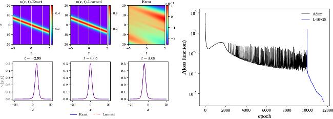
Figure 1. The left-upper three figures give the theoretical, simulative, and pointwise error contours for the one-soliton solver of the Boussinesq equation. Comparisons of the theoretical and the predicted results at three different time diagnosis points are shown in the left-lower three plots. The right plot is the loss function versus the epoch. |
3.2. Two-soliton solution
The two-soliton solutions of the Boussinesq equation are then numerically simulated by the data-driven IPINNs model with physics information. The colliding-soliton and chasing-soliton are the two states of the two-soliton solutions for the Boussinesq equation. The values of parameters k1, k2 and the signs of parameters ω1, ω2 in equation (6 ) can determine the soliton model. The IB conditions with different parameters are described in the following equation [39, 40], which provides the IB training data to the deep neural network model,
$\begin{eqnarray}\left\{\begin{array}{ll}I(x)=u[x,-5]=\frac{2A(0,x)}{C(0,x)}-\frac{2{B}^{2}(0,x)}{{C}^{2}(0,x)},\quad & x\in [-20,20],\\ B(t)=u[\pm 20,t]=\frac{2A(t,\pm 20)}{C(t,\pm 20)}-\frac{2{B}^{2}(t,\pm 20)}{{C}^{2}(t,\pm 20)},\quad & t\in [-5,5],\end{array}\right.\end{eqnarray}$
where the initial loss term about the first-order derivative with respect to time is not listed here as the above one-soliton simulation. The simulation domain is also chosen as t ∈ [−5, 5], x ∈ [−20, 20] to do comparison with the former work. Parameter scans of k1 and k2 are carried out to verify the versatile application of the current model to find data-driven solutions of the colliding-soliton and chasing-soliton states, respectively. A wide range of parameter combination can fulfil the high prediction accuracies with the relative L2-norm errors around 10−4 as the above one-soliton case. For consistency, the neural network parameters are set to be 5 hidden layers and 30 neurons are included in each hidden layer for the two-soliton simulations.3.2.1. colliding-soliton solution
The colliding-soliton solution for the Boussinesq equation is validated first by the numerical simulation with the deep neural network model. Parameter scans ranging from k1 = k2 = 0.7 to k1 = k2 = 1.7 are executed with value interval of 0.2, where the parameters ω1, ω2 have opposite sign. k will represent k1 and k2 in the following for simplicity due to the same value of k1 and k2 in the colliding-soliton case. The two solitons have the same magnitude but the opposite directions in these conditions giving rise to the colliding-soliton phenomena. Different IB conditions are determined by the above different parameter settings in equation (6 ), leading to distinct loss terms in regard to the IB constraints while maintaining the same loss term describing the physical model. Comparisons of the theoretical and simulative results with k = 0.7, k = 1.1, k = 1.3, and k = 1.7 are shown in figures 2–5 in the spatial and temporal domains. The upper three contour plots, denoted by labels a, b, and c in each case, depict the exact, learned, and pointwise error results. The third plot serves to illustrate the difference between the exact and learned results. The exact and learned results agree with each other very well from the plot (a) and plot (b) in the four cases. A specific value comparison can be obtained from the contour plot (c) with all the domain distributions exhibiting very small values compared to the exact results in each parameter setup. The relative L2-norm errors can be derived from the four simulations that are 4.83 × 10⁻⁴, 5.47 × 10⁻⁴, 6.55 × 10⁻⁴, and 5.69 × 10⁻⁴. Three diagnosis positions in t which are marked by the three white lines in the exact (a) and learned (b) contour plots, are chosen to give the specific comparisons in x direction. Once again, the perfect line overlap reveals the good agreement of exact and learned results as shown in the lower three plots labeled by (d), (e), and (f) in the four parameter settings. These results collectively affirm the high prediction accuracies achieved by the current model under different IB conditions.
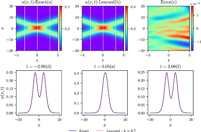
Figure 2. The upper three figures give the exact, learned, and pointwise error contours for k = 0.7 in the colliding-soliton simulations. Comparisons of the theoretical and the predicted results at three different time diagnosis points are shown in the lower three plots. |
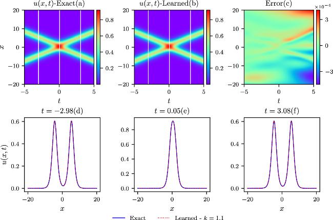
Figure 3. The comparisons of the exact and learned results are depicted similarly to those in the above figure 2, except that k = 1.1 in the colliding-soliton simulations. |
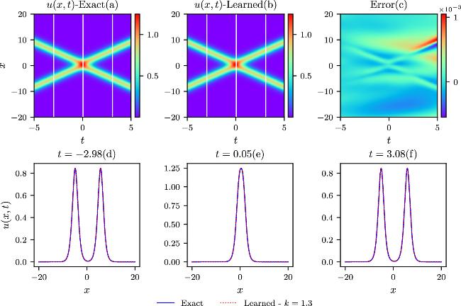
Figure 4. The comparisons of the exact and learned results are depicted similarly to those in the above figure 2, except that k = 1.3 in the colliding-soliton simulations. |
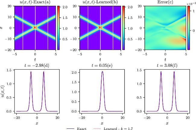
Figure 5. The comparisons of the exact and learned results are depicted similarly to those in the above figure 2, except that k = 1.7 in the colliding-soliton simulations. |
The best relative L2-norm errors and the training time with respect to the k1 and k2 parameters are exhibited in table 2. Here, J1 represents the IPINNs model, and J2 represents the PINNs model, which also applies to the following description. The relative L2-norm error is denoted as L2 error in the Table for simplicity. The best relative L2-norm errors are above two orders smaller than the results in former research [41] with k = 1.1 in the J1 simulation. Furthermore, the parameter range of k1 and k2 is considerably wider, indicating better robustness in data-driven learning. Training time increases as the values of k1 and k2 grow from k = 0.7 to k = 1.7. From the theoretical result of the Boussinesq equation in equation (6 ), it can be known that the two colliding-soliton widths are narrower with larger k1 and k2 values. Contour plots of the learned results in figures 2 and 3 exhibit the same phenomena in the simulation domains in the four parameter settings. Collision areas in spatial and temporal domains are greatly correlated with the width of the solitons as seen from the contour plots. From the traditional mesh-based point of view, the narrow soliton width means the grid resolution in spatial and temporal domains should increase for the simulation. The deep neural network model follows the same rule in the current simulations in solving the colliding-soliton solutions for the Boussinesq equation. To evaluate the performance of the deep learning model, the training times in table 2 are analyzed, incorporating the figure plots. The width of the k = 0.7 soliton in figure 2 is approximately 3.5 times wider than that of the k = 1.7 case in figure 5. Additionally, the training time is about 11.0 times longer for the soliton with k = 1.7 than that for the k = 0.7 case from table 2. However, the increased training time for the k = 1.7 soliton using the finite difference method with traditional mesh grids would exceed two orders of magnitude longer than that for the k = 0.7 case due to the CFL condition. The application of automatic differentiation computation can reduce the increased time for the fourth-order derivative in x direction and second-order derivative in t direction. For the J2 simulations, all the description are similar except that the relative L2-norm errors are much larger due to the ignorance of the initial first-order time derivative term in the loss function. Still, the relative L2-norm errors are about 3 times smaller than the results in former research [41].
Table 2. The training time and relative L2-norm errors are given by scanning the parameters k1, k2 for the colliding-soliton solver of the Boussinesq equation. |
| k1, k2 | 0.7 | 0.9 | 1.1 | 1.3 | 1.5 | 1.7 |
|---|---|---|---|---|---|---|
| L2 error(10−4)-J1 | 4.83 | 4.48 | 5.47 | 6.55 | 6.72 | 5.69 |
| L2 error(10−2)-J2 | 1.47 | 2.87 | 2.60 | 1.95 | 1.60 | 3.90 |
| time-J1 | 6 m 42 s | 13 m 23 s | 15 m 21 s | 23 m 34 s | 42 m15 s | 1 h 6 m |
| time-J2 | 6 m17 s | 12 m 42 s | 16 m 57 s | 25 m 16 s | 41 m 52 s | 1 h 9 m |
In figure 6, the loss function evolutions are given with the k1 and k2 parameters setups from table 2 by the Adam optimizer plus the L-BFGS algorithm with the IPINNs model. The total number of training epochs increases from the k = 0.7 parameter setting to the k = 1.7 case in the current simulations. Since the neural network architecture, the number of collocation points and IB points, and the physics information are the same, the total training time is closely related to the optimizer steps. The number of the Adam optimizer iteration is set as 10 000, so the increasing time comes from the L-BFGS iterations. The learning speed is slower for the narrower width of the colliding-soliton for the L-BFGS algorithm. Each epoch consumes more time due to the second-order derivatives of the loss function with the L-BFGS algorithm compared to the Adam optimizer, with the latter relying only on the first-order derivatives.
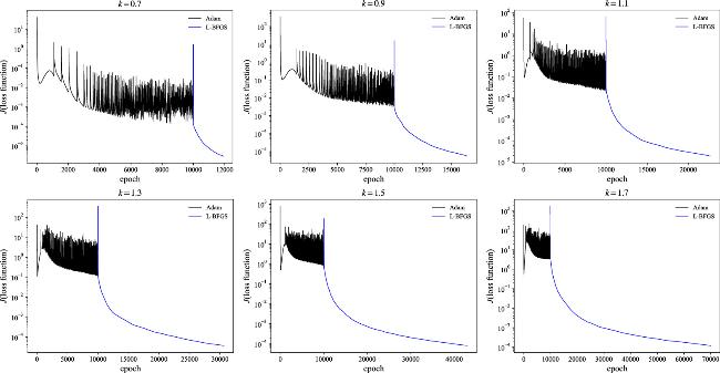
Figure 6. The six plots give the evolution of the loss function in the training process versus epoch by scanning parameter from k = 0.7 to k = 1.7 for the colliding-soliton case. |
The current simulations employ the TANH activation function in the neural networks. In table 3, we provide descriptions and comparisons of the TANH, SIN (sinusoidal), GELU (Gaussian Error Linear Unit), SWISH, and MISH activation functions using the k = 1.1 case. The best relative L2-norm errors achieved are 1.03 × 10⁻², 6.09 ×10⁻⁴, 6.35 × 10⁻⁴, and 7.33 × 10⁻⁴ for the SIN, GELU, SWISH, and MISH methods, respectively. The GELU, SWISH, and MISH activation functions achieve prediction accuracies comparable to that of the TANH function. In contrast, the sinusoidal activation functions demonstrate significantly poorer prediction precision. Additionally, the ReLU (Rectified Linear Unit) and Leaky ReLU activation functions fail to produce valid results or encounter NaN (Not a Number) issues in the current simulations. The training times for the SIN, GELU, SWISH, and MISH activation functions are approximately 2.37, 3.16, 1.86, and 1.77 times slower, respectively, compared to the TANH case. In figure 7, the evolutions of the loss function are shown, with Adam iterations set to 10 000, consistent with the above setup. The GELU, SWISH, and MISH activation functions achieve similar final loss values, as illustrated in the upper right figure of figure 6. However, despite having comparable training epochs to the TANH case, the SWISH and MISH activation functions exhibit slower per-epoch training times, resulting in longer total training durations. These comparisons confirm that the TANH activation function is efficient for the current simulations.
Table 3. The training time and relative L2-norm errors are evaluated for different activation functions in the k = 1.1 case of the colliding-soliton. |
| k = 1.1 | TANH | SIN | GELU | SWISH | MISH |
|---|---|---|---|---|---|
| L2 error(10−4)-J1 | 5.47 | 103 | 6.09 | 6.35 | 7.33 |
| time-J1 | 15 m 21 s | 36 m 32 s | 48 m 25 s | 28 m 34 s | 27 m 10 s |
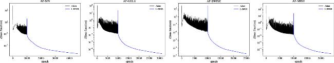
Figure 7. The three plots illustrate the evolution of the loss function using sinusoidal, SWISH, and MISH activation functions for the k2 = 1.1 colliding-soliton case. |
3.2.2. Chasing-soliton solution
The chasing-soliton phenomena arise when two solitons move in the same direction but have different magnitudes. Parameter scans from k2 = 0.7 to k2 = 1.7 with a value interval of 0.2 are simulated at k1 = 1.5, and the parameters ω1 and ω2 have the same sign. Different IB conditions are determined by the above different parameter settings in equation (6 ), allowing for the regularization of the same physical model. The total loss terms, governed by different IB constraints, are optimized using the Adam optimizer in conjunction with the L-BFGS algorithm in the IPINNs model. Exact and learned results are compared for k2 = 0.7, k2 = 1.1, k2 = 1.5, and k2 = 1.7 at k1 = 1.5 in figures 8–11 in the spatial and temporal domains. The three upper contour plots, designated as (a), (b), and (c), share a resemblance to the earlier colliding-soliton case in their description. Pointwise error values(c), observed from the contour plots, are very small compared to the exact values. Relative L2-norm errors, derived from the four pointwise error distribution plots (c), are 4.82 × 10⁻⁴, 5.22 × 10⁻⁴, 2.47 × 10⁻⁴, and 5.73 × 10⁻⁴, indicating high prediction accuracies under varying IB conditions. In the lower three plots labeled by d, e, and f of the four parameter settings (marked by three white lines in the exact and learned contour plots in figures 8–11), the blue solid lines and red dotted lines affirm the good agreement between exact and learned results.
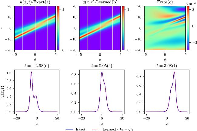
Figure 8. The upper three figures give the exact, learned, and pointwise error contours for k2 = 0.9 in the chasing-soliton simulations. Comparisons of the theoretical and the predicted results at three different time diagnosis points are shown in the lower three plots. |
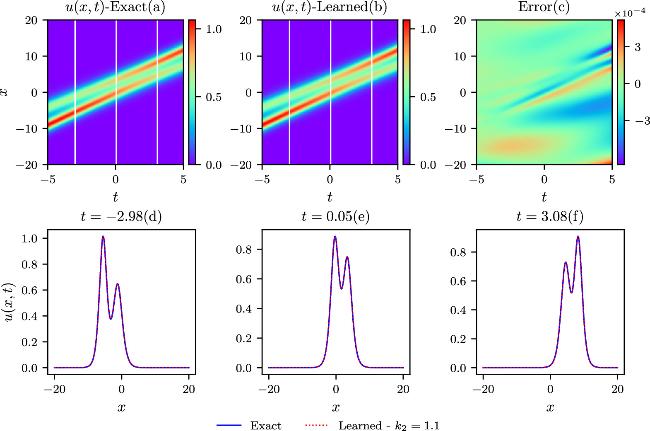
Figure 9. The comparisons of the exact and learned results are depicted similarly to those in the above figure 8, except that k = 1.1 in the chasing-soliton simulations. |
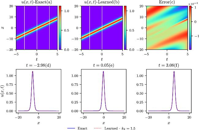
Figure 10. The comparisons of the exact and learned results are depicted similarly to those in the above figure 8, except that k = 1.5 in the chasing-soliton simulations. |
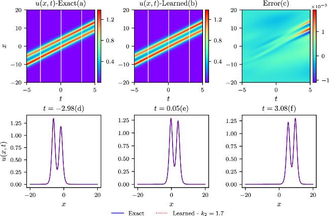
Figure 11. The comparisons of the exact and learned results are depicted similarly to those in the above figure 8, except that k = 1.7 in the chasing-soliton simulations. |
The relative L2-norm errors and the training time with respect to the k2 parameters at k1 = 1.5 are shown in table 4. Notably, for the parameter setup of k2 = 0.9 at k1 = 1.5, the best relative L2-norm errors surpass those reported in previous research [41] by more than two orders of magnitude in J1 simulation. In addition, the comprehensive parameter scans across a wide range of k2 values validate the model’s robustness in the context of chasing-soliton simulations. The training time exhibits a slight increase from k2 = 0.7 to k2 = 1.3 due to that the other parameter k1 is fixed at 1.5 determining one soliton width in the physical process. When the condition k2 = k1 = 1.5 meets, two solitons merge into one soliton, leading to a simple structure in the spatial and temporal domains with the training time significantly decreasing. It should be noted that when the condition k2 ≪ k1 is satisfied, the two solitons would undergo a similar transformation into one soliton. When k2 is around 0.9 at k1 = 1.5, a notable phase shift phenomenon occurs, marked by a separation-fusion-separation process. The amplitude of the dominant soliton remains almost unchanged before and after the interaction but decreases during the fusion process in the simulation. For the simulations with k2 = 1.1, 1.3, 1.7 at k1 = 1.5, the interactions between the two chasing solitons remain strong, but the fusion phenomena are less prominent. For the J2 simulations, the relative L2-norm errors are significantly larger compared to the J1 cases, similar to the aforementioned colliding-soliton simulations, except for the case when k2 = k1 = 1.5. The relative L2-norm error is approximately 50% smaller than the result reported in the k2 = 0.9 case, which is solely provided in the previous research [41].
Table 4. The training time and relative L2-norm errors are given by scanning the parameters k2 at k1 = 1.5 for the chasing-soliton solver of the Boussinesq equation. |
| k2 | 0.7 | 0.9 | 1.1 | 1.3 | 1.5 | 1.7 |
|---|---|---|---|---|---|---|
| L2 error(10−4)-J1 | 4.50 | 4.82 | 5.22 | 4.63 | 2.47 | 5.73 |
| L2 error(10−2)-J2 | 5.90 | 4.64 | 5.80 | 4.14 | 0.054 | 4.51 |
| time-J1 | 15 m 44 s | 17 m 4 s | 23 m 41 s | 23 m 55 s | 8 m 32 s | 38 m 40 s |
| time-J2 | 16 m 23 s | 17 m 32 s | 21 m 52 s | 26 m 23 s | 8 m 15 s | 47 m 52 s |
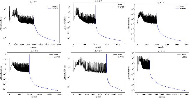
The evolution of the loss function is depicted in figure 12 concerning the k2 parameters at k1 = 1.5 with the IPINNs model. The optimization is performed using the Adam optimizer in conjunction with the L-BFGS algorithm. The neural network architecture, the number of collocation points and IB points, and the physics information are the same as in the above colliding-soliton cases. The number of the Adam optimizer iteration is set as 10 000, and the observed increase in training time is primarily attributed to the L-BFGS iterations. The total number of training epochs via the L-BFGS algorithm correlates significantly with the training time outlined in table 4. The longer training time for the k2 = 1.7 case at k1 = 1.5 can be attributed to the interaction of two solitons with narrower widths, resembling the colliding-soliton scenario discussed earlier. The L-BFGS algorithm requires more training epochs under such conditions. Conversely, the number of epochs decreases considerably for the k2 = 1.5 case at k1 = 1.5, where one soliton is formed by the fusion of two solitons.
Figure 12. The six plots give the evolution of the loss function in the training process versus epoch by scanning parameter from k2 = 0.7 to k2 = 1.7 for the chasing-soliton case. |
4. Conclusions and discussion
The IPINNs model has been employed to study one-soliton and two-soliton wave solutions for the fourth-order Boussinesq equation, providing insights into the dynamic behavior and interaction between solitons. The loss function, accounting for the Boussinesq equation’s second-order time dependence, includes a new initial first-order time derivative term, which is crucial for achieving high prediction accuracy. Adaptive activation function mechanism and loss-balanced coefficients are utilized to accelerate and enhance the PINNs model, as highlighted in previous research [10, 12, 42, 45]. The IPINNs model achieves high prediction accuracy, with relative L2-norm errors around 10−4. This represents a significant improvement, with prediction precision increased by two orders of magnitude compared to previous results [41]. Comparisons among the TANH, SIN, GELU, SWISH, and MISH activation functions in the neural network are conducted using the colliding-soliton k = 1.1 case, confirming that the selection of TANH activation function is efficient for the current simulations. To validate the versatility and robustness of the IPINNs model, parameter scans are conducted for the two-soliton wave solvers of the Boussinesq equation. The training time is found to be closely related to the width of the two-soliton solutions when using the L-BFGS algorithm during colliding-soliton simulations. For instance, the width of the soliton with k = 1.7 is approximately 3.5 times narrower than that of the k = 0.7 case, with a corresponding training time that is about 11 times longer. However, the increased training time is not as pronounced as in traditional mesh-based algorithms, thanks to the use of automatic differentiation for the fourth-order Boussinesq equation. In the chasing-soliton scenario, when the condition k2 = k1 = 1.5 is met, the two solitons merge into one, resulting in a significant reduction in training time. The current model requires more initial data, which presents a challenge in obtaining the additional information.
The widespread applications of the PINNs software in solving NPDEs still require further understanding and optimization, as its prediction abilities are unstable in certain scenarios. To enhance the generalizability of deep neural network models, attention should be directed towards numerous NPDEs in physical fields that have yet to be solved using PINNs software. For instance, the modified Korteweg-de Vries–sine-Gordon equation, which describes few-cycle-pulse optical solitons and features rich structures such as soliton molecules, breather molecules, and breather-soliton molecules, presents a challenging problem for the PINNs model. Laser physics phenomena associated with the Boussinesq model will be studied in the future using the current model to assess its capability [51–53]. The soliton and lump solutions of the (2 + 1)-dimensional (3D) generalized variable-coefficient Hirota-Satsuma-Ito equation are worthy of study with the current model to verify its robustness and efficiency [54]. The computational efficiency of the current model when applied to 3D PDEs is a potential challenge and requires further study. For 3D PDEs with solutions exhibiting locally steep gradients or high-frequency components, adaptive sampling methods [16] and self-adaptive weight algorithms with scalable multi-GPU support [55] emerge as promising candidate approaches. The SAEE-PINN model using sparse data also provides valuable insights for our future research [28]. For PDEs with high-order or irregular domains, PINNs with a mesh-free method offer advantages over traditional methods that rely on mesh grid techniques [16, 56]. Future research will compare the current multilayer perceptron to the Kolmogorov–Arnold representation, which is also receiving attention in PINNs research. Combining domain decomposition techniques [15, 57, 58] with the current IPINNs model offers a promising approach for conducting large-domain simulations with higher prediction accuracy. Further advancements in heterogeneous parallel computing would significantly accelerate training through distributed data-parallel methods, which adjust the mini-batch sizes across workers. Incorporating more accelerated computing platforms in software development will also enhance the versatility and efficiency of software execution. Upgrading from TensorFlow 1 to TensorFlow 2 will be completed in our further work, improving support for distributed computing, automatic mixed precision, and other optimizations.
Declaration of competing interest
The authors declare that they have no conflict of interest.
Ethical standards
This research does not involve human participants and/or animals.