


1. Introduction
In the absence of external stimulation, neurons maintain a voltage difference across their cell membranes, known as the resting potential. The resting membrane potential (Em) and the reversal potential of gamma-aminobutyric acid (GABA)-induced anionic currents (EGABA) are key factors that control neuronal excitability [1–3]. When neurons are stimulated, their membrane potential reverses, causing them to enter an excited state. Excited neurons can exhibit four discharge modes: periodic firing, chaotic bursting, and spiking [4–7]. Nonlinear circuits exhibit complex dynamical behaviors, and by tuning parameters, these circuits can replicate discharge patterns similar to those observed in neurons [8–11]. The nonlinear effects of biological membranes can be modeled using appropriate nonlinear models [12].
Functional neurons gather various types of information from the environment, requiring corresponding functional devices for equivalent modeling. For example, photoreceptive neurons detect external light signals. Lewicki et al [13] discussed how photoreceptors process visual information through structural and functional segregation: the outer segment absorbs light and initiates the visual signal transduction process, while the synaptic terminal transmits the signal to the next neuron in the visual pathway. Liu et al [14] constructed photoreceptive neuron models by integrating photodiodes into nonlinear circuits. Similarly, Zhou et al [15] suggested using piezoelectric ceramics to build auditory neurons, while Rubel et al [16] reviewed the development and information transmission of cochlear neurons. Josephson junctions [17, 18] can simulate the effects of external magnetic fields on neurons, and thermistors [19, 20] can be used to construct thermosensitive neuron circuits. Nenova et al [21] proposed a linearized circuit connected with a thermistor. Yang et al [22] calculated adaptive coupling with memristor channels.
In neuron circuits, sensing devices must convert signals from other forms into electrical signals to modulate the system’s dynamical behavior [23–26]. As dynamical systems, neurons follow Helmholtz’s theorem [27], and neuron models based on nonlinear circuits also satisfy this theorem [28]. Some neurons self-regulate their activities by releasing inhibitory or excitatory neurotransmitters, which helps control their firing frequency and pattern [29–33]. This feedback mechanism can be implemented in nonlinear circuits through negative feedback regulation [34, 35]. Additionally, Sprott et al [36] showed that parameter tuning can change the output potential state of the circuit. Based on the current research, this study constructs a neuron model, investigates its dynamical behavior, and achieves targeted regulation of time-varying parameters using energy criteria and exponential gain methods.
2. Model and Scheme
In neuron models, the inner and outer membrane of cells can be described by two capacitors, ion channels are equivalent to inductors [6, 37]. Chua’s circuit has two capacitors and complex dynamic behavior [38–42]. We based this on the Chua’s circuit, reducing neuronal ion (Na+, K+, Cl− etc) channels to an inductor coil, The ion interaction between double membrane is realized by a resistor,the nonlinear resistance (NR) represents the nonlinear effect caused by the change of neuronal membrane fluidity. Josephson junction has superconducting quantum effects and magnetic sensitivity. Its quantum property is not considered here, and it is used as a magnetic field sensitive element to sense magnetic fields. Phototube is a photosensitive device [43]. In summary, the neuron circuit model shown in figure 1 can be constructed.
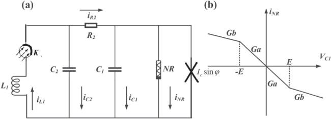
Figure 1. (a) Double membrane, magnetic sensitive, light sensitive neuron model constructed by Chua’s circuit. (b) I-V characteristic curve of the Chua’s diode, it’s a nonlinear resistance (NR). |
In figure 1, K is a phototube, L1 equivalent ion channel, and C1 and C2 equivalent double-layer membranes of neurons. Ic sin φ is the output current of the Josephson junction, it is equivalent to the neuron’s perception for surrounding magnetic field. Ic represents the maximum junction current of the Josephson junction here, φ represents the magnetic field phase difference between two ends of the junction. R2 is used for double-layer membrane communication. The current and voltage relationship of the Josephson junction can be expressed as equation (1 ).
$\begin{eqnarray}\displaystyle \frac{\hslash }{2e}\displaystyle \frac{{\rm{d}}\varphi }{{\rm{d}}t}={V}_{C1},\,I={I}_{C}\,\sin \left(\varphi \right).\end{eqnarray}$
From equation (1 ), Josephson is a current source and a magnetic field sensitive element here [44–47], The circuit’s current and voltage analysis can be derived from equation (2 ).
$\begin{eqnarray}\left\{\begin{array}{lll}{C}_{1}\displaystyle \frac{{\rm{d}}{V}_{C1}}{{\rm{d}}t} & = & \displaystyle \frac{{V}_{C2}-{V}_{C1}}{{R}_{2}}-{i}_{NR}-{I}_{C}\,\sin \left(\varphi \right),\\ {C}_{2}\displaystyle \frac{{\rm{d}}{V}_{C2}}{{\rm{d}}t} & = & {i}_{L1}-\displaystyle \frac{{V}_{C2}-{V}_{C1}}{{R}_{2}},\\ {L}_{1}\displaystyle \frac{{\rm{d}}{i}_{L1}}{{\rm{d}}t} & = & -{V}_{C2}-{V}_{K},\\ \displaystyle \frac{{\rm{d}}\varphi }{{\rm{d}}t} & = & \displaystyle \frac{2e}{\hslash }{V}_{C1}.\end{array}\right.\end{eqnarray}$
In equation (2 ), VC1 and VC2 represent the voltage at both ends of C1 and C2, respectively. VK represents K’s voltage, iL1 flows through L1 and K, In figure 1, NR represents the Chua’s diode [48]. iNR represents the current flowing through the Chua’s diode, the current and voltage relationship of the Chua’s diode can be expressed as [49],
$\begin{eqnarray}{i}_{NR}={G}_{a}{V}_{C1}+0.5\left({G}_{b}-{G}_{a}\right)\left(\left|{V}_{C1}+E\right|-\left|{V}_{C1}-E\right|\right).\end{eqnarray}$
For the convenience of research, the physical quantity in equations (2 ) and (3 ) is dimensionless and transformed as follows,
$\begin{eqnarray}\left\{\begin{array}{lll}x & = & \displaystyle \frac{{V}_{C1}}{E},\,y=\displaystyle \frac{{V}_{C2}}{E},\,z=\displaystyle \frac{{i}_{L1}{R}_{2}}{E},\\ \tau & = & \displaystyle \frac{t}{{R}_{2}{C}_{2}};\,\alpha =\displaystyle \frac{{C}_{2}}{{C}_{1}},\,\beta =\displaystyle \frac{{C}_{2}{R}_{2}^{2}}{{L}_{1}},\\ {u}_{K} & = & \displaystyle \frac{{V}_{K}}{E},\,{m}_{0}={R}_{2}{G}_{b},\,{m}_{1}={R}_{2}{G}_{a},\\ {I}_{c} & = & \displaystyle \frac{{I}_{C}{R}_{2}}{E},\,\phi =\varphi ,\,d=\displaystyle \frac{2eE{R}_{2}{C}_{2}}{\hslash }.\end{array}\right.\end{eqnarray}$
Note that $\varphi $ is a dimensionless quantity, which is replaced by $\phi $, and both represent the phase difference of the superconducting wave functions at the two ends of the junction. [50]. Combining equations (2 ) and (4 ) can obtain equation (5 ).
$\begin{eqnarray}\left\{\begin{array}{c}\dot{x}=\alpha (y-x)-\alpha f(x)-\alpha {I}_{c}\,\sin \,\phi ,\\ \dot{y}=x-y+z,\\ \dot{z}=-\beta (y+{u}_{K}),\\ \dot{\phi }=dx.\end{array}\right.\end{eqnarray}$
In equation (5 ), the current across NR defined in equation (3 ) can be updated in a dimensionless form as follows,
$\begin{eqnarray}f(x)={m}_{1}x+0.5\left({m}_{0}-{m}_{1}\right)\left(| x+1| -| x-1| \right).\end{eqnarray}$
The photocell exists as a voltage source. The Josephson junction as a current source. They can sense the photo and magnetic fields in the environment of neurons respectively, and then jointly realize the regulation of the neuronal firing mode.
The system satisfies Helmholtz’s theorem [51–54]. In Helmholtz’s theorem, Fc(X) and Fd(X) are the gradient field and vortex field in vector field F(X). The relationship among Fc(X) and Fd(X) and equation (5 ) is as follows,
$\begin{eqnarray}\left\{\begin{array}{l}{\rm{\nabla }}{H}^{{\rm{T}}}{F}_{c}\left(X\right)\,=\,0,\,\dot{H}=\displaystyle \frac{{\rm{d}}H}{{\rm{d}}\tau }={\rm{\nabla }}{H}^{{\rm{T}}}{F}_{{\rm{d}}}\left(X\right),\\ \displaystyle \frac{{\rm{d}}X}{{\rm{d}}\tau }\,=\,F\left(X\right)={F}_{c}\left(X\right)+{F}_{{\rm{d}}}\left(X\right),\,X\subset {R}^{N}.\end{array}\right.\end{eqnarray}$
According to equation (7 ), (5 ) can be decomposed as follows,
$\begin{eqnarray*}\begin{array}{lll}\left(\begin{array}{c}\dot{x}\\ \dot{y}\\ \dot{z}\\ \dot{\phi }\end{array}\right) & = & {F}_{c}+{F}_{{\rm{d}}}=\left(\begin{array}{c}\alpha (y-x)-\alpha f(x)-\alpha {I}_{c}\,\sin \,\phi \\ x-y+z\\ -\beta (y+{u}_{K})\\ dx\end{array}\right)\\ & = & \left(\begin{array}{c}\alpha y+\alpha \displaystyle \frac{{I}_{c}}{{\rm{d}}}\,\sin \,\phi \\ x+z\\ -\beta y\\ x\end{array}\right)\\ & & +\left(\begin{array}{c}-\alpha f(x)-\alpha x-\displaystyle \frac{\alpha ({I}_{c}+d{I}_{c})\sin \,\phi }{d}\\ -y\\ -\beta {u}_{K}\\ (d-1)x\end{array}\right)\end{array}\end{eqnarray*}$
$\begin{eqnarray}\begin{array}{lll} & = & \left[\begin{array}{cccc}0 & \alpha & 0 & \alpha \\ -\alpha & 0 & \beta & 0\\ 0 & -\beta & 0 & 0\\ -\alpha & 0 & 0 & 0\end{array}\right]\left[\begin{array}{c}-\displaystyle \frac{x}{\alpha }\\ y\\ \displaystyle \frac{z}{\beta }\\ \displaystyle \frac{{I}_{c}}{d}\,\sin \,\phi \end{array}\right]\\ & & +\left[\begin{array}{cccc}{F}_{{\rm{d}}11} & 0 & 0 & 0\\ 0 & -1 & 0 & 0\\ 0 & 0 & \displaystyle \frac{-{\beta }^{2}{u}_{K}}{z} & 0\\ 0 & 0 & 0 & \displaystyle \frac{(d-1)dx}{{I}_{c}\,\sin \,\phi }\end{array}\right]\left[\begin{array}{c}-\displaystyle \frac{x}{\alpha }\\ y\\ \displaystyle \frac{z}{\beta }\\ \displaystyle \frac{{I}_{c}}{d}\,\sin \,\phi \end{array}\right],\\ {F}_{{\rm{d}}11} & = & \displaystyle \frac{{\alpha }^{2}f(x)}{x}+{\alpha }^{2}+\displaystyle \frac{{\alpha }^{2}({I}_{c}+d{I}_{c})\sin \,\phi }{dx}.\end{array}\end{eqnarray}$
The field energy of the neuron be saved in the C1, C2, L1, Josephson junction. Over time, energy is exchanged within these devices. So, the energy of the neuron in figure 1 can be represented as equation (9 ).
$\begin{eqnarray}\begin{array}{lll}W & = & {W}_{C1}+{W}_{C2}+{W}_{L1}+{W}_{J}\\ & = & -\displaystyle \frac{1}{2}{C}_{1}{{V}_{C1}}^{2}+\displaystyle \frac{1}{2}{C}_{2}{{V}_{C2}}^{2}+\displaystyle \frac{1}{2}{L}_{1}{{i}_{L1}}^{2}+\displaystyle \int {V}_{C1}{I}_{C}\,\sin \,\varphi {\rm{d}}t\\ & = & -\displaystyle \frac{1}{2}{C}_{1}{{V}_{C1}}^{2}+\displaystyle \frac{1}{2}{C}_{2}{{V}_{C2}}^{2}+\displaystyle \frac{1}{2}{L}_{1}{{i}_{L1}}^{2}-\displaystyle \frac{{I}_{C}\hslash }{2e}\,\cos \,\varphi .\end{array}\end{eqnarray}$
In equation (9 ), WC1, WC2, WL1, WJ denote the field energy being stored as C1, C2, L1 and the Josephson junction presently. The dimensionless variation of equation (9 ) gives the Hamilton energy of the system as equation (10 ).
$\begin{eqnarray}\begin{array}{lll}H & = & \displaystyle \frac{W}{{C}_{2}{E}^{2}}=\displaystyle \frac{{W}_{C1}}{{C}_{2}{E}^{2}}+\displaystyle \frac{{W}_{C2}}{{C}_{2}{E}^{2}}+\displaystyle \frac{{W}_{L1}}{{C}_{2}{E}^{2}}+\displaystyle \frac{{W}_{J}}{{C}_{2}{E}^{2}}\\ & = & {H}_{C1}+{H}_{C2}+{H}_{L1}+{H}_{J}\\ & = & -\displaystyle \frac{1}{2\alpha }{x}^{2}+\displaystyle \frac{1}{2}{y}^{2}+\displaystyle \frac{1}{2\beta }{z}^{2}-\displaystyle \frac{{I}_{c}}{d}\,\cos \,\phi .\end{array}\end{eqnarray}$
In equation (10 ), HC1, HC2, HL1, HJ denote the dimensionless field energy of C1, C2, L1 and the Josephson junction [55–58]. The proportions of the energy of C1, C2, L1 and the Josephson junction to the Hamilton energy is expressed as
$\begin{eqnarray}\left\{\begin{array}{lll}{p}_{1} & = & \left|\displaystyle \frac{\lt {H}_{C1}\gt }{{H}_{{\rm{a}}{\rm{l}}{\rm{l}}}}\right|,\,{p}_{2}=\left|\displaystyle \frac{\lt {H}_{C2}\gt }{{H}_{{\rm{a}}{\rm{l}}{\rm{l}}}}\right|,\\ {p}_{3} & = & \left|\displaystyle \frac{\lt {H}_{L1}\gt }{{H}_{{\rm{a}}{\rm{l}}{\rm{l}}}}\right|,\,{p}_{4}=\left|\displaystyle \frac{\lt {H}_{J}\gt }{{H}_{{\rm{a}}{\rm{l}}{\rm{l}}}}\right|,\\ {H}_{{\rm{a}}{\rm{l}}{\rm{l}}} & = & \left|\lt {H}_{C1}\gt \right|+\left|\lt {H}_{C2}\gt \right|+\left|\lt {H}_{L1}\gt \right|+\left|\lt {H}_{J}\gt \right|.\end{array}\right.\end{eqnarray}$
Equation (5 ) and (10 ) can be substituted into equation (7 ) to obtain equation (12 ).
$\begin{eqnarray}\left\{\begin{array}{l}{\rm{\nabla }}{H}^{{\rm{T}}}{F}_{c}(X)\,=\,\left(\alpha y+\alpha \displaystyle \frac{{I}_{c}}{d}\,\sin \,\phi \right)\left(-\displaystyle \frac{x}{\alpha }\right)+\left(x+z\right)y\\ -\beta y\displaystyle \frac{z}{\beta }+\displaystyle \frac{{I}_{c}}{d}x\,\sin \,\phi =0,\\ \dot{H}\,=\,\displaystyle \frac{{\rm{d}}H}{{\rm{d}}\tau }=\displaystyle \frac{{\rm{d}}H}{{\rm{d}}X}\displaystyle \frac{{\rm{d}}X}{{\rm{d}}\tau }={\rm{\nabla }}{H}^{{\rm{T}}}\left[{F}_{c}(X)\right.\\ \left.+{F}_{d}(X)\right]={\rm{\nabla }}{H}^{{\rm{T}}}{F}_{d}\left(X\right).\end{array}\right.\end{eqnarray}$
It is proven that equation (5 ) and (10 ) satisfy Helmholtz’s theorem, so the Hamiltonian energy can be used as the system energy for calculation. In fact, neurons can dynamically adjust their behavior based on variations in energy and state [6, 59]. Additionally, synapses in neurons possess self-regulating mechanisms [60]. This work utilizes the stored field energy in various components, combined with an exponential gain method, to achieve control over system parameters, expressed as follows,
$\begin{eqnarray}\left\{\begin{array}{lll}\displaystyle \frac{{\rm{d}}\alpha \left(\tau \right)}{{\rm{d}}\tau } & = & {\sigma }_{1}\alpha \left(\tau \right)K\left({H}_{C1}-{\varepsilon }_{1}\right),\,K\left(p\right)=1,\\ & & p\geqslant 0,\,K\left(p\right)=0,\,p\lt 0,\\ \displaystyle \frac{{\rm{d}}\beta \left(\tau \right)}{{\rm{d}}\tau } & = & {\sigma }_{2}\beta \left(\tau \right)K\left({H}_{L1}-\varepsilon \right),\,K\left(p\right)=1,\\ & & p\geqslant 0,\,K\left(p\right)=0,\,p\lt 0.\end{array}\right.\end{eqnarray}$
In equation (13 ), ${\sigma }_{1}$ and ${\sigma }_{2}$ represent the gain coefficients for the time-varying parameters $\alpha (\tau )$ and $\beta (\tau )$, respectively. HC1 and HL1 denote the electric field energy stored in C1 and the magnetic field energy stored in L1, respectively. Given that ‘lower energy equals higher stability’, K(p) represents the Heaviside function, and the parameter $\varepsilon $ serves as a threshold to determine whether the energy of the components in the system fall below $\varepsilon $. From equation (13 ), by assigning a small initial value ${\alpha }_{0}$ to $\alpha (\tau )$ with a gain ${\sigma }_{1}$ > 0, when ${H}_{C1}\gt {\varepsilon }_{1}$, the time-varying parameter $\alpha (\tau )$ will continuously increase over time until ${H}_{C1}\leqslant {\varepsilon }_{1}$, at which point $\alpha (\tau )$ stabilizes. Similarly, by assigning a larger initial value ${\beta }_{0}$ to $\beta (\tau )$ with ${\sigma }_{2}$ < 0, when ${H}_{L1}\gt {\varepsilon }_{2}$, $\beta (\tau )$ will continuously decrease over time until ${H}_{L1}\leqslant {\varepsilon }_{2}$, at which point $\beta (\tau )$ stabilizes.
3. Calculation results and analysis
In this section, the solutions for equation (5 ) are calculated by using the fourth-order Runge–Kutta algorithm iteratively, and the time step is fixed at h = 0.01.
First, the voltage variation caused by the fixed external magnetic field’s influence on the Josephson junction, denoted as ${I}_{c}\,\sin \,\phi ,\left({I}_{c}=8,\,{\phi }_{0}=2\right)$. which means we fixed the effect of the external magnetic field on the neuron. We adjust external illumination, induces the photovoltage given by uK = Acos(ωτ). The bifurcation and the Lyapunov exponent (LE) diagrams in the x-direction for varying voltage amplitudes A and angular frequencies ω are illustrated in figure 2.
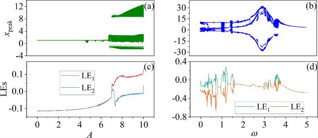
Figure 2. Bifurcation and LEs’diagrams of the uK’s A and ω in the neuron model. The parameters corresponding to the diagrams: (a), (c) ω = 0.01; (b), (d) A = 8.8. Other parameters: $\alpha $ = 10, $\beta $ = 9, Ic = 8, m0 = −1, m1 = 0.9, d = 1. The initial values: (0.1, 0.1, 0.1, 2). |
In figure 2, the fixed external magnetic field, varying the external illumination, the phototube can generate different A and ω, driving the system into distinct oscillation modes. In figures 2(a) and (c), with a fixed ω = 0.01 and gradually increasing the amplitude A at [0, 10], the system transitions from a periodic state to a chaotic state. In figures 2(b) and (d), with a fixed A = 8.8 and gradually increasing the angular frequency ω from 0 to 5, the system exhibits transitions between periodic and chaotic states.
A clearer view of the influence of A's change on the membrane potential, the membrane potential series of the neuron at different A has been calculated, as shown in figure 3.
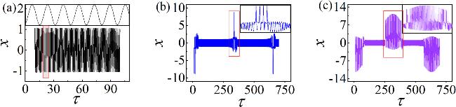
Figure 3. Time sequences of membrane potentials under varying A (the small image is a partial enlargement of the area with red borders). Corresponding A: (a) A = 5; (b) A = 7; (c) A = 9. Other parameters: $\alpha $ = 10, $\beta $ = 9, Ic = 8, m0 = −1, m1 = 0.9, ω = 0.01, d = 1. The initial values: (0.1, 0.1, 0.1, 2). |
From figure 3, it is evident as parameter A gradually increases, the membrane potentials evolve from the periodic state shown in figure 3(a) to the bursting discharge state depicted in figures 3(b) and (c). From a physical perspective, increasing A regulates the neuron’s absorption of energy from the external light field. As A continues to rise, the internal energy storage Components of the system are also adjusted. The ratios of the field energy in each physical component to the Hamiltonian energy at different A are calculated in figure 4.
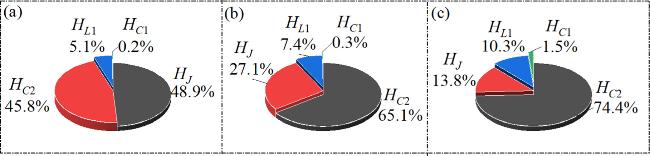
Figure 4. The proportion of field energy in each component to the Hamiltonian energy under different light illumination conditions, (a) A = 5, (b) A = 7, (c) A = 9; Other parameters: $\alpha $ = 10, $\beta $ = 9, Ic = 8, m0 = −1, m1 = 0.9, ω = 0.01, d = 1. The initial values are set to: (0.1, 0.1, 0.1, 2). |
In figure 4(a), it is evident when A = 5, the magnetic field energy stored in the Josephson junction is at its highest, as shown in figure 4(a). At this point, the system exhibits periodic oscillations, as indicated in figure 3(a). When A = 7, the magnetic field energy in the Josephson junction decreases while the electric field energy stored in C2 increases. At this stage, the proportion of electric field energy in C2 to the Hamiltonian energy of the system is maximum, as illustrated in figure 4(b). The neuron then exhibits a clustered discharge state, as depicted in figure 3(b). Furthermore, as the amplitude A rises to A = 9, the energy proportion of C2 reaches 74.4%, as shown in figure 4(c). Additionally, varying ω also drives the system into different states. Figure 5 presents the membrane potentials’time series at varying ω.
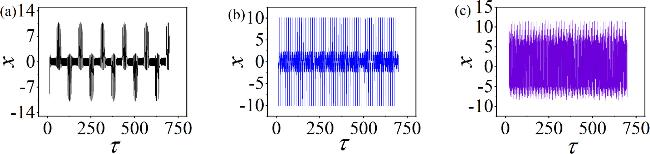
Figure 5. Time sequences of membrane potentials under different ω, with: (a) ω = 0.05; (b) ω = 0.5; (c) ω = 3.5. Other parameters: $\alpha $ = 10, $\beta $ = 9, Ic = 8, m0 = −1, m1 = 0.9, A = 8.8, d = 1. The initial values are set to: (0.1, 0.1, 0.1, 2). |
From figure 5, we find that by adjusting the light field in the environment, the neuron exhibits a clustered discharge when ω = 0.05, as shown in figure 5(a). When ω = 0.5, the neuron demonstrates a spike discharge in figure 5(b), further increasing ω to 3.5 resulting in chaotic discharge, as illustrated in figure 5(c). Combining figures 3 and 5, it is evident that the system can exhibit chaotic, periodic, spiking and bursting. Therefore, the discharge patterns of the neuron can be effectively simulated by this circuit. Similarly, figure 6 show the proportions of field energy in the various components under different oscillation modes resulting from changes in ω.
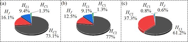
Figure 6. Proportions of energy in various components by different ω. with(a) ω = 0.05; (b) ω = 0.5; (c) ω = 3.5. Other parameters: $\alpha $ = 10, $\beta $ = 9, Ic = 8, m0 = −1, m1 = 0.9, A = 8.8, d = 1. The initial values: (0.1, 0.1, 0.1, 2). |
When the neuron in the clustered discharge in figure 5(a) have ${H}_{C2}\gt {H}_{J}\gt {H}_{L1}\gt {H}_{C1}$ like figure 6(a). When the neuron exhibits a spike discharge in figure 5(b), have ${H}_{C2}\gt {H}_{J}\gt {H}_{L1}\gt {H}_{C1}$ in figure 6(b). Figures 5(a) and (b) have the same orders. Increasing the angular frequency further leads the system into a chaotic state, as ${H}_{L1}\gt {H}_{C2}\gt {H}_{C1}\gt {H}_{J}$ in figure 6(c).
From equation (1 ), We can infer that change in the surrounding magnetic field of the Josephson junction will affect the Josephson current. Therefore, by adjusting the parameters related to the Josephson current maximum Ic and the initial value of the variable φ0, the oscillation state of the membrane potentials can be adjusted. The bifurcation diagram of the membrane potentials concerning the parameters Ic and the initial value of φ0 are presented in figure 7.
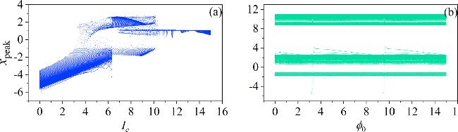
Figure 7. Fixed external illumination, the bifurcation of Josephson current parameter Ic and the initial value of ${\phi }_{0}$. The parameters corresponding to: (a) ${\phi }_{0}$ = 2; (b) Ic = 8. Other parameters: a = 10, b = 9, m0 = −1, m1 = 0.9, $\omega $ = 0.01, A = 8.8, d = 1. The initial values (0.1, 0.1, 0.1). |
In figure 7, increasing Ic facilitates the transition of the system’s oscillation state. However, altering φ0 cannot lead to a state transition. In more detail, we set the Josephson junction current parameters to Ic = 6 and Ic = 11. The resulting membrane potentials’time series are presented in figure 8.
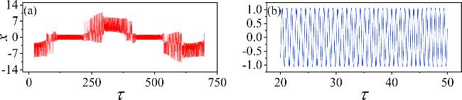
Figure 8. Time series of membrane potential for different Josephson junction current parameters Ic. (a) Ic = 6; (b) Ic = 11. Other parameters: α = 10, β = 9, m0 = −1, m1 = 0.9, $\omega $ = 0.01, A = 8.8, d = 1. The initial values (0.1, 0.1, 0.1, 2). |
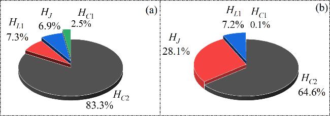
Figure 9. The energy percentage of the individual components under different Ic. (a) Ic = 6; (b) Ic = 11. Other parameters: α = 10, β = 9, m0 = −1, m1 = 0.9, $\omega $ = 0.01, A = 8.8, d = 1. The initial values: (0.1, 0.1, 0.1, 2). |
In equation (10 ), ${H}_{C1}=0.5\alpha {x}^{2},{H}_{L1}=0.5\beta {z}^{2}$, $\alpha ={C}_{2}/{C}_{1},\beta ={C}_{2}{R}_{2}^{2}/{L}_{1}$, The distribution of energy is related to $\alpha ,\beta $. In addition, the membrane potential is equivalent to C1 and C2, and all the channel currents are equivalent to L1. Initially, we calculated the bifurcation diagram of α and β as a function of the variable x, as shown in figure 10.
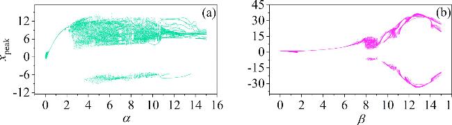
Figure 10. Bifurcation diagram of the neuron circuit corresponding to variations in α and β. The parameters are set as follows: (a) $\beta $ = 9; (b) α = 10. The other parameter: m0 = −1, m1 = 0.9, $\omega $ = 3.5, d = 1, A = 8.8, and Ic = 8. The initial conditions (0.1, 0.1, 0.1, 2). |
From figure 10, changes in parameter α lead to transitions in the membrane potentials from periodic to chaotic or from chaotic to periodic. Initially, as α increases from 0, the system exhibits periodic behavior. As this continues to rise, the system gradually transitions to a chaotic state, and with further increases in α, periodic windows re-emerge. Similarly, parameter β shows an evolution from periodic to chaotic and then back to periodic as it increases. To explore the energy modulated by α and β, we calculated the time evolution of the electric field energy in C1 and the magnetic field energy in L1 under different α and β, as shown in figure 11.
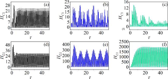
Figure 11. Time evolution of the electric field energy stored in C1 and the magnetic field energy stored in L1 corresponding to different values as: (a) α = 2, (b) α = 4, (c) α = 11; (d) β = 4, (e) β = 8.5, (f) β = 13.5. For (a)–(c) β = 9; for (d)–(f) α = 10. Other parameters: m0 = −1, m1 = 0.9, $\omega $ = 3.5, A = 8.8, and Ic = 8, d = 1. The initial conditions are set to (0.1, 0.1, 0.1, 2). |
In figure 11, as parameter α gradually increases, the system transitions between periodic and chaotic states. HC1’s amplitude decreases with increasing α, as shown in figures 11(a)–(c). Therefore, in order to reduce the energy in C1, when employing exponential gain and energy modulation to adjust parameter α, the initial value of $\alpha (\tau )$ can be set to a0 = 0.01, it is a relatively small amount. As time evolves, $\alpha $ exhibits an exponential growth trend, while the energy decreases. When the energy falls below the threshold ${\varepsilon }_{1}$, the time-varying parameter stabilizes.
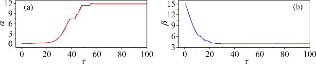
In contrast, during the increase of parameter β, the HL1’s amplitude increases. Thus, when applying the exponential gain method alongside energy modulation for adjusting β(τ), it is necessary to set a larger β0. When HL1 > ${\varepsilon }_{2}$, parameter β decreases exponentially over time, and when HL1 = ${\varepsilon }_{2}$, β remains stable. According to equation (13 ), the results of this process are illustrated in figure 12.
Figure 12. Targeted modulation of the field energy in the capacitor and inductor corresponding to their time-varying parameters $\alpha (\tau )$ and $\beta (\tau )$. The parameters: (a)${\alpha }_{0}$ = 0.01, ${\sigma }_{1}$ = 0.3, ${\varepsilon }_{1}$ = 4.5; (b)${\beta }_{0}$ = 15, ${\sigma }_{2}$ = −0.1, ${\varepsilon }_{2}$ = 30. Other parameters: m0 = −1, m1 = 0.9, $\omega $ = 3.5, A = 8.8, Ic = 8, d = 1. The initial conditions: (0.1, 0.1, 0.1, 2). |
In figure 12(a), according to equation (13 ) the initial value of the time-varying parameter α0 = 0.01, a gain coefficient ${\sigma }_{1}$ = 0.3, and a threshold ${\varepsilon }_{1}$ = 4.5, the parameter exhibits an exponential increase over time. Once HC1 ≤ ${\varepsilon }_{1}$, the parameter $\alpha $ stabilizes.
Similarly, for the time-varying parameter β(τ) with an initial value of β0 = 15, a negative gain coefficient ${\sigma }_{2}$ = −0.1, and a threshold ${\varepsilon }_{2}$ = 30, the parameter initially decreases exponentially over time. When the magnetic field energy HL1 in the inductor falls below the threshold ${\varepsilon }_{2}$, parameter $\beta $ reaches a stable value. By using this method, the targeted regulation of energy on parameters is realized.
4. Conclusion
Generalized neuron models can represent various nonlinear systems, with each model emphasizing specific physical properties of neurons. In this study, we developed a neuron model based on a double-membrane structure with magnetic and light sensitivity. This was achieved by integrating a phototube and a Josephson junction into a Chua’s circuit. We analyzed the dynamic behavior of the model and found that it can produce neuron-like firing patterns by altering the surrounding light and magnetic field. Additionally, it exhibits different energy storage modes at varying membrane potentials. We designed a parameter targeting control method by combining the principles of ‘lower energy equals higher stability’and ‘exponential gain.’Based on the principle that structure determines function, we selected structural parameters related to membrane potential and channel current in the model to verify the feasibility of this control method. Overall, the structural parameters, firing patterns, and energy storage of neurons are highly correlated.
Data availability
All data generated or analyzed during this study is included in this article.