


1. Introduction
In the study of partial differential equations (PDEs), integrable systems have been the apex in the internal waves theory [1], Bose–Einstein condensates [2, 3] and optic communications [4]. The main aim of achieving new results is to obtain soliton solutions, so many methods have been developed including the inverse scattering transformation [5], the Darboux transformation [6, 7], Bäcklund transformation [8], Lie group analysis [9], Hirota’s bilinear technique [10] and numerical approximation methods [11, 12].
Intensive research works have been invested in studying KdV, Benjamin–Ono (BO) and KP equations, which models a variety of scientific phenomena, such as the water waves with small surface tension, weakly nonlinear quasi-unidirectional waves and dust acoustic waves [13]. Recently, the multiple soliton solutions and lump solutions are unearthed by using Hirota’s bilinear technique for a (2+1)-dimensional extended Kadomtsev–Petviashvili–Benjamin–Ono (eKP–BO) equation [14]. In this paper, we concentrate on the eKP–BO equation 1 ) is a novel model for describing ocean internal solitary waves for the first time. Special cases of system (1 ) include a (2+1)-dimensional eKP equation [for a6 = 1, a7 = 1, ${a}_{1}=-\frac{{\alpha }^{2}}{4}$ and ai = 0 (i = 2, 4, 5)]
$\begin{eqnarray}\begin{array}{l}{a}_{1}{u}_{tt}+{a}_{2}{u}_{xy}+{a}_{3}{u}_{xt}+{a}_{4}{({u}^{2})}_{xx}+{a}_{5}{u}_{xxxx}\\ +\,{a}_{6}{({u}_{t}+6u{u}_{x}+{u}_{xxx})}_{x}+{a}_{7}{u}_{yy}+{a}_{8}{u}_{yt}=0,\end{array}\end{eqnarray}$
in which u = u(x, y, t) is a real differentiable function, subscripts represent partial derivatives and ai(i = 1, 2. . 8) are related to the model’s physical parameters under study. Equation ( $\begin{eqnarray}{({u}_{t}+6u{u}_{x}+{u}_{xxx})}_{x}+{u}_{yy}-\frac{{\alpha }^{2}}{4}{u}_{tt}+{a}_{3}{u}_{xt}+{a}_{8}{u}_{yt}=0,\end{eqnarray}$
which has been comprehensively studied in [15–17]. In addition, a special one is the generalized (2+1)-dimensional BO equation (for a6 = a7 = a8 = 0) $\begin{eqnarray}{a}_{1}{u}_{tt}+{a}_{2}{u}_{xy}+{a}_{3}{u}_{xt}+{a}_{4}{({u}^{2})}_{xx}+{a}_{5}{u}_{xxxx}=0,\end{eqnarray}$
which can be applied to describe the interaction of internal solitary waves in deeply stratified fluids [18–20].In the most recent period, a remarkable number of papers have focused on the in-depth investigation of the interaction waves that occur between solitons and other nonlinear waves, which has drawn increasing attention in the mathematical physics field. Researchers carry out an exhaustive investigation of interaction waves. They focus, for example, on the waves linked to the interaction between solitons and Painlevé II waves, and equally focus on those linked to the interaction between solitons and cnoidal waves, from the perspective of the nonlocal symmetry group reduction method [21–24] and the consistent tanh expansion (CTE) method [25]. The interaction waves are commonly obtained through observations in laboratory experiments, for instance, in the context of the Fermionic Quantum Plasma [26, 27]. By means of the nonlocal symmetry group reduction method that is related to the infinitesimal forms of Darboux transformation and Bäcklund transformation, a great number of new interaction waves have been discussed for different integrable models, such as variable coefficient coupled Lakshmanan–Porsezian–Daniel equation [28], modified KdV-sine Gordon equation [29, 30] and KdV-6 [31]. Furthermore, with regard to the Painlevé integrable models, the interaction solution and the n-th Bäcklund transformation have been derived from the references [32, 33], while in [34] the n-th Darboux transformation has been given. For the new model (1 ), not every PDE will give rise to integrability and interaction wave solutions, so we will be concerned with integrable and solvable problem.
The main objective of the current paper is to establish the Painlevé integrability of the extended KP–BO-type equations by employing Painlevé analysis. In the paper, we adopt a two-fold approach to propose solutions. On the one hand, we utilize the finite symmetry transformation of the extended system associated with nonlocal symmetries. On the other hand, the CTE method is employed to derive the interaction solution involving solitons and periodic waves, as well as the resonant soliton solutions. Besides, the results demonstrate that this method provides interaction solutions more conveniently compared to other methods.
The organization of the paper is delineated in the subsequent manner. In the second section, we delve into the integrability of the (2+1)-dimensional eKP–BO equation (1 ) by the Painlevé analysis. In section 3 we demonstrate the existence of the nonlocal symmetry of the eKP–BO equation (1 ) with the truncated Painlevé test. Concurrently, appropriate ancillary variables are introduced to construct the vector field of the extended system, and it is worth noting that the finite symmetry transformation is established by solving the initial value problem given by Lie’s first theorem. Within section 4 , the CTE solvability of the (2+1)-dimensional eKP–BO equation (1 ) is derived. Eventually, some analytical soliton-cnoidal interaction solutions and resonant soliton solutions are examined graphically. The final section comprises a conclusion.
2. Painlevé property for the (2+1)-Dimensional eKP–BO equation
Painlevé property is a widespread integrability property of PDEs. The familiar method for constructing the Painlevé property is proposed by Weiss, Tabor, and Carnevale (WTC) which shows that there exists a close relationship between the Painlevé property and the integrability [35]. The point of the WTC method is to propose the solution of equation (1 ) in the field of φ = 0 which is a singular manifold φ = φ(x, y, t). The solution is represented by Laurent series expansion as follows 5 ) in equation (1 ) and balancing among the most dominant terms yields $\alpha =-2,\,{u}_{0}=-\frac{{a}_{5}+{a}_{6}}{{a}_{4}+3{a}_{6}}6{\phi }_{x}^{2}$. To find the resonance point, where the coefficients of Laurent series expansion (4 ) should be arbitrary, let’s substitute the simplification expansion of equation (4 ) 1 ). Then the vanishing of the coefficient of φj−3 leads to the resonance conditions 6 ) is substituted in equation (1 ) and the coefficients of φ−6, φ−5, φ−4 and φ−3 are collected and vanished as follows. Coefficients of φ−6: 1 ) satisfies the Painlevé analysis and is integrable under the restraint $4{a}_{1}{a}_{7}-{a}_{8}^{2}=0$. Next, we proceed to solve the following integrable (2+1) eKP–BO equation
$\begin{eqnarray}u(x,y,t)={\phi }^{-\alpha }(x,y,t)\displaystyle \sum _{k=0}^{\infty }{u}_{j}(x,y,t){\phi }^{j}(x,y,t),\end{eqnarray}$
where α is negative, and uj(x, y, t)(k = 0, 1, 2. . . ) are $\begin{eqnarray}u\approx {\phi }^{\alpha }{u}_{0}.\end{eqnarray}$
Through the lead order analysis, substituting equation ( $\begin{eqnarray}u=-\frac{{a}_{5}+{a}_{6}}{{a}_{4}+3{a}_{6}}6{\phi }_{x}^{2}{\phi }^{-2}+{u}_{j}{\phi }^{j-2},\end{eqnarray}$
into equation ( $\begin{eqnarray}{\phi }_{x}^{4}(j-4)(j-5)(j-6)(j+1)({a}_{5}+{a}_{6})=0,\end{eqnarray}$
which give resonance values as $\begin{eqnarray}j=-1,\,4,\,5,\,6.\end{eqnarray}$
Apparently, the singular manifold φ(x, y, t) = 0 at j = −1 exhibits arbitrariness. Further, to obtain the arbitrariness at the other resonance points, equation ( $\begin{eqnarray}{u}_{0}=-\frac{{a}_{5}+{a}_{6}}{{a}_{4}+3{a}_{6}}6{\phi }_{x}^{2}.\end{eqnarray}$
Coefficients of φ−5: $\begin{eqnarray}{u}_{1}=\frac{{a}_{5}+{a}_{6}}{{a}_{4}+3{a}_{6}}6{\phi }_{xx}.\end{eqnarray}$
Coefficients of φ−4: $\begin{eqnarray}\begin{array}{rcl}{u}_{2} & = & \frac{1}{({a}_{4}+3{a}_{6})2{\phi }_{x}^{2}}[({a}_{3}+{a}_{6}){\phi }_{x}{\phi }_{t}+{a}_{2}{\phi }_{x}{\phi }_{y}\\ & & +(4{a}_{5}+4{a}_{6}){\phi }_{xxx}{\phi }_{x}\end{array}\end{eqnarray}$
$\begin{eqnarray}-3({a}_{5}+{a}_{6}){\phi }_{xx}^{2}+{a}_{1}{\phi }_{t}^{2}-{a}_{7}{\phi }_{y}^{2}-{a}_{8}{\phi }_{y}{\phi }_{t}].\end{eqnarray}$
Coefficients of φ−3: $\begin{eqnarray}\begin{array}{rcl}{u}_{3} & = & -\frac{1}{({a}_{4}+3{a}_{6})2{\phi }_{x}^{4}}[({a}_{5}+{a}_{6})\\ & & \times ({\phi }_{x}^{2}{\phi }_{xxxx}-4{\phi }_{x}{\phi }_{xx}{\phi }_{xxx}+3{\phi }_{xx}^{3})\\ & & +{a}_{8}({\phi }_{yt}{\phi }_{x}^{2}-{\phi }_{xx}{\phi }_{t}{\phi }_{y})+{a}_{7}({\phi }_{x}^{2}{\phi }_{xx}-{\phi }_{y}^{2}{\phi }_{xx})\\ & & +{a}_{6}({\phi }_{x}^{2}{\phi }_{xt}-{\phi }_{x}{\phi }_{t}{\phi }_{xx})\\ & & +{a}_{3}({\phi }_{x}^{2}{\phi }_{xt}-{\phi }_{xx}{\phi }_{t}{\phi }_{x})\\ & & +{a}_{2}({\phi }_{x}^{2}{\phi }_{xy}-{\phi }_{x}{\phi }_{y}{\phi }_{xx})\\ & & +{a}_{1}({\phi }_{x}^{2}{\phi }_{tt}-{\phi }_{t}^{2}{\phi }_{xx})].\end{array}\end{eqnarray}$
Coefficients of φ−2 and φ−1 are zero. Finally, by choosing a constraint $4{a}_{1}{a}_{7}-{a}_{8}^{2}=0$, the coefficient of φ0 vanishes. Without introducing any movable critical manifold, researchers can proceed to find all other coefficients of the Laurent expansion. Therefore, the eKP–BO equation ( $\begin{eqnarray}\begin{array}{l}{a}_{1}{u}_{tt}+{a}_{2}{u}_{xy}+{a}_{3}{u}_{xt}+{a}_{4}{({u}^{2})}_{xx}\\ +{a}_{5}{u}_{xxxx}+{a}_{6}{({u}_{t}+6u{u}_{x}+{u}_{xxx})}_{x}=0.\end{array}\end{eqnarray}$
under a specific case a7 = a8 = 0.3. Nonlocal symmetry
In this section, we pay attention to the symmetry integrable property of the eKP–BO equation (14 ), such as the nonlocal symmetry. Based on the truncated Painlevé test, the solution of equation (14 ) is expanded to 15 ) is substituted into the eKP–BO equation (14 ), and then the coefficients of ψ−6 and ψ−5 are made balanced, from which we derive 14 ) is put forward as 15 ) is residual symmetry, which will be crucial in the subsequent considerations [36]. It is associated with the linearized form of the eKP–BO equation (14 ) 21 ) 21 ) 21 ) evolves into 21 ), and another solution $\{\bar{u},\bar{\psi },\bar{{\rm{\Omega }}},\bar{\Upsilon }\}$, which might offer different insights, can be acquired via the finite symmetry transformation (25 ).
$\begin{eqnarray}u=\frac{{u}_{0}}{{\psi }^{2}}+\frac{{u}_{1}}{\psi }+{u}_{2},\end{eqnarray}$
where the singular manifold ψ and the analytical functions u0, u1 and u2, which pertain to the variables x, y and t, are present. Equation ( $\begin{eqnarray}{u}_{0}=-\frac{6{\psi }_{x}^{2}({a}_{5}+{a}_{6})}{{a}_{4}+3{a}_{6}},\,{u}_{1}=\frac{6{\psi }_{xx}({a}_{5}+{a}_{6})}{{a}_{4}+3{a}_{6}}.\end{eqnarray}$
Gathering the coefficients of ψ−4, the specific value of u2 is established $\begin{eqnarray}{u}_{2}=-\frac{{a}_{2}{\psi }_{y}{\psi }_{x}+{a}_{1}{\psi }_{t}^{2}+({a}_{3}+{a}_{6}){\psi }_{t}{\psi }_{x}+4({a}_{5}+{a}_{6}){\psi }_{x}{\psi }_{xxx}-3({a}_{5}+{a}_{6}){\psi }_{xx}^{2}}{(2{a}_{4}+6{a}_{6}){\psi }_{x}^{2}}.\end{eqnarray}$
Eventually, the Schwarzian formula of the eKP–BO equation ( $\begin{eqnarray}{a}_{1}{C}_{t}+({a}_{1}C+{a}_{3}+{a}_{6}){C}_{x}+{a}_{2}{K}_{x}+({a}_{5}+{a}_{6}){S}_{x}=0,\end{eqnarray}$
where under the Möbius transformation $\begin{eqnarray}\psi \to \frac{a+b\psi }{c+d\psi },\,(ad\ne bc),\end{eqnarray}$
the Schwarzian variables $S=\frac{{\psi }_{xxx}}{{\psi }_{x}}-\frac{3}{2}\frac{{\psi }_{xx}^{2}}{{\psi }_{x}^{2}}$, $C=\frac{{\psi }_{t}}{{\psi }_{x}}$ and $K=\frac{{\psi }_{y}}{{\psi }_{x}}$ retain their invariance. A very interesting class of nonlocal symmetry σ = u1 in equation ( $\begin{eqnarray}\begin{array}{l}{a}_{1}{\sigma }_{tt}+{a}_{2}{\sigma }_{xy}+{a}_{3}{\sigma }_{xt}\\ +\,{a}_{4}(2\sigma {u}_{xx}+4{u}_{x}{\sigma }_{x}+2u{\sigma }_{xx})+{a}_{5}{\sigma }_{xxxx}\\ +\,{a}_{6}({\sigma }_{xt}+12{u}_{x}{\sigma }_{x}+6\sigma {u}_{xx}+6u{\sigma }_{xx}+{\sigma }_{xxxx})=0.\end{array}\end{eqnarray}$
Subsequently, we will direct our attention to the nonlocal symmetry’s localization, which implies researchers can discover the finite symmetry transformation through Lie’s first theorem. Firstly, the extended system is presented as $\begin{eqnarray}\begin{array}{l}{a}_{1}{u}_{tt}+{a}_{2}{u}_{xy}+{a}_{3}{u}_{xt}+{a}_{4}{({u}^{2})}_{xx}+{a}_{5}{u}_{xxxx}\\ +\,{a}_{6}{({u}_{t}+6u{u}_{x}+{u}_{xxx})}_{x}=0,\\ 2({a}_{4}u+3{a}_{6}){\psi }_{x}^{2}+4({a}_{5}+{a}_{6}){\psi }_{x}{\psi }_{xxx}\\ -\,3({a}_{5}+{a}_{6}){\psi }_{xx}^{2}+{a}_{2}{\psi }_{x}{\psi }_{y}+({a}_{3}+{a}_{6}){\psi }_{x}{\psi }_{t}\\ +\,{a}_{1}{\psi }_{t}^{2}=0,\\ {\rm{\Omega }}={\psi }_{x},\,\Upsilon ={{\rm{\Omega }}}_{x}.\end{array}\end{eqnarray}$
Under the infinitesimal transformation u → u + εσ, ψ → ψ + εσψ, Ω → Ω + εσΩ and ϒ → ϒ + εσϒ, the symmetries {σ, σψ, σΩ, σϒ} are a solution of the linearized equations of the extended system ( $\begin{eqnarray}\begin{array}{l}{a}_{1}{\sigma }_{tt}+{a}_{2}{\sigma }_{xy}+{a}_{3}{\sigma }_{xt}\\ +\,2{a}_{4}(2{u}_{x}{\sigma }_{x}+\sigma {u}_{xx}+u{\sigma }_{xx})+{a}_{5}{\sigma }_{xxxx}\\ +\,{a}_{6}({\sigma }_{xt}+12{u}_{x}{\sigma }_{x}+6\sigma {u}_{xx}+6u{\sigma }_{xx}+{\sigma }_{xxxx})=0,\\ 4({a}_{5}+{a}_{6})({\sigma }_{\psi ,xxx}{\psi }_{x}^{2}-{\sigma }_{\psi ,x}{\psi }_{x}{\psi }_{xxx})\\ +\,6({a}_{5}+{a}_{6})({\sigma }_{\psi ,x}{\psi }_{xx}^{2}-{\sigma }_{\psi ,xx}{\psi }_{x}{\psi }_{xx})\\ -\,2{a}_{1}{\sigma }_{\psi ,x}{\psi }_{t}^{2}+2{a}_{1}{\sigma }_{\psi ,t}{\psi }_{x}{\psi }_{t}\\ +\,({a}_{3}+{a}_{6})({\sigma }_{\psi ,t}-{\sigma }_{\psi ,x}{\psi }_{x}{\psi }_{t})\\ +\,2\sigma ({a}_{4}+3{a}_{6}){\psi }_{x}^{3}+{a}_{2}{\sigma }_{\psi ,y}{\psi }_{x}^{2}-{a}_{2}{\sigma }_{\psi ,x}{\psi }_{y}{\psi }_{x}=0,\\ {\sigma }_{{\rm{\Omega }}}={\sigma }_{\psi ,x},\,{\sigma }_{\Upsilon }={\sigma }_{{\rm{\Omega }},x}.\end{array}\end{eqnarray}$
This amounts to saying that there exists the vectorial field of the extended system ( $\begin{eqnarray}\begin{array}{rcl}V & = & \frac{6\Upsilon ({a}_{5}+{a}_{6})}{{a}_{4}+3{a}_{6}}\frac{\partial }{\partial u}-{\psi }^{2}\frac{\partial }{\partial \psi }\\ & & -2\psi {\rm{\Omega }}\frac{\partial }{\partial {\rm{\Omega }}}-2({{\rm{\Omega }}}^{2}+\psi \Upsilon )\frac{\partial }{\partial \Upsilon }.\end{array}\end{eqnarray}$
Commencing with the Lie’s first theorem [37], the initial value problem of the extended system ( $\begin{eqnarray}\begin{array}{rcl}\frac{\,\rm{d}\,\bar{u}(\epsilon )}{\,\rm{d}\,\epsilon } & = & \frac{6({a}_{5}+{a}_{6})}{{a}_{4}+3{a}_{6}}\bar{\Upsilon }(\epsilon ),\,\bar{u}(\epsilon ){| }_{\epsilon =0}=u,\\ \frac{\,\rm{d}\,\bar{\psi }(\epsilon )}{\,\rm{d}\,\epsilon } & = & -\bar{\psi }{(\epsilon )}^{2},\,\bar{\psi }(\epsilon ){| }_{\epsilon =0}=\psi ,\\ \frac{\,\rm{d}\,\bar{{\rm{\Omega }}}(\epsilon )}{\,\rm{d}\,\epsilon } & = & -2\bar{\psi }(\epsilon )\bar{{\rm{\Omega }}}(\epsilon ),\,\bar{{\rm{\Omega }}}(\epsilon ){| }_{\epsilon =0}={\rm{\Omega }},\\ \frac{\,\rm{d}\,\bar{h}(\epsilon )}{\,\rm{d}\,\epsilon } & = & -2[\bar{{\rm{\Omega }}}{(\epsilon )}^{2}+\bar{\psi }(\epsilon )\bar{\Upsilon }(\epsilon )],\,\bar{\Upsilon }(\epsilon ){| }_{\epsilon =0}=\Upsilon \end{array}\end{eqnarray}$
the corresponding finite symmetry transformation reads $\begin{eqnarray}\begin{array}{rcl}\bar{u} & = & u-\frac{6{{\rm{\Omega }}}^{2}{\epsilon }^{2}({a}_{5}+{a}_{6})}{({a}_{4}+3{a}_{6}){(\psi \epsilon +1)}^{2}}\\ & & +\frac{6({a}_{5}+{a}_{6})\Upsilon \epsilon }{({a}_{4}+3{a}_{6})(\psi \epsilon +1)},\,\bar{\psi }=\frac{\psi }{\psi \epsilon +1},\\ \bar{{\rm{\Omega }}} & = & \frac{{\rm{\Omega }}}{{(\psi \epsilon +1)}^{2}},\,\bar{\Upsilon }=\frac{\Upsilon }{{(\psi \epsilon +1)}^{2}}-\frac{2{{\rm{\Omega }}}^{2}\epsilon }{{(\psi \epsilon +1)}^{3}}.\end{array}\end{eqnarray}$
Here, {u, ψ, Ω, ϒ} constitutes a solution of the extended system (4. CTE solvability and interaction solutions
In this part, the objective is to obtain the interaction solution of the eKP–BO equation (14 ), and one of the approaches is to establish the CTE solvability of the eKP–BO equation (14 ) by using the CTE method. Conveniently, with the application of leading order analysis, the solution of the eKP–BO equation (14 ) in truncated form is presented as 26 ) into the eKP–BO equation (14 ) and making the coefficients of ${\tanh }^{6}(w)$, ${\tanh }^{5}(w)$ and ${\tanh }^{4}(w)$ equal to zero, we achieve 14 ). Provided that the solution of equation (28 ) is given, the explicit expression for u can be concluded as 14 ) will be derived, encompassing line soliton solutions, soliton-cnoidal wave solutions and resonant soliton solutions.
$\begin{eqnarray}u={u}_{0}+{u}_{1}\tanh (w)+{u}_{2}{\tanh }^{2}(w),\end{eqnarray}$
with the analytical functions u0(x, y, t), u1(x, y, t), u2(x, y, t) and w(x, y, t). In the course of inserting equation ( $\begin{eqnarray}\begin{array}{rcl}{u}_{2} & = & -\frac{6({a}_{5}+{a}_{6}){w}_{x}^{2}}{{a}_{4}+3{a}_{6}},\,{u}_{1}=\frac{6({a}_{5}+{a}_{6}){w}_{xx}}{{a}_{4}+3{a}_{6}},\\ {u}_{0} & = & -\frac{1}{2({a}_{4}+3{a}_{6})}[({a}_{3}+{a}_{6}){w}_{x}{w}_{t}\\ & & -8({a}_{5}+{a}_{6}){w}_{x}^{4}+{a}_{1}{w}_{t}^{2}\\ & & +{a}_{2}{w}_{x}{w}_{y}+4({a}_{5}+{a}_{6}){w}_{x}{w}_{xxx}-3({a}_{5}+{a}_{6}){w}_{xx}^{2}].\end{array}\end{eqnarray}$
Finally, it can be verified that the coefficients of ${\tanh }^{2}(w)$, $\tanh (w)$ and ${\tanh }^{0}(w)$ are exactly zero by using the consistent equation $\begin{eqnarray}\begin{array}{l}4({a}_{5}+{a}_{6}){w}_{x}^{2}{w}_{xxxx}-16({a}_{5}+{a}_{6}){w}_{x}{w}_{xx}{w}_{xxx}+4{a}_{1}{w}_{tt}{w}_{x}^{2}\\ \quad +\,4({a}_{3}+{a}_{6}){w}_{x}^{2}{w}_{xt}+12({a}_{5}+{a}_{6}){w}_{xx}^{3}\\ \,-\,4[{a}_{1}{w}_{t}^{2}+({a}_{3}+{a}_{6}){w}_{x}{w}_{t}\\ \quad +\,4({a}_{5}+{a}_{6}){w}_{x}^{4}+{a}_{2}{w}_{y}{w}_{x}]{w}_{xx}+4{a}_{2}{w}_{x}^{2}{w}_{xy}=0,\end{array}\end{eqnarray}$
which is formulated from the coefficient of ${\tanh }^{3}(w)$. It is evident that this indicates the CTE solvability of the eKP–BO equation ( $\begin{eqnarray}\begin{array}{rcl}u & = & -\frac{6({a}_{5}+{a}_{6}){w}_{x}^{2}}{{a}_{4}+3{a}_{6}}{\tanh }^{2}(w)+\frac{6({a}_{5}+{a}_{6}){w}_{xx}}{{a}_{4}+3{a}_{6}}\tanh (w)\\ & & -\frac{1}{2({a}_{4}+3{a}_{6})}[({a}_{3}+{a}_{6}){w}_{x}{w}_{t}\\ & & -8({a}_{5}+{a}_{6}){w}_{x}^{4}+{a}_{1}{w}_{t}^{2}\\ & & +{a}_{2}{w}_{x}{w}_{y}+4({a}_{5}+{a}_{6}){w}_{x}{w}_{xxx}-3({a}_{5}+{a}_{6}){w}_{xx}^{2}].\end{array}\end{eqnarray}$
Subsequently, the solutions of the eKP–BO equation (Type 1: line soliton solutions
It is well-known that a commonplace line soliton solution is generated as 14 ) is presented below
$\begin{eqnarray}w={k}_{1}x+{l}_{1}y+{\omega }_{1}t,\end{eqnarray}$
and the solution of the eKP–BO equation ( $\begin{eqnarray}\begin{array}{l}u=-\frac{6{k}_{1}^{2}({a}_{6}+{a}_{5})}{{a}_{4}+3{a}_{6}}{\tanh }^{2}({\xi }_{1})\\ \,-\frac{{a}_{1}{\omega }_{1}^{2}+{l}_{1}{k}_{1}{a}_{2}+{\omega }_{1}{k}_{1}{a}_{3}+{a}_{6}{k}_{1}{\omega }_{1}-8{k}_{1}^{4}{a}_{5}+8{k}_{1}^{4}{a}_{6}}{2{k}_{1}^{2}({a}_{4}+3{a}_{6})},\end{array}\end{eqnarray}$
which ξ1 = k1x + l1y + ω1t.Type 2: soliton-cnoidal solutions
Considering the soliton-cnoidal wave, which cnoidal waves are periodic waves that are described by the Jacobi elliptic functions, the solution form is regarded as 32 ) into equation (28 ), the elliptic equation with composite variable W(ξ2) is the object of the form 14 )
$\begin{eqnarray}\begin{array}{rcl}w & = & {k}_{1}x+{l}_{1}y+{\omega }_{1}t\\ & & +W({k}_{2}x+{l}_{2}y+{\omega }_{2}t)\equiv {\xi }_{1}+W({\xi }_{2}).\end{array}\end{eqnarray}$
When substituting equation ( $\begin{eqnarray}\begin{array}{rcl}{W}_{{\xi }_{2}}^{2}({\xi }_{2}) & = & {c}_{0}+{c}_{1}W({\xi }_{2})+{c}_{2}{W}^{2}({\xi }_{2})\\ & & +{c}_{3}{W}^{3}({\xi }_{2})+{c}_{4}{W}^{4}({\xi }_{2}).\end{array}\end{eqnarray}$
Then we choose $\begin{eqnarray}\begin{array}{r}w={b}_{0}{\xi }_{2}+{\xi }_{1}+\frac{{b}_{1}}{\mu \nu }[{\rm{l}}{\rm{n}}(\mathrm{DN}-\mu \mathrm{CN})],\end{array}\end{eqnarray}$
where ξ2 = k2x + l2y + ω2t, SN stands for Jacobi elliptic function sn $(\nu {\xi }_{2},\mu )$, CN stands for Jacobi elliptic function cn $(\nu {\xi }_{2},\mu )$ and DN stands for Jacobi elliptic function dn $(\nu {\xi }_{2},\mu )$. It is feasible for one can procure the solution of the eKP–BO equation ( $\begin{eqnarray}\begin{array}{rcl}u & = & [(-3{k}_{2}^{4}{\nu }^{2}({a}_{5}+{a}_{6}){(\mu \mathrm{SN}+1)}^{2}{\tanh }^{2}({\rm{\Psi }})\\ & & +6\mu {k}_{2}^{4}{\nu }^{2}({a}_{5}+{a}_{6})\mathrm{CN}\mathrm{DN}\tanh ({\rm{\Psi }})\\ & & -3{\mu }^{2}{k}_{2}^{4}{\nu }^{2}({a}_{5}+{a}_{6}){\mathrm{SN}}^{2}+6\mu {k}_{2}^{4}{\nu }^{2}\\ & & \times ({a}_{5}+{a}_{6})\mathrm{SN}+{\nu }^{2}({\mu }^{2}+4)({a}_{5}+{a}_{6}){k}_{2}^{4}\\ & & -({a}_{2}{l}_{2}+{a}_{3}{\omega }_{2}+{a}_{6}{\omega }_{2}){k}_{2}-{a}_{1}{\omega }_{2}^{2}]\frac{1}{2{k}_{2}^{2}({a}_{4}+3{a}_{6})},\end{array}\end{eqnarray}$
where ${\rm{\Psi }}=\frac{{\mathrm{ln}}\,(\mathrm{DN}-\mu \mathrm{CN})}{2}-\frac{2y{k}_{2}^{3}({\mu }^{2}-1)({a}_{5}+{a}_{6}){\nu }^{3}+{a}_{2}{\xi }_{2}}{2{a}_{2}}$.From figure 1, people can uncover that a soliton is present on the cnoidal wave as opposed to the plane-wave background. The solution regarding the interaction between the bright soliton and cnoidal wave emerges in optical fibers. This solution describes the soliton scattering during the transport of elliptical periodic waves [38], and it also pertains to the Alfvén waves in the Fermi quantum system [26]. All calculations and visualizations were carried out using the software Maple 2023.
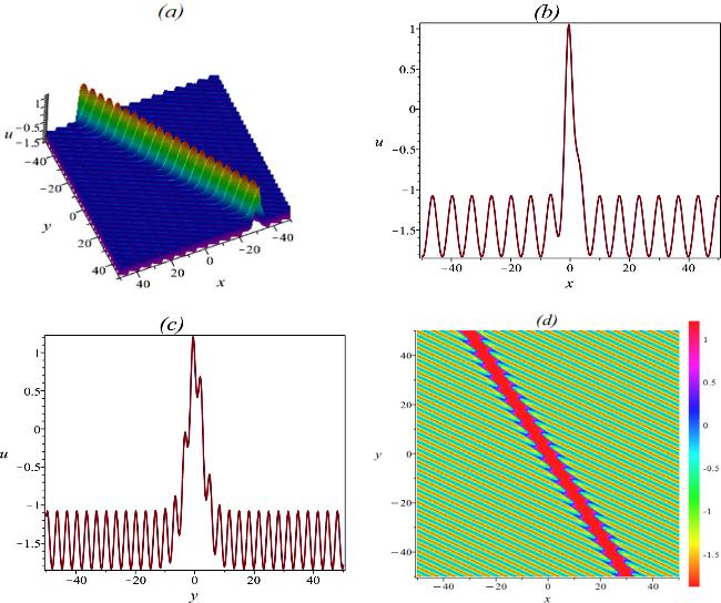
Figure 1. The bright soliton periodic wave, as represented by equation ( |
By meticulously selecting the parameters
$\begin{eqnarray}\begin{array}{l}{a}_{1}={a}_{3}={a}_{4}={a}_{5}={a}_{6}={k}_{1}={k}_{2}={l}_{2}=1,\\ {a}_{2}=2,\mu =\frac{9}{10},\nu =-1,{\omega }_{2}=\frac{1}{2},\end{array}\end{eqnarray}$
we are capable of discerning that there is a phase shift when the interaction between the soliton and the cnoidal wave occurs, as illustrated in figure 2.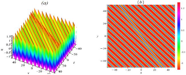
Figure 2. The phase shift phenomenon of a soliton on a cnoidal wave background expressed by equation ( |
Type 3: resonant soliton solutions
Aiming to obtain the resonant solitons, another approach is to take the following define function w14 ) by equation (29 ) with the parameter relations
$\begin{eqnarray}w={\xi }_{1}+\frac{1}{2}[{\mathrm{ln}}\,(\alpha +\beta {{\rm{e}}}^{{\xi }_{2}})],\end{eqnarray}$
we can deduce solutions of the eKP–BO equation ( $\begin{eqnarray}\begin{array}{rcl}{a}_{5} & = & -\frac{{a}_{6}{k}_{2}(4{k}_{1}+{k}_{2})}{{(2{k}_{1}+{k}_{2})}^{2}}+\frac{{a}_{1}{\omega }_{1}^{2}-12{a}_{6}{k}_{1}^{4}}{3{k}_{1}^{2}{(2{k}_{1}+{k}_{2})}^{2}}\\ & & +\frac{{a}_{1}{\omega }_{2}({k}_{1}{\omega }_{2}-2{k}_{2}{\omega }_{1})}{3{k}_{1}{k}_{2}^{2}{(2{k}_{1}+{k}_{2})}^{2}},\\ {l}_{2} & = & \frac{2{a}_{1}({k}_{1}{\omega }_{2}-{\omega }_{1}{k}_{2})(2{k}_{1}^{2}{\omega }_{2}+4{k}_{1}{k}_{2}{\omega }_{1}+2{k}_{1}{k}_{2}{\omega }_{+}{k}_{2}^{2}{\omega }_{1})}{3{k}_{1}^{2}{k}_{2}{a}_{2}(2{k}_{1}+{k}_{2})}\\ & & +\frac{({a}_{3}+{a}_{6})({k}_{1}{\omega }_{2}-{\omega }_{1}{k}_{2})}{{k}_{1}{a}_{2}}-\frac{{k}_{2}{l}_{1}}{{k}_{1}}.\end{array}\end{eqnarray}$
Figure 3 shows the resonant soliton which occurs in the maritime security and musical instruments [39, 40].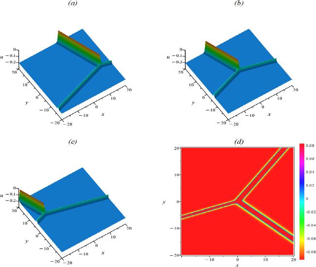
Figure 3. The resonant soliton expressed by equation ( |
5. Conclusion
In summary, the integrability property of the (2+1)-dimensional eKP–BO equation (1 ) is investigated by means of the WTC method. First of all, under the restraint a7 = a8 = 0, we obtain the Painlevé integrable equation (14 ) and its distinctive residual symmetry, which is established by utilizing the extended system (21 ). Subsequently, by utilizing the finite symmetry transformation, which we obtain by considering Lie’s first fundamental theorem to gain the initial value problem, researchers are capable of discovering several new solutions of the eKP–BO equation (14 ) from a given solution. Moreover, in accordance with the CTE method, we have obtained the consistent equation (28 ) of the eKP–BO equation (14 ), which is crucial for further analysis and understanding of the system under study. At last, we have successfully unearthed the interaction solutions of soliton-cnoidal waves, and these solutions can be explicitly constructed by the Jacobi elliptic functions. However, in the field of interaction solutions of different types of waves, there are still many unresolved issues, and these issues need to be investigated in depth in the future.