


1. Introduction
Exact or numerical solutions of NPDEs are extensively pursued in diverse areas of physical sciences, such as particle physics, condensed matter physics, plasma physics, quantum field theory, fluid dynamics, nonlinear optics, and also in mathematics, biology, chemistry, and communications [1–5]. Many powerful techniques have been invented to check the integrability of nonlinear partial differential equations (NPDEs), such as the inverse scattering [6], the bilinear or multi-linear method [7, 8], Clarkson–Kruskal’s direct method [9], the Bäcklund and Darboux transform [10], the truncated Painlevé analysis [11]. However, these methods often demand particular set of tools which require good skill or intensive computation. In addition, frequently they cannot be directly used when the equation is non-integrable.
With the advent of the new century, an increasing number of alternative methods have been proposed to obtain exact solutions of NPDEs. For example, a variational approach was introduced to effectively solve a series of variable-coefficient PDEs [12]. The exp-function method has been very successful in computing solitary wave solutions, periodic solutions, and compacton-like solutions for NPDEs [13], which is an extension of the well-known tanh-function scheme [14–16]. The method was further extended to the $({G}^{{\prime} }/G)$-expansion [17] with G = G(ξ = x − vt) satisfying an equation ${G}^{{\prime\prime} }+\lambda {G}^{{\prime} }+\mu G=0$. To accommodate more general situations, Zayed demanded that G satisfies specific nonlinear ODEs, such as ${({G}^{{\prime} })}^{2}={c}_{1}{G}^{4}+{c}_{2}{G}^{2}+{c}_{3}$ for elliptic function solutions [18], or the Riccati equation ${G}^{{\prime} }={d}_{1}+{d}_{2}{G}^{2}$ [19]. All these techniques are sub-categories of a unified scheme, the subequation method [20]. However, in their solution process, a set of nonlinear algebraic equations are invariably encountered, which are cumbersome to solve, especially with symbolic computation. Moreover, it is not easy to treat multi-soliton solutions with these techniques.
To simplify the asymptotic analysis of differential equations, a straightforward and coherent approach was introduced and is known as the renormalization group (RG) method [21, 22] which first appeared in the quantum field theory [23–26]. Considerable interest was attracted and a multitude of studies were conducted to validate the efficacy of the RG approach [27–30], which utilizes a naive perturbation expansion as its starting point and relaxes the requirement for unique intuition or experience to carry on [31]. Nevertheless, usually, the RG equation produces approximate solutions of the original equation with a much larger validity time interval than that of the perturbative expansion, which can be explained by the envelope theory or resummation technique [32]. Occasionally, the resummation happens to be exact such that an exact solution could be obtained as demonstrated in one example of Lan’s work [33]. Inspired by this, we propose an RG based polynomial approach to systematically obtain exact solutions or reduced equations for NPDEs.
Compared with traditional methods [7–11, 13, 17] mentioned above, the proposed approach does not need sophisticated analysis, focusing instead on the differential equations themselves. A large body of newly developed methods often presume the form of the solution and then substitute it into the original equation, inevitably leading to nonlinear algebraic equations to fix the parameters in the presumed form. In contrast, the current algorithm first finds a series solution of the PDE under investigation and then checks what kind of algebraic or differential equation it satisfies. As a result, only linear algebraic equations need to be solved for the undermined coefficients. The essence of the algorithm is a resummation (or renormalization) of infinite solution series with a finite number of parameters, resulting in a closed expression. It seems that the current approach is able to accommodate most variants of the subequation method [17–19] and also reduces PDEs to ODEs amenable to further analysis or computation. Moreover, a straightforward step is proposed and demonstrated to extend the new method to the computation of multi-soliton (solitary wave) solutions.
Our paper is organized as follows. In next section, the new scheme is explained in detail, including the RG approach to differential equations and the procedure for the resummation. In section 3 , four examples are used to illustrate the application of the proposed algorithm. Exact solutions including traveling waves, multi-solitons, elliptic functions are found together with the reduced equations. Finally, conclusions are drawn in section 4 .
2. The general algorithm
In this section, we explain the RG based polynomial approach and its application to the following NPDE 1 ).
$\begin{eqnarray}F(u,{u}_{t},{u}_{x},{u}_{y},\ldots ,{u}_{tt},{u}_{xt},{u}_{xx},{u}_{yy},...)=0,\end{eqnarray}$
where u = u(t, x, y, . . . ) is the state variable and t, x, y, . . . are the independent variables. F is a polynomial in u and its partial derivatives. The new approach inspired by the RG technique is illustrated in two parts. We begin by outlining the RG algorithm in solving differential equations and then demonstrate how to construct soliton solutions of PDEs (2.1. The simplified RG method
We consider the following n-dimensional differential equation 2 ). By comparing different orders of ε, we have 2 ) has been rewritten as a series of linear differential equations. We may solve them sequentially and obtain from the first one 5 ) into the second equation of (4 ), we get
$\begin{eqnarray}\dot{X}=LX+\epsilon N(X),\end{eqnarray}$
where $X={({x}_{1},{x}_{2},\ldots ,{x}_{n})}^{\top }$ denotes the state variable and L = diag(l1, l2, …, ln) is an n × n diagonal matrix, where ${\{{l}_{i}\}}_{i=1,2,\ldots ,n}$ are eigenvalues of L. N(x) is the nonlinear term. ε is a small parameter which controls the size of nonlinearity. To start the perturbation calculation, we expand the solution to an infinite series $\begin{eqnarray}X={X}_{1}+\epsilon {X}_{2}+{\epsilon }^{2}{X}_{3}+...,\end{eqnarray}$
and substitute it into ( $\begin{eqnarray}\begin{array}{l}\dot{{X}_{1}}\,=\,L{X}_{1}\\ \dot{{X}_{2}}\,=\,L{X}_{2}+N({X}_{1})\\ \,....\end{array}\end{eqnarray}$
Here the nonlinear differential equation ( $\begin{eqnarray}{X}_{1}(t,{t}_{0})=A{\,\rm{e}\,}^{L(t-{t}_{0})},\end{eqnarray}$
where t0 is the initial time and $A=A({t}_{0})\,={[{A}_{1}({t}_{0}),{A}_{2}({t}_{0}),\ldots ,{A}_{n}({t}_{0})]}^{\top }$ is a constant vector representing the initial positions. Substituting ( $\begin{eqnarray}\begin{array}{rcl}{X}_{2}(t,{t}_{0}) & = & \tilde{A}{\,\rm{e}\,}^{L(t-{t}_{0})}+{\,\rm{e}\,}^{L(t-{t}_{0})}\\ & & \times \,{\displaystyle \int }_{{t}_{0}}^{t}{\,\rm{e}\,}^{-L(\tau -{t}_{0})}N[A{\,\rm{e}\,}^{L(\tau -{t}_{0})}]\,\rm{d}\,\tau ,\end{array}\end{eqnarray}$
where $\tilde{A}$ is the undetermined constant vector, which will be chosen properly later on.In some cases, after integrating equation (6 ) or other high order equations in equation (4 ), resonance terms (t − t0) may appear, which unbounded when t → ∞. The approximation $X=\tilde{X}[t;{t}_{0},A({t}_{0})]$ becomes invalid beyond the time scale of O(ε). Therefore, Chen and Goldenfeld et al [21, 22] introduced an intermediate time τ between t and t0 to carry out the renormalization group calculation to extend the validity region, which could be much simplified [33, 34] with an alternative RG equation 7 ) states that the position $\tilde{X}[t;{t}_{0},A({t}_{0})]$ at t should be fixed if we change the initial parameters t0 and A(t0) in a proper way. The condition t = t0 in (7 ) is used to accommodate the fact that $\tilde{X}(t;{t}_{0},A({t}_{0}))$ is an approximate solution. If $\tilde{X}(t;{t}_{0},A({t}_{0}))$ is exact, it is not imperative to enforce t = t0. When the equation does not contain resonance terms, the solution $\tilde{X}(t;{t}_{0},A({t}_{0}))$ only contains exponential functions.
$\begin{eqnarray}\frac{\,\rm{d}\,\tilde{X}[t;{t}_{0},A({t}_{0})]}{\,\rm{d}\,{t}_{0}}{| }_{t={t}_{0}}=0,\end{eqnarray}$
without the introduction of τ. The RG equation (To see how the above steps work, we use the classical KdV equation 8 ) and comparing different orders of ε, one gets a set of linear PDEs 9a ) is ${u}_{1}={\sum }_{i=1}^{n}{A}_{i}{\,\rm{e}\,}^{{k}_{i}(x-{x}_{0})+{\omega }_{i}(t-{t}_{0})}$, where ${w}_{i}=-{k}_{i}^{3}-c{k}_{i}$ and Ai are constants depending on the initial position and time x0, t0. Here, we have chosen n modes for calculation. Substituting the solution u1 into equation (9b ), we have 9b ). With this operation repeated, the higher order terms such as u3, u4, ... could be sequentially obtained. The approximation becomes 10 ) reduces to a polynomial 1 ).
$\begin{eqnarray}{u}_{t}+u{u}_{x}+{u}_{xxx}=0.\end{eqnarray}$
Substituting the naive expansion u = c + εu1 + ε2u2 + . . . into equation ( $\begin{eqnarray}{u}_{1t}+c{u}_{1x}+{u}_{1xxx}=0,\end{eqnarray}$
$\begin{eqnarray}{u}_{2t}+c{u}_{2x}+{u}_{2xxx}+{u}_{1}{u}_{1x}=0,\end{eqnarray}$
$\begin{eqnarray}\begin{array}{l}{u}_{3t}+c{u}_{3x}+{u}_{3xxx}+{u}_{2}{u}_{1x}+{u}_{2x}{u}_{1}=0,...,\end{array}\end{eqnarray}$
where c is an arbitrary constant. In the following, different values of c may yield distinct results. The solution of equation ( $\begin{eqnarray*}{u}_{2}=\displaystyle \sum _{i=1}^{n}\displaystyle \sum _{j=1}^{n}{q}_{ij}{k}_{j}{A}_{i}{A}_{j}{\,\rm{e}\,}^{({k}_{i}+{k}_{j})(x-{x}_{0})+({\omega }_{i}+{\omega }_{j})(t-{t}_{0})},\end{eqnarray*}$
where qij’s values can be computed by integrating the linear differential equation equation ( $\begin{eqnarray}\begin{array}{rcl}u & = & c+\epsilon \displaystyle \sum _{i=1}^{n}{A}_{i}{\,\rm{e}\,}^{{k}_{i}(x-{x}_{0})+{\omega }_{i}(t-{t}_{0})}\\ & & +{\epsilon }^{2}\displaystyle \sum _{i=1}^{n}\displaystyle \sum _{j=1}^{n}{q}_{ij}{k}_{j}{A}_{i}{A}_{j}{\,\rm{e}\,}^{({k}_{i}+{k}_{j})(x-{x}_{0})+({\omega }_{i}+{\omega }_{j})(t-{t}_{0})}\\ & & +{\epsilon }^{3}(...)+....\end{array}\end{eqnarray}$
Applying the RG equation $\frac{\rm{d}\,u}{\,\rm{d}{t}_{0}}{| }_{t={t}_{0},x={x}_{0}}=0$ and $\frac{\rm{d}\,u}{\,\rm{d}{x}_{0}}{| }_{t={t}_{0},x={x}_{0}}=0$, we obtain $\frac{\partial {\tilde{A}}_{i}}{\partial {x}_{0}}={k}_{i}{\tilde{A}}_{i}$ and $\frac{\partial {\tilde{A}}_{i}}{\partial {t}_{0}}={\omega }_{i}{\tilde{A}}_{i}$. Altogether, the solution ${\tilde{A}}_{i}={C}_{i}{\,\rm{e}\,}^{{k}_{i}{x}_{0}+{\omega }_{i}{t}_{0}}$ where ${\{{C}_{i}\}}_{i=1,\ldots ,n}$ are integration constants. By setting t = t0, x = x0, the expansion ( $\begin{eqnarray}u=c+\epsilon \displaystyle \sum _{i=1}^{n}{A}_{i}+{\epsilon }^{2}\displaystyle \sum _{i=1}^{n}\displaystyle \sum _{j=1}^{n}{q}_{ij}{k}_{j}{A}_{i}{A}_{j}+{\epsilon }^{3}(...)+....\end{eqnarray}$
If we study m-soliton solutions to the KdV equation, we may set n = m. It is worth mentioning that the RG steps described above are also valid for the general NPDE (2.2. The procedure for finding the exact solutions of general PDE
For general NPDE (1 ), once the approximation equation (11 ) is obtained, it is very convenient to check what kind of simple algebraic or differential equations that it satisfies. For example, we may multiply both sides of equation (11 ) by a trial polynomial P of ${\{{A}_{i}\}}_{i=1,\cdots \,{,}n}$ 1 ) is obtained in a rational form 12 ) increases substantially with extra solitons chipping in. Consequently, when constructing the polynomial representation for multiple solitons, we will renormalize the parameters A based on the one-soliton framework to reduce the number of coefficients, which will be elaborated in the applications below.
$\begin{eqnarray}P=\epsilon {a}_{0}+{\epsilon }^{2}\displaystyle \sum _{i=1}^{n}{a}_{i}{A}_{i}+{\epsilon }^{3}\displaystyle \sum _{i=1}^{n}\displaystyle \sum _{j=1}^{n}{b}_{ij}{A}_{i}{A}_{j}+{\epsilon }^{3}(...)+...\end{eqnarray}$
to see whether the series becomes finite or not, where ${\{{a}_{i},{b}_{ij}\}}_{i,j=1,2,\ldots ,n}$ are undetermined coefficients. If the product $\begin{eqnarray}\begin{array}{rcl}Pu & = & \epsilon {a}_{0}c+{\epsilon }^{2}\displaystyle \sum _{i=1}^{n}({a}_{0}+{a}_{i}c){A}_{i}+{\epsilon }^{3}\displaystyle \sum _{i=1}^{n}\displaystyle \sum _{j=1}^{n}(c{b}_{ij}\\ & & +{a}_{0}{q}_{ij}{k}_{j}+{a}_{i}){A}_{i}{A}_{j}+{\epsilon }^{4}(...)+....\end{array}\end{eqnarray}$
is a finite series, say, terminated at εh, we may set the coefficients of high order terms at ${\{{\epsilon }^{j}\}}_{j=h,h+1,\ldots ,n}$ to zero, in order to get the proper coefficients ${\{{a}_{i},{b}_{ij}\}}_{i,j=1,2,\ldots ,n}$. Then, the n-solitory wave solution for the general NPDE ( $\begin{eqnarray}\begin{array}{rcl}u & = & (\epsilon {a}_{0}c+{\epsilon }^{2}\displaystyle \sum _{i=1}^{n}({a}_{0}+{a}_{i}c){A}_{i}+{\epsilon }^{3}\displaystyle \sum _{i=1}^{n}\displaystyle \sum _{j=1}^{n}(c{b}_{ij}\\ & & +{a}_{0}{q}_{ij}{k}_{j}+{a}_{i}){A}_{i}{A}_{j}+{\epsilon }^{h-1}(...))/p.\end{array}\end{eqnarray}$
The most interesting feature of the current procedure is that the undetermined coefficients ${\{{a}_{i},{b}_{ij}\}}_{i,j=1,2,\ldots ,n}$ satisfy a set of linear algebraic equations in contrast to many existing techniques [13, 18, 19, 35]. It is expected that the number of coefficients in the polynomial equation (On the other hand, simple differential equations could also be derived that are satisfied by our approximation (10 ). Similar to what has been done above, if these equations are valid up to high orders, it is very likely that the exact solution also satisfies them. Still, only a linear set of algebraic equations need to be solved, which seems more convenient than many popular methods based on subequations [13, 14, 16–18]. In the following, as an example, we list the steps to reduce PDE (1 ) to a second-order ODE. For a PDE with constant coefficients, we introduce a new variable θ = kx + ry + . . . + ωt and consider the traveling wave solution. With a similar procedure leading to (8 )–(11 ), we get the approximation of equation (1 ) 1 ) satisfies the following second-order equation 15 ) into equation (16 ) and equating the coefficients of different orders of A to zero, as expected, we get a set of linear algebraic equations that the coefficients ${\{{b}_{i}\}}_{i=0,1,2,3}$ satisfy. Therefore, these coefficients may be obtained by solving the linear equations from low orders of A and then substituted into equations at high orders to check their validity. Sometimes, this procedure may even be used in variable-coefficient PDEs to derive exact solutions as will be shown below.
$\begin{eqnarray}\begin{array}{rcl}u & = & c+\epsilon A+{\epsilon }^{2}{q}_{1}{A}^{2}+{\epsilon }^{3}{q}_{2}{A}^{3}+{\epsilon }^{4}{q}_{3}{A}^{4}+...,\\ {u}_{\theta \theta } & = & \epsilon A+4{\epsilon }^{2}{q}_{1}{A}^{2}+9{\epsilon }^{3}{q}_{2}{A}^{3}+16{\epsilon }^{4}{q}_{3}{A}^{4}+...,\end{array}\end{eqnarray}$
where a = eθ and ${\{{q}_{i}\}}_{i=1,2,...}$ are known coefficients. Next, we assume that the approximation ( $\begin{eqnarray}{u}_{\theta \theta }+{b}_{0}+\epsilon {b}_{1}u+{\epsilon }^{2}{b}_{2}{u}^{2}+{\epsilon }^{3}{b}_{3}{u}^{3}=0,\end{eqnarray}$
where ${\{{b}_{i}\}}_{i=0,1,2,3}$ are four undetermined coefficients. Substituting expansion (3. Applications
In this section, we use four examples to illustrate how the polynomial method based on the RG scheme is employed to find one- and two-soliton (solitary wave) solutions of NPDEs, including the generalized Hirota–Satsuma–Ito equation, one typical 5th-order evolution equation, the variable-coefficient modified Kadomatsey–Petviashvilli equation, and the Calogero equation. In the first example, we provide detailed application steps of the polynomial method to real situations. In the second example, a new exact solution is derived with the current approach. It can also be used to treat NPDEs with variable coefficients as demonstrated in the third example. In the final application, we get reduced equations based on the above procedure, which may possess solutions that could not pass the Painlevé test.
3.1. Application. A: Hirota–Satsuma–Ito equation
We first focus on the generalized Hirota–Satsuma–Ito (g-HSI) equation that describes the unidirectional propagation of shallow water waves [36], which has been investigated extensively in recent years. N-soliton solutions for the (2 + 1)-dimensional g-HSI equation were derived with the Hirota’s direct method [37], revealing various localized wave interaction along with their behavior upon parameter change. Zhou and Manukure [38] computed new class of solutions for the g-HSI equation with the help of the Hirota’s bilinear method and nonlinear superposition principle. In the following, we rederive the one- and two-soliton solutions of the g-HSI equation to illustrate the effectiveness of our new approach. Then, elliptic function solutions to the g-HSI equation are derived from a reduced second-order equations obtained with the current scheme.
The (2 + 1)-dimensional g-HSI equation is
$\begin{eqnarray}\left\{\begin{array}{ll}{v}_{t} & =\,-{u}_{xxt}-3{(uw)}_{x}-\alpha {u}_{x},\\ {u}_{y} & =\,{v}_{x},\\ {u}_{t} & =\,{w}_{x},\end{array}\right.\end{eqnarray}$
where α is a non-zero real constant, u = u(x, y, t) is the physical field while v = v(x, y, t) and w = w(x, y, t) are the potentials of u(x, y, t) derivatives. The equation is nonlinear with three dependent variables and non-uniform structures, so its solution is nontrivial. Next, we show how to derive the one- and two-soliton as well as the elliptic function solutions with the polynomial method base on the RG procedure.3.1.1. The one-soliton solution
We write the perturbative expansion 17 ). With the standard steps (8 )–(10 ), we have the following approximation of traveling wave solutions 19 ) is simplified to the following polynomial 20 ). For that purpose, we try a polynomial P1 of fifth order 20 ) gives us 22 ) should be zero. With this consideration, we try truncating equation (22 ) from the fourth order, i.e., taking f4 = 0, f5 = 0, ..., which fixes the coefficients a0 = 1, ${a}_{1}=\frac{1}{{k}^{2}}$, ${a}_{2}=\frac{1}{4{k}^{4}}$, a3 = 0, a4 = 0, a5 = 0. So, the coefficients ai are computed by solving a set of linear algebraic functions. In fact, the truncation of the series (22 ) could be started from any order higher than three without changing the result since all the coefficients of higher orders are zero. Of course, we have not given a proof for this statement. However, after the one-soliton solution is written down according to equation (22 ) 17 ), we get $v=\frac{4{k}^{4}ar}{k{(a+2{k}^{2})}^{2}}$ and $w=-\frac{4{k}^{4}a{k}^{2}\alpha }{(3c{k}^{2}+{k}^{4}+rk){(a+2{k}^{2})}^{2}}$. One easily finds that the symbol of the potential w is proportional to the non-zero real constant α. Furthermore, the solution (24 ) can be rewritten as $u=c+\frac{{k}^{2}}{2}{{\rm{{\rm{sech}} }}}^{2}(\theta )$ with C = 2k2, giving an amplitude of $\frac{{k}^{2}}{2}$, and its envelop velocities along x-axis and y-axis of $\frac{k\alpha }{3ck+{k}^{3}+r}$ and $\frac{{k}^{2}\alpha }{(3ck+{k}^{3}+r)r}$, respectively. The profiles of the state u and its potentials v and w at t = 0 are depicted in figure 1 with k = 3, r = 1, c = 0, and α = − 2. It is easy to see that u and v are bell-shaped solitons, while the potential w is anti-bell-shaped one-soliton. Nevertheless, if we take α = 2 while keeping the other parameters unchanged, w will become bell-shaped.
$\begin{eqnarray}u=c+\epsilon {u}_{1}+{\epsilon }^{2}{u}_{2}+{\epsilon }^{3}{u}_{3}+...,\end{eqnarray}$
where c is a constant, which is also a solution of equation ( $\begin{eqnarray}u=c+\epsilon a{\rm{e}\,}^{\theta }+{\epsilon }^{2}{p}_{1}{a}^{2}{\rm{e}}^{2\theta }+{\epsilon }^{3}{p}_{2}{a}^{3}{\,\rm{e}}^{3\theta }+...,\end{eqnarray}$
where θ = k(x − x0) + r(y − y0) + s(t − t0) and $s=-\frac{{k}^{2}\alpha }{3ck+{k}^{3}+r}$, ${p}_{1}=-\frac{1}{{k}^{2}}$, ${p}_{2}=-\frac{3{p}_{1}}{4{k}^{2}}$, .... With the RG equation $\frac{\rm{d}\,u}{\rm{d}{x}_{0}}{| }_{t={t}_{0},x={x}_{0},y={y}_{0}}=0,\frac{\rm{d}u}{\rm{d}{y}_{0}}{| }_{t={t}_{0},x={x}_{0},y={y}_{0}}=0,\frac{\rm{d}u}{\,\rm{d}{t}_{0}}{| }_{t={t}_{0},x={x}_{0},y={y}_{0}}=0,$ we obtain a = Ceθ, where C is an arbitrary constant. With the substitution t = t0, x = x0, y = y0, the expansion ( $\begin{eqnarray}u=c+\epsilon a+{\epsilon }^{2}{p}_{1}{a}^{2}+{\epsilon }^{3}{p}_{2}{a}^{3}....\end{eqnarray}$
To get a closed-form solution, we need to resum the series in equation ( $\begin{eqnarray}{P}_{1}={a}_{0}+{a}_{1}a+{a}_{2}{a}^{2}+{a}_{3}{a}^{3}+{a}_{4}{a}^{4}+{a}_{5}{a}^{5},\end{eqnarray}$
where ${\{{a}_{i}\}}_{i=0,1,2,3,4,5}$ are unknown coefficients to be determined. Multiplying P1 on the both sides of equation ( $\begin{eqnarray}{P}_{1}u={a}_{0}c+{f}_{1}a+{f}_{2}{a}^{2}+{f}_{3}{a}^{3}+{f}_{4}{a}^{4}+{f}_{5}{a}^{5}...,\end{eqnarray}$
where $\begin{eqnarray}\begin{array}{rcl}{f}_{1} & = & {a}_{1}c+{a}_{0},\\ {f}_{2} & = & {a}_{2}c+{a}_{1}+{a}_{0}{p}_{1},\\ {f}_{3} & = & {a}_{3}c+{a}_{2}+{a}_{1}{p}_{1}+{a}_{0}{p}_{2},\\ {f}_{4} & = & {a}_{4}c+{a}_{3}+{a}_{2}{p}_{1}+{a}_{1}{p}_{1}+{a}_{0}{p}_{3},\\ {f}_{5} & = & {a}_{5}c+{a}_{4}+{a}_{3}{p}_{1}+{a}_{2}{p}_{1}+{a}_{1}{p}_{3}+{a}_{0}{p}_{4},\\ .... & & \end{array}\end{eqnarray}$
For a closed-form solution, the coefficients of the higher order terms of a in equation ( $\begin{eqnarray}u=\frac{4c{k}^{4}+4{k}^{2}(c+{k}^{2})a+c{a}^{2}}{{(a+2{k}^{2})}^{2}},\end{eqnarray}$
where a = Ceθ, $\theta =kx+ry-\frac{{k}^{2}\alpha }{3ck+{k}^{3}+r}t$, it is always easy to check its validity by a direct substitution into the original equation. From equation (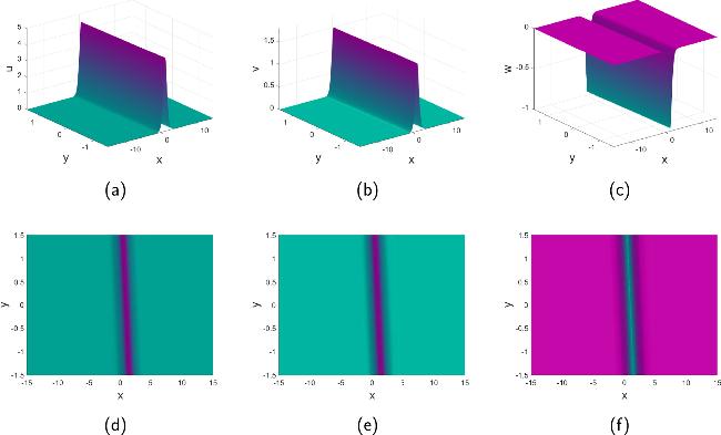
Figure 1. One-soliton solution u, v and w of equation ( |
3.1.2. The two-soliton solution
By repeating the RG procedure (8 )–(11 ), we derive the two-soliton type of expansion (25 ) for PDE (17 ) 70 ) of appendix A.1 . Following a similar line as before, we obtain the two-soliton solutions of equation (17 ) by designing the polynomial P2 as shown below 26 ) truly necessary? In other words, is it possible to determine some unknowns in advance to simplify the coefficient equations? In general, it is hard to carry out this simplification. But for soliton solutions, we have extra information, the solitons satisfy a certain kind of nonlinear superposition principle. The multi-soliton solution could be reduced to solution with fewer solitons, which put constraints on the form of the denominator P2.
$\begin{eqnarray}\begin{array}{lll}u & = & c+\epsilon (a+b)+{\epsilon }^{2}({p}_{11}{a}^{2}+{p}_{12}{b}^{2}+{p}_{13}ab)+{\epsilon }^{3}({p}_{21}{a}^{3}\\ & & +{p}_{22}{b}^{3}+{p}_{23}{a}^{2}b+{p}_{24}a{b}^{2})+{\epsilon }^{4}(...)+....\end{array}\end{eqnarray}$
with two variables $a={C}_{1}{\,\rm{e}\,}^{{\theta }_{1}}$ and $b={C}_{2}{\,\rm{e}\,}^{{\theta }_{2}}$, where C1, C2 are arbitrary constants. θi = ki(x − x0) + ri(y − y0) + si(t − t0), ${\left\{{s}_{i}=-\frac{{k}_{i}^{2}\alpha }{3c{k}_{i}+{k}_{i}^{3}+{r}_{i}}\right\}}_{i=1,2}$, and ${\{{p}_{ij}\}}_{i=1,2,...}$ are known coefficients, displayed in equation ( $\begin{eqnarray}\begin{array}{rcl}{P}_{2} & = & {c}_{0}+\epsilon ({c}_{1}a+{c}_{2}b)+{\epsilon }^{2}({c}_{3}{a}^{2}+{c}_{4}{b}^{2}+{c}_{5}ab)\\ & & +{\epsilon }^{3}({c}_{6}{a}^{3}+{c}_{7}{b}^{3}+{c}_{8}{a}^{2}b+{c}_{9}a{b}^{2})+{\epsilon }^{4}({c}_{10}{a}^{4}\\ & & +{c}_{11}{b}^{4}+{c}_{12}{a}^{3}b+{c}_{13}a{b}^{3}+{c}_{14}{a}^{2}{b}^{2})+{\epsilon }^{5}(...)+...,\end{array}\end{eqnarray}$
where ${\{{c}_{i}\}}_{i=0,1,2,...}$ are coefficients to be determined. Although they satisfy a set of linear equations, it may not be so easy to solve this linear set with symbolic computation if system parameters are involved in these equations. Is every term in equation (With the above consideration, we next renormalize the variable a depicted in one-soliton solution (24 ) to a → d1a + d2b + d3ab + d4a2b + d5ab2 + d6a3b + d7ab3 + d8a2b2 + . . . , with ${\{{d}_{i}\}}_{i=1,2,...}$ being coefficients. Substituting it into the one-soliton solution (24 ), we get a simplified form P2 = c0 + c1a + c2b + c3a2 + c4b2 + c5ab + c6a2b + c7ab2 + c8a2b2 + . . . , with the coefficients ${\{{c}_{i}\}}_{i=1,2,...}$ to be determined below.
Multiplying both sides of equation (25 ) with the simplified P2 and equating high orders of ε in the product to zero, we obtain the two-soliton solution 71 ) and (72 ) of Appendix A.2 . By taking a = 0 or b = 0, the two-soliton solution (27 ) reduces to the one-soliton solution (24 ) as stated before.
$\begin{eqnarray}u=\frac{{n}_{1}+{n}_{2}a+{n}_{3}b+{n}_{4}{a}^{2}+{n}_{5}{b}^{2}+{n}_{6}ab+{n}_{7}{a}^{2}b+{n}_{8}a{b}^{2}+{n}_{9}{a}^{2}{b}^{2}}{1+{m}_{1}a+{m}_{2}b+{m}_{3}{a}^{2}+{m}_{4}{b}^{2}+{m}_{5}ab+{m}_{6}{a}^{2}b+{m}_{7}a{b}^{2}+{m}_{8}{a}^{2}{b}^{2}},\end{eqnarray}$
where $a={C}_{1}{\,\rm{e}\,}^{{\theta }_{1}}$, $b={C}_{2}{\,\rm{e}\,}^{{\theta }_{2}}$, with ${\{{n}_{i}\}}_{i=1,2,\ldots ,8}$, ${\{{m}_{i}\}}_{i=1,2,\ldots ,8}$, shown in equations (As we have mentioned above, the soliton solutions (24 ) and (27 ) of system (17 ) were obtained with the well-known Hirota bilinear method [37], where the transformation $u=2{({\mathrm{ln}}\,f)}_{xx}$ was used to convert the origin PDE to a bilinear equation. In contrast, the current approach does not need such a transform which sometimes may not be so obvious. Due to the complexity , we do not present the explicit expressions for the potentials v and w. The state variable u with parameters k1 = 3, k2 = 4, r1 = 5, r2 = 8, α = − 2, and c = 0 at t = 0 is plotted in figure 2, from which we find that the solution equation (27 ) is a two-bell-shaped soliton.
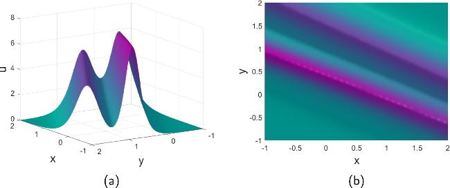
Figure 2. Two-soliton solution ( |
Next, we discuss the periodic structures that the solution (27 ) may exhibit. Taking k1 = k2 = 1/2, ${r}_{1}=1/\sqrt{2}\,\rm{i}\,$, ${r}_{2}=-1/\sqrt{2}\,\rm{i}\,$, α = − 2, and c = 0 at t = 0, one may obtain the y-periodic soliton as shown in figure 3. Notably, the dispersions r1 and r2 are a conjugate pure imaginary pair in this case. If we keep the other parameters fixed and assign new values ${r}_{1}=1+1/\sqrt{2}\,\rm{i}\,$ and ${r}_{2}=1-1/\sqrt{2}\,\rm{i}\,$, the corresponding soliton is presented in figure 4, where the wave-vector is tilting in the (x, y)-plane. However, periodic solution of more general types may be obtained with the new method.
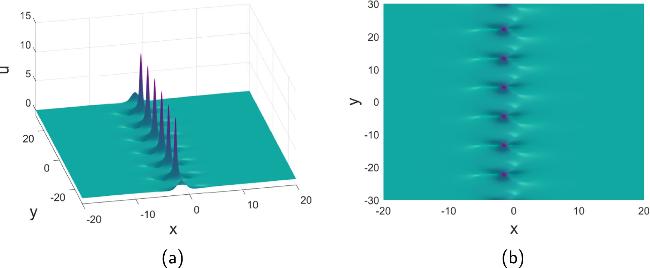
Figure 3. The y-periodic soliton solution ( |
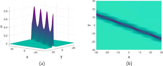
Figure 4. The (x, y)-periodic soliton solution ( |
3.1.3. The Jacobi elliptic function solution
In this sub-section, we extend our method to derive an elliptic function solution to equation (17 ).
The standard elliptic function satisfies 20 ) and its second derivative uθθ = εa + 4ε2p1a2 + 9ε3p2a3. . . into equation (28 ) and comparing coefficients of different orders of a, we have 17 ) 31 ) has the solution $u=\frac{4{k}^{4}C{\,\rm{e}\,}^{\theta }}{{(2{k}^{2}+C{\,\rm{e}\,}^{\theta })}^{2}}$ while equation (32 ) has the solution $u=\frac{4{k}^{4}+4({k}^{4}+{k}^{2})C{\rm{e}\,}^{\theta }+{C}^{2}{\,\rm{e}}^{\theta }}{{(2{k}^{2}+C{\,\rm{e}\,}^{\theta })}^{2}}$, both in an exponential form. Nevertheless, equation (32 ) also possesses a Jacobi elliptic function solution 32 ) hinges on the value of k. If we set k = 1.8*i (here,i2 = − 1), r = 0.01, and α = 1/2 at t = 0, the solution (33 ) becomes x-periodic, which is plotted in figure 5. Now, the profile turns sharp near the peak and broad at the trough, typical of nonlinear waves.
$\begin{eqnarray}{u}_{\theta \theta }+{b}_{1}+{b}_{2}u+{b}_{3}{u}^{2}+{b}_{4}{u}^{3}=0,\end{eqnarray}$
where ${\{{b}_{i}\}}_{i=1,2,3,4}$ are undetermined coefficients. Substituting the expansion ( $\begin{eqnarray}\begin{array}{l}{a}^{0}\to {b}_{1}+c{b}_{2}+{c}^{2}{b}_{3}+{c}^{3}{b}_{4}=0,\\ {a}^{1}\to 1+{b}_{2}+2c{b}_{3}+3{c}^{2}{b}_{4}=0,\\ {a}^{2}\to {b}_{3}+3c{b}_{4}-\frac{4+{b}_{2}+2c{b}_{3}+3{c}^{2}{b}_{4}}{{k}^{2}}=0,\\ ....\end{array}\end{eqnarray}$
It is evident that the coefficients satisfy a system of linear algebraic equations, giving ${b}_{1}=c+\frac{3{c}^{2}}{{k}^{2}}$, ${b}_{2}=-1-\frac{6c}{{k}^{2}}$, ${b}_{3}=\frac{3}{{k}^{2}}$, and b4 = 0. It is easy to check that with these values, the coefficients of higher orders are also zero. Therefore, we arrive at the reduced equation of PDE ( $\begin{eqnarray}{u}_{\theta \theta }+\frac{c{k}^{2}+3{c}^{2}}{{k}^{2}}-\frac{{k}^{2}+6c}{{k}^{2}}u+\frac{3}{{k}^{2}}{u}^{2}=0.\end{eqnarray}$
Taking c = 0 or c = 1 leads to two different equations $\begin{eqnarray}{u}_{\theta \theta }-u+\frac{3}{{k}^{2}}{u}^{2}=0,\end{eqnarray}$
$\begin{eqnarray}{u}_{\theta \theta }+\frac{{k}^{2}+3}{{k}^{2}}-\frac{{k}^{2}+6}{{k}^{2}}u+\frac{3}{{k}^{2}}{u}^{2}=0.\end{eqnarray}$
Equation ( $\begin{eqnarray}u=A{{\rm{sn}}}^{2}(B\theta ,m),\end{eqnarray}$
where $\theta =kx+ry-\frac{{k}^{2}\alpha }{3ck+{k}^{3}+r}t$ and the symbol ${\unicode{x0201C}}{\rm{sn}}\mbox{''}$ denotes the well-known Jacobi elliptic function, with $\begin{eqnarray*}\begin{array}{rcl}A & = & \frac{1}{4}(6+{k}^{2}+\sqrt{{k}^{4}-4{k}^{2}-12}),\\ B & = & \frac{\sqrt{6+{k}^{2}-\sqrt{{k}^{4}-4{k}^{2}-12}}}{2\sqrt{2}k\,\rm{i}\,},\\ m & = & \frac{{k}^{4}+6(2+\sqrt{{k}^{4}-4{k}^{2}-12})+{k}^{2}(4+\sqrt{{k}^{4}-4{k}^{2}-12})}{8(3+{k}^{2})}.\end{array}\end{eqnarray*}$
The dynamics of equation (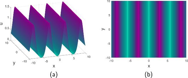
Figure 5. The elliptic function solution ( |
In this application, we demonstrate how the one- and two-soliton solutions are computed with the polynomial method based on the RG scheme. In the study of the two-soliton solutions, we renormalized the variable a in the one-soliton solution to simplify the form of the auxiliary polynomial, which significantly simplifies the computation. A Jacobi elliptic function solution has is also derived although the starting point is a series expansion in exponential functions. The periodic solution yielded by the current approach seems distinct from what is reported in [37]. Below, the same scheme will be applied to different examples for solutions of elliptic function type.
3.2. Application. B: The general class of 5th-order evolution equation
In this application, we apply the new method to a well-known general class of 5th-order evolution equation [39] below
$\begin{eqnarray}{u}_{t}+\delta u{u}_{xxx}+\lambda {u}_{x}{u}_{xx}+\mu {u}^{2}{u}_{x}+{u}_{xxxxx}=0,\end{eqnarray}$
where δ, λ, and μ are arbitrary real parameters.This equation can be transformed into numerous equations with distinct properties as the parameters δ, λ, and μ take different values. For example, when δ = 10, λ = 20, and μ = 30, equation (34 ) is called Lax equation; it is also noted as Sawada–Kotera (SK) equation [40, 41] at δ = − 15, λ = − 15, and μ = 45 or δ = 5, λ = 5, and μ = 5. These two equations are fully integrable and have N-soliton solutions. By choosing δ = 10, λ = 25, and μ = 20 or δ = − 15, λ = − 75/2, and μ = 45, one gets the well-known Kaup–Kupershmidt (KK) equation. In the case of δ = 10, λ = 25, and μ = 20, the N-soliton solutions are not known [39], even though it has been proven to be integrable [42]; furthermore, the KK equation cannot be rewritten in a bilinear form with the transformation $u=\frac{3}{2}\frac{{\partial }^{2}\,{\mathrm{ln}}\,f}{\partial {x}^{2}}$ [39]. Later, it is found that the N-soliton solutions at δ = − 15, λ = − 75/2, and μ = 45 [43], at every order, are distinguished by an extra parameter that represents certain ’anomalous’feature of the equation. equation (34 ) continues to be renamed in other cases, such as the Ito equation, at δ = 3, λ = 6, and μ = 2. However, few studies have delved into the analysis of situations when the parameters δ, λ, and μ are completely free. In the subsequent computation, we consider the one-solitary and two-solitary wave solutions of equation (34 ) with arbitrary δ, λ, and μ. Moreover, the elliptic function solutions will also be derived from a reduced equation obtained with the current approach.
3.2.1. One-solitary wave solution
Similar to what has been done previously, a series solution for the traveling wave solution is obtained
$\begin{eqnarray}u=c+a+{q}_{1}{a}^{2}+{q}_{2}{a}^{3}+{q}_{3}{a}^{4}+....\end{eqnarray}$
where c is a constant. a = Cekx+ωt with C being an integral constant and ω = − (k5 + cδk3 + c2μk). ${\{{q}_{i}\}}_{i=1,2,...}$ are known coefficients $\begin{eqnarray*}\begin{array}{lll}{q}_{1} & = & -\frac{{k}^{2}(\delta +\lambda )+2c\mu }{6{k}^{2}(5{k}^{2}+c\delta )},\\ {q}_{2} & = & -\frac{{k}^{2}{q}_{1}(9\delta +6\lambda )+\mu +6c{q}_{1}\gamma }{24{k}^{2}(10{k}^{2}+c\delta )},\\ {q}_{3} & = & \frac{{k}^{2}(2{q}_{1}^{2}(\delta +\lambda )+{q}_{2}(7\delta +3\lambda ))+\mu ({q}_{1}+c{q}_{1}^{2}+2c{q}_{2})}{15{k}^{2}(17{k}^{2}+c\delta )},\\ & & ....\end{array}\end{eqnarray*}$
To do the summation, a polynomial P1 is designed 35 ) and comparing different orders of a, we have:
$\begin{eqnarray}\begin{array}{l}{P}_{1}={a}_{0}+{a}_{1}a+{a}_{2}{a}^{2}+{a}_{3}{a}^{3}+{a}_{4}{a}^{4}+...,\end{array}\end{eqnarray}$
where ${\{{a}_{i}\}}_{i=0,1,\ldots ,}$ are undetermined coefficients. Multiplying polynomial P1 on both sides of the series (Case 1: $\mu =\frac{(\delta +\lambda )\delta }{10}$, a0 = 1, ${a}_{1}=\frac{\delta +\lambda }{30{k}^{2}}$, ${a}_{2}=\frac{{(\delta +\lambda )}^{2}}{3600{k}^{4}}$, and a3 = a4 = 0, and the one-soliton solution is
$\begin{eqnarray}u=\frac{3600c{k}^{4}+120(30{k}^{4}+c{k}^{2}(\delta +\lambda ))a+c{(\delta +\lambda )}^{2}{a}^{2}}{{((\delta +\lambda )a+60{k}^{2})}^{2}}.\end{eqnarray}$
where $a=C{\,\rm{e}\,}^{kx-({k}^{5}+c\delta {k}^{3}+{c}^{2}\frac{(\delta +\lambda )\delta }{10})kt}$, C is an arbitrary constant. This solitary solution can be transformed into $u\,=c+\frac{15{k}^{2}}{(\delta +\lambda )}{{\rm{{\rm{sech}} }}}^{2}(\tilde{\theta })$ when $C=\frac{60{k}^{2}}{(\delta +\lambda )}$. Here, $\tilde{\theta }=kx\,-({k}^{5}+c\delta {k}^{3}+{c}^{2}\frac{(\delta +\lambda )\delta }{10})kt$. Its amplitude is $\frac{15{k}^{2}}{(\delta +\lambda )}$, and the envelope velocity along x-axis is ${k}^{5}+c\delta {k}^{3}+{c}^{2}\frac{(\delta +\lambda )\delta }{10}$.Case 2: $\mu =-\frac{5{k}^{4}+2c{k}^{2}\delta +c{k}^{2}\lambda }{2{c}^{2}}$, c ≠ 0. a0 = 1, ${a}_{1}=-\frac{1}{6c}$, ${a}_{2}=\frac{1}{144{c}^{2}}$, a3 = a4 = 0, and 38 ) can be rewritten as $u=-\frac{1}{12}+\frac{1}{4}{{\rm{{\rm{sech}} }}}^{2}(\theta )$, where $\theta =kx-({k}^{5}+c\delta {k}^{3}-\frac{5{k}^{4}+2c{k}^{2}\delta +c{k}^{2}\lambda }{2})kt$. Its amplitude is $\frac{1}{4}$, and the envelope velocity along x-axis is $({k}^{5}-\frac{1}{12}\delta {k}^{3}-\frac{5{k}^{4}\frac{1}{6}{k}^{2}\delta -\frac{1}{12}{k}^{2}\lambda }{2})$. It is obvious that k does not affect the amplitude of the solitary wave, but plays a role in the propagation velocity. This observation is clearly different from what is presented in solution (37 ). The solution (38 ) is plotted in figure 6 at $c=-\frac{1}{12}$, k = 2, δ = 10,and λ = 15.
$\begin{eqnarray}u=c\frac{144{c}^{2}+120ca+{a}^{2}}{{(a-12c)}^{2}},\end{eqnarray}$
where $a={\,\rm{e}\,}^{kx-({k}^{5}+c\delta {k}^{3}-\frac{5{k}^{4}+2c{k}^{2}\delta +c{k}^{2}\lambda }{2})kt}$. For $c=-\frac{1}{12}$, the solitary solution (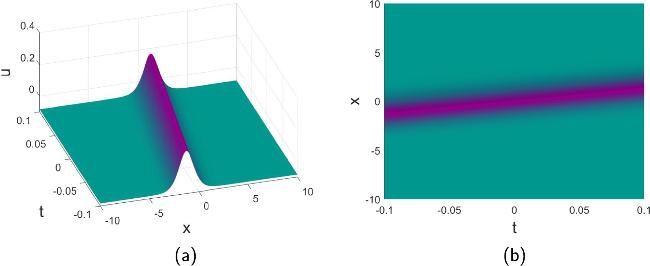
Figure 6. The solitary wave described by equation ( |
In [41], the truncated Painlevé analysis was used to obtain the Cole–Hopf transformation $u=K\frac{{\partial }^{2}}{\partial {x}^{2}}ln(1+{\,\rm{e}\,}^{\theta })$, resulting in solitary solutions with μ = δ(δ + λ)/10 and K = 60/δ or K = 60/(δ + λ). Our new method does not require considering the Painlevé property and the functional inter-dependence of the parameters δ, λ, and μ is directly obtained by solving a system of linear equations. As a result, a different parameter dependence $\mu =-\frac{5{k}^{4}+2c{k}^{2}\delta +c{k}^{2}\lambda }{2{c}^{2}}$ is derived, which gives a new solution (38 ) not mentioned in previous works [39, 41]. The solution yielded by the Cole–Hopf transformation [41] could be obtained by setting c = 0 in our series expansion (35 ). However, in the new solution, c ≠ 0 is required.
In general, equations (37 ) and (38 ) represent different solutions but may coincide by chance at particular parameter values. For example, at δ = 1, λ = 0, $c=-\frac{1}{12}$ and $k=\frac{1}{\sqrt{60}}$, (37 ) and (38 ) can both be rewritten as $u=-\frac{1}{12}(1-\frac{12}{2+2\cosh (\frac{1}{\sqrt{60}}x+\frac{1}{4800\sqrt{15}}t)})$; and at δ = 1, λ = 0, $c=\frac{1}{12}$ and $k=\frac{\pm \,\rm{i}\,}{\sqrt{60}}$ (here, i2 = − 1), both transformed to $u=\frac{1}{12}(1+\frac{12}{-2+2\cos (\frac{1}{\sqrt{60}}x+\frac{1}{4800\sqrt{15}}t)})$.
3.2.2. The two-solitary solution
As before, the search for two-solitary solutions starts from the expansion 37 ), we choose the denominator polynomial
$\begin{eqnarray}u=c+\epsilon (a+b)+{\epsilon }^{2}({p}_{11}{a}^{2}+{p}_{12}{b}^{2}+{p}_{13}ab)+...,\end{eqnarray}$
where $a={C}_{1}{\,\rm{e}\,}^{{\theta }_{1}}$, $b={C}_{2}{\,\rm{e}\,}^{{\theta }_{2}}$, with Ci denoting arbitrary constant, θi = kix + ωit, ${w}_{i}=-({k}_{i}^{5}+c{k}_{1}^{3}\delta +{c}^{2}{k}_{i}\mu )$ for i = 1, 2, and $\begin{eqnarray*}\begin{array}{rcl}{p}_{11} & = & -\frac{{k}_{1}({k}_{1}^{2}(\delta +\lambda )+2c\mu )}{2(16{k}_{1}^{5}+{w}_{1}+4c{k}_{1}^{3}\delta +{c}^{2}{k}_{1}\mu )},\\ {p}_{12} & = & -\frac{{k}_{2}({k}_{2}^{2}(\delta +\lambda )+2c\mu )}{2(16{k}_{2}^{5}+{w}_{2}+4c{k}_{2}^{3}\delta +{c}^{2}{k}_{2}\mu )},\\ {p}_{13} & = & -\frac{({k}_{1}+{k}_{2})({k}_{1}^{2}-{k}_{1}{k}_{2}+{k}_{2}^{2})\delta +{k}_{1}{k}_{2}\lambda +2c\mu }{{({k}_{1}+{k}_{2})}^{5}+({w}_{1}+{w}_{2})+c\delta {({k}_{1}+{k}_{2})}^{3}+{c}^{2}\mu ({k}_{1}+{k}_{2})},\\ & & ....\end{array}\end{eqnarray*}$
Similar to the previous case, by renormalizing the variable a in the one-solitary solution ( $\begin{eqnarray}\begin{array}{rcl}{P}_{2} & = & {b}_{0}+{b}_{1}a+{b}_{2}b+{b}_{3}{a}^{2}+{b}_{4}{b}^{2}+{b}_{5}ab\\ & & +{b}_{6}{a}^{2}b+{b}_{7}a{b}^{2}+{b}_{8}{a}^{2}{b}^{2}+...\end{array}\end{eqnarray}$
where ${\{{b}_{i}\}}_{i=0,1,2,...}$ are undetermined coefficients. By the multiplication and truncation strategy, we obtain the two-soliton solutions in the following two cases.Case1: μ = (δ + λ)δ/10, λ = δ, b0 = 1, ${b}_{1}=\frac{\delta }{15{k}_{1}^{2}}$, ${b}_{2}=\frac{\delta }{15{k}_{2}^{2}}$, ${b}_{3}=\frac{{\delta }^{2}}{900{k}_{1}^{4}}$, ${b}_{4}=\frac{{\delta }^{2}}{900{k}_{2}^{4}}$, and 34 ) is 73 ) of Appendix B.1 .
$\begin{eqnarray*}\begin{array}{rcl}{b}_{5} & = & \frac{{\delta }^{2}(5{k}_{1}^{4}+5{k}_{2}^{4}+3c\delta ({k}_{1}^{2}+{k}_{2}^{2})+20{k}_{1}^{2}{k}_{2}^{2})}{225{k}_{1}^{2}{k}_{2}^{2}{({k}_{1}+{k}_{2})}^{2}(5{k}_{1}^{2}+5{k}_{1}{k}_{2}+5{k}_{2}^{2}+3c\delta )},\\ {b}_{6} & = & \frac{{\delta }^{3}{({k}_{1}-{k}_{2})}^{2}(5{k}_{1}^{2}+5{k}_{2}^{2}-5{k}_{1}^{2}{k}_{2}^{2}+3c\delta )}{13500{k}_{1}^{4}{k}_{2}^{2}{({k}_{1}+{k}_{2})}^{2}(5{k}_{1}^{2}+5{k}_{1}{k}_{2}+5{k}_{2}^{2}+3c\delta )},\\ {b}_{7} & = & \frac{{\delta }^{3}{({k}_{1}-{k}_{2})}^{2}(5{k}_{1}^{2}+5{k}_{2}^{2}-5{k}_{1}^{2}{k}_{2}^{2}+3c\delta )}{13500{k}_{1}^{2}{k}_{2}^{4}{({k}_{1}+{k}_{2})}^{2}(5{k}_{1}^{2}+5{k}_{1}{k}_{2}+5{k}_{2}^{2}+3c\delta )},\\ {b}_{8} & = & \frac{{\delta }^{4}{({k}_{1}-{k}_{2})}^{4}{(5{k}_{1}^{2}+5{k}_{2}^{2}-5{k}_{1}^{2}{k}_{2}^{2}+3c\delta )}^{2}}{810000{k}_{1}^{4}{k}_{2}^{4}{({k}_{1}+{k}_{2})}^{4}{(5{k}_{1}^{2}+5{k}_{1}{k}_{2}+5{k}_{2}^{2}+3c\delta )}^{2}}.\end{array}\end{eqnarray*}$
So, the two-solitary solution of PDE ( $\begin{eqnarray}u=\frac{c+{R}_{1}a+{R}_{2}b+{R}_{3}{a}^{2}+{R}_{4}{b}^{2}+{R}_{5}ab+{R}_{6}{a}^{2}b+{R}_{7}a{b}^{2}+{R}_{8}{a}^{2}{b}^{2}}{1+{b}_{1}a+{b}_{2}b+{b}_{3}{a}^{2}+{b}_{4}{b}^{2}+{b}_{5}ab+{b}_{6}{a}^{2}b+{b}_{7}a{b}^{2}+{b}_{8}{a}^{2}{b}^{2}},\end{eqnarray}$
with $a={C}_{1}{\,\rm{e}\,}^{{k}_{1}x+{\omega }_{1}t}$, $b={C}_{2}{\,\rm{e}\,}^{{k}_{2}x+{\omega }_{2}t}$, where ${\{{C}_{i}\}}_{i=1,2}$ denote arbitrary integral constants, ${\omega }_{i}=-({k}_{i}^{5}+c{k}_{1}^{3}\delta +{c}^{2}{k}_{i}{\delta }^{2}/5)$. The coefficients ${\{{R}_{i}\}}_{i=1,2,...}$ are listed in equation (Case 2: μ = (δ + λ)δ/10, λ = 2δ, b0 = 1, ${b}_{1}=\frac{\delta }{10{k}_{1}^{2}}$, ${b}_{2}=\frac{\delta }{10{k}_{2}^{2}}$, ${b}_{3}=\frac{{\delta }^{2}}{400{k}_{1}^{4}}$, ${b}_{4}=\frac{{\delta }^{2}}{400{k}_{2}^{4}}$, and
$\begin{eqnarray*}\begin{array}{rcl}{b}_{5} & = & \frac{({k}_{1}^{2}+{k}_{2}^{2}){\delta }^{2}}{100{k}_{1}^{2}{k}_{2}^{2}{({k}_{1}+{k}_{2})}^{2}},{b}_{6}=\frac{{({k}_{1}-{k}_{2})}^{2}{\delta }^{3}}{4000{k}_{1}^{4}{k}_{2}^{2}{({k}_{1}+{k}_{2})}^{2}},\\ {b}_{7} & = & \frac{{({k}_{1}-{k}_{2})}^{2}{\delta }^{3}}{4000{k}_{1}^{2}{k}_{2}^{4}{({k}_{1}+{k}_{2})}^{2}},{b}_{8}=\frac{{({k}_{1}-{k}_{2})}^{4}{\delta }^{4}}{160000{k}_{1}^{4}{k}_{2}^{4}{({k}_{1}+{k}_{2})}^{4}}.\end{array}\end{eqnarray*}$
So, the two-solitary solution in this case is $\begin{eqnarray}u=\frac{c+{\tilde{R}}_{1}a+{\tilde{R}}_{2}b+{\tilde{R}}_{3}{a}^{2}+{\tilde{R}}_{4}{b}^{2}+{\tilde{R}}_{5}ab+{\tilde{R}}_{6}{a}^{2}b+{\tilde{R}}_{7}a{b}^{2}+{\tilde{R}}_{8}{a}^{2}{b}^{2}}{1+{b}_{1}a+{b}_{2}b+{b}_{3}{a}^{2}+{b}_{4}{b}^{2}+{b}_{5}ab+{b}_{6}{a}^{2}b+{b}_{7}a{b}^{2}+{b}_{8}{a}^{2}{b}^{2}},\end{eqnarray}$
with $a={C}_{1}{\,\rm{e}\,}^{{k}_{1}x+{\omega }_{1}t}$, $b={C}_{2}{\,\rm{e}\,}^{{k}_{2}x+{\omega }_{2}t}$, where ${\{{C}_{i}\}}_{i=1,2}$ are constants, ${\omega }_{i}=-({k}_{i}^{5}+c{k}_{1}^{3}\delta +3{c}^{2}{k}_{i}{\delta }^{2}/10)$, ${\tilde{R}}_{1}=1+c{b}_{1}$, ${\tilde{R}}_{2}=1+c{b}_{2}$, ${\tilde{R}}_{3}=c{b}_{3}$, ${\tilde{R}}_{4}=c{b}_{4}$, ${\tilde{R}}_{5}=(c+\frac{10{({k}_{1}^{2}-{k}_{2}^{2})}^{2}}{({k}_{1}^{2}+{k}_{2}^{2})\delta }){b}_{5}$, ${\tilde{R}}_{6}=\frac{\delta c+10{k}_{2}^{2}}{\delta }{b}_{6}$, ${\tilde{R}}_{7}=\frac{\delta c+10{k}_{1}^{2}}{\delta }{b}_{7}$, and ${\tilde{R}}_{8}=c{b}_{8}$.In this section, we successfully applied the new approach to search for two-solitary solutions for PDE (34 ). Although the two-solitary type of solution associated with (38 ) does not seem to exist, elliptic type of solutions of this equation could be found, to be detailed next.
3.2.3. The Jacobi elliptic function solution
For the traveling wave, the elliptic function that the origin (34 ) is
$\begin{eqnarray}{u}_{\theta \theta }+{c}_{0}+{c}_{1}u+{c}_{2}{u}^{2}+{c}_{3}{u}^{3}=0,\end{eqnarray}$
where ${\{{c}_{i}\}}_{i=0,1,2,3}$ are undetermined coefficients and θ = kx + ωt. By a substitution and comparison procedure, we get a set of linear algebraic equations for ci, which has a solution in the following two casesCase1: $\mu =\frac{(\delta +\lambda )\delta }{10}$, ${c}_{0}=c+\frac{{c}^{2}(\delta +\lambda )}{10{k}^{2}}$, ${c}_{1}=-(1+\frac{c(\delta +\lambda )}{5{k}^{2}})$, ${c}_{2}=\frac{\delta +\lambda }{10{k}^{2}}$, and c3 = 0, and 45 ) is plotted in figure 7(a).
$\begin{eqnarray}{u}_{\theta \theta }=-c-\frac{{c}^{2}(\delta +\lambda )}{10{k}^{2}}+(1+\frac{c(\delta +\lambda )}{5{k}^{2}})u-\frac{\delta +\lambda }{10{k}^{2}}{u}^{2},\end{eqnarray}$
which has a solution of an exponential type $u\,=\frac{3600c{k}^{4}+120(30{k}^{4}+c{k}^{2}(\delta +\lambda )){\,\rm{e}\,}^{\theta }+c{(\delta +\lambda )}^{2}{\,\rm{e}\,}^{2\theta }}{{((\delta +\lambda ){\,\rm{e}\,}^{\theta }+60{k}^{2})}^{2}}$, or of an elliptic type, i.e., at c = 1 $\begin{eqnarray}u=A{{\rm{cn}}}^{2}(B(kx+\omega t),m),\end{eqnarray}$
where $\omega =-({k}^{5}+c{k}^{3}\delta +\frac{(\delta +\lambda )\delta {c}^{2}k}{10})$, with $\begin{eqnarray*}\begin{array}{rcl}A & = & \frac{-3(\delta +\lambda )-15{k}^{2}+\sqrt{21{(\delta +\lambda )}^{2}+210(\delta +\lambda ){k}^{2}+225{k}^{4}}}{2(\delta +\lambda )},\\ B & = & -\,\rm{i}\,\frac{{(7{(\delta +\lambda )}^{2}+70(\delta +\lambda ){k}^{2}+75{k}^{4})}^{1/4}}{2* \sqrt{5}* {3}^{1/4}},\\ m & = & \frac{-\sqrt{3}(\delta +\lambda )-\sqrt{3}5{k}^{2}+\sqrt{7{(\delta +\lambda )}^{2}+70(\delta +\lambda ){k}^{2}+75{k}^{4}}}{2\sqrt{7{(\delta +\lambda )}^{2}+70(\delta +\lambda ){k}^{2}+75{k}^{4}}}.\end{array}\end{eqnarray*}$
With k = i (here,i2 = − 1), δ = 10, and λ = 5, the solution (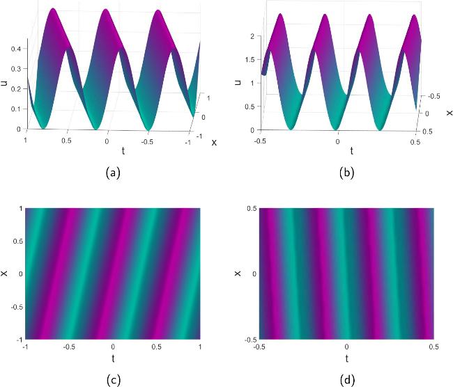
Figure 7. Two elliptic solutions of equation ( |
Case 2: $\mu =-\frac{{k}^{2}(5{k}^{2}+c(2\delta +\lambda ))}{2{c}^{2}}$(c ≠ 0), ${c}_{0}=\frac{c}{2}$, c1 = 0, ${c}_{2}=-\frac{1}{2c}$, c3 = 0, and 47 ) is plotted in figure 7(b).
$\begin{eqnarray}{u}_{\theta \theta }=-\frac{c}{2}+\frac{1}{2c}{u}^{2},\end{eqnarray}$
which has not only exp-type solution $u=c\frac{144{c}^{2}+120c{\rm{e}\,}^{\theta }+{\,\rm{e}}^{2\theta }}{{({\,\rm{e}\,}^{\theta }-12c)}^{2}}$ but also elliptic solutions such as $\begin{eqnarray}u=A{{\rm{sn}}}^{2}(B(kx+\omega t),m),\end{eqnarray}$
where $\omega =-({k}^{5}+c{k}^{3}\delta -\frac{{c}^{2}{k}^{3}(5{k}^{2}+c(2\delta +\lambda ))}{2{c}^{2}})$ with $A=\sqrt{3}c$, B = 0.3779i*k (here, i2 = − 1), m = − 1. At a particular choice c = 1, k = i, δ = 10, and λ = 5, the elliptic solution (It is obvious that equations (45 ) and (47 ) are both periodic behavior with disparate periods and amplitudes, which seems new for equation (34 ) with this parameter dependence as far as we know.
3.3. Application. C: The variable-coefficient modified Kadomatsey–Petviashvilli equation
In this application, the variable-coefficient modified Kadomatsey–Petviashvilli (VCMKP) equation [44] will be considered 49 ) plays a crucial role in many physical problems, such as in fluid dynamics, where it is used to depict the propagation of water waves [46]; or in plasma dynamics and electrodynamics, describing nonlinear ion-acoustic waves [47, 48] and magnetohydrodynamic waves [49]; or in other interesting systems [50, 51]. Recently, the original VCMKP equation (48 ) has also gained more and more attention in physical problems like plasma dynamics, prompting a number of studies [52–55]. In the following, we will compute its one-soliton, two-soliton and elliptic solutions.
$\begin{eqnarray}\begin{array}{l}{u}_{t}+{u}_{xxx}+3{v}_{y}-6{u}^{2}{u}_{x}-6v{u}_{x}\\ \quad +\alpha (t){u}_{y}+\beta (t){u}_{x}=0,\\ {v}_{x}={u}_{y},\end{array}\end{eqnarray}$
where α(t) and β(t) are two functions of time, which becomes [45] $\begin{eqnarray}\begin{array}{l}{u}_{t}+{u}_{xxx}+3{v}_{y}-6{u}^{2}{u}_{x}-6v{u}_{x}=0,\\ {v}_{x}={u}_{y}\end{array}\end{eqnarray}$
at α = 0, β = 0. The MKP equation (3.3.1. The one-soliton solution
With the procedures (8 )-(11 ), we have the following expansion
$\begin{eqnarray}\begin{array}{rcl}u & = & c+a+{p}_{1}{a}^{2}+{p}_{2}{a}^{3}+...,\\ {u}_{t} & = & {\omega }^{{\prime} }(t)(a+2{p}_{1}{a}^{2}+3{p}_{2}{a}^{3}+...),\\ {u}_{xx} & = & {k}^{2}(a+4{p}_{1}{a}^{2}+9{p}_{2}{a}^{3}+...),\end{array}\end{eqnarray}$
where c is an constant, a = Ceθ, θ = kx + ry + ω(t), and $\omega (t)=\int \frac{6{c}^{2}{k}^{2}-{k}^{4}-3{r}^{2}-kr\alpha (\tau )-{k}^{2}\beta (\tau )}{k}\,\rm{d}\,\tau $ with $\begin{eqnarray*}\begin{array}{rcl}{p}_{1} & = & \frac{2ck+r}{{k}^{3}},\\ {p}_{2} & = & \frac{12{c}^{2}{k}^{2}+{k}^{4}+12ckr+3{r}^{2}}{4{k}^{6}},\\ {p}_{3} & = & \frac{8{c}^{3}{k}^{3}+2c{k}^{5}+12{c}^{2}{k}^{2}r+{k}^{4}r+6ck{r}^{2}+{r}^{3}}{2{k}^{9}},\\ & & ....\end{array}\end{eqnarray*}$
The polynomial P1 for the resummation of equation (50 ) is 12 )–(14 ), we obtain a0 = 1, ${a}_{1}=-\frac{2ck+r}{{k}^{3}}$, ${a}_{2}=\frac{4{c}^{2}{k}^{2}-{k}^{4}+4ckr+{r}^{2}}{4{k}^{6}}$, and a3 = 0. Then, the one-soliton solution is 52 ) is transformed into $u=\frac{{k}^{3}r}{2({k}^{4}-{r}^{2})}{{\rm{{\rm{sech}} }}}^{2}(\theta )$. We find that the dispersion expression ω(t) plays a crucial role in the nonlinear analysis, since the variable coefficients α(t) and β(t) determine the envelope velocities along the x- and y-axis. The soliton solution (52 ) have following physical properties: its amplitude is $\frac{{k}^{3}r}{2({k}^{4}-{r}^{2})}$, and the envelop velocities along x-axis and y-axis are $\frac{{k}^{4}+3{r}^{2}+kr\alpha (t)-{k}^{2}\beta (t)}{{k}^{2}}$ and $\frac{{k}^{4}+3{r}^{2}+kr\alpha (t)-{k}^{2}\beta (t)}{kr}$, respectively. That is, when the values of k and r remain constant, varying the coefficients α(t) and β(t) does not change the amplitude of the soliton.
$\begin{eqnarray}{P}_{1}={a}_{0}+{a}_{1}a+{a}_{2}{a}^{2}+{a}_{3}{a}^{3}+...,\end{eqnarray}$
where ${\{{a}_{i}\}}_{i=0,1,2...}$ are undetermined coefficients. Repeating the operations mentioned in equations ( $\begin{eqnarray}u=\frac{4c{k}^{6}+4{k}^{3}({k}^{3}-2{c}^{2}k-cr)a-c({k}^{4}-4{c}^{2}{k}^{2}-4ckr-{r}^{2}){a}^{2}}{4{k}^{6}-4{k}^{3}(2ck+r)a-({k}^{4}-{r}^{2}-4ckr-4{c}^{2}{k}^{2}){a}^{2}}.\end{eqnarray}$
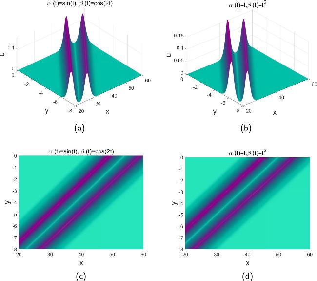
where a = Ceθ, θ = kx + ry + ω(t) and $\omega (t)\,=\int \frac{6{c}^{2}{k}^{2}-{k}^{4}-3{r}^{2}-kr\alpha (\tau )-{k}^{2}\beta (\tau )}{k}\,\rm{d}\,t$. Here, C is an arbitrary integral constant. For convenience, we set c = 0, $C=\frac{2{k}^{3}r}{{k}^{4}-{r}^{2}}$. Then, equation (By taking $\alpha (t)=\sin (t),\beta (t)=\cos (2t)$ or α(t) = t, β(t) = t2, we have different types of solutions which are plotted in figure 8 with c = 0, k = 1, and r = − 4 at t = 1, from which we find that when the time-varying expressions of the variable coefficients α(t) and β(t) are taken to be different, the solution equation (52 ) consistently exhibits a as one-bell-shaped soliton solution. For $r=\frac{\,\rm{i}\,}{\sqrt{3}}{k}^{2}$, $k=\frac{\,\rm{i}\,}{\sqrt{3}}$, and $\alpha (t)=\sin (t),\beta (t)=\cos (2t)$, the one-soliton solution (52 ) can be converted into the trigonometric form equation (53 ) which at at t = 1 are plotted in figure 9 and demonstrates a (x, y)-periodic structure.
$\begin{eqnarray}u=-\frac{1}{1-2\cos \frac{3x-y+(-\cos t+1/2\sin 2t)}{3\sqrt{3}}}.\end{eqnarray}$
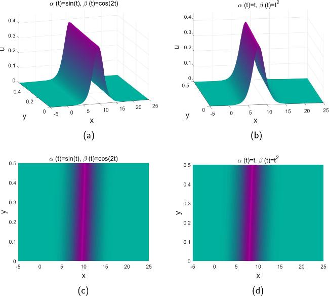
Figure 8. The plots of equation ( |
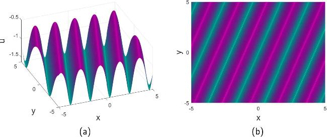
Figure 9. The (x, y)-periodic solution of equation ( |
3.3.2. The two-soliton solution
The expansion for the two-soliton solution is
$\begin{eqnarray}u=c+\epsilon (a+b)+{\epsilon }^{2}({p}_{11}{a}^{2}+{p}_{12}{b}^{2}+{p}_{13}ab)+...,\end{eqnarray}$
where $a={C}_{1}{\,\rm{e}\,}^{{\theta }_{1}}$, $b={C}_{2}{\,\rm{e}\,}^{{\theta }_{2}}$, ${\{{C}_{i}\}}_{i=1,2}$ denote arbitrary integration constants, θi = kix + riy + ωi(t), and ${\omega }_{i}(t)=\int \frac{6{c}^{2}{k}_{i}^{2}-{k}_{i}^{4}-3{r}_{i}^{2}-{k}_{i}{r}_{i}\alpha (\tau )-{k}_{i}^{2}\beta (\tau )}{{k}_{i}}\,\rm{d}\,t$, i = 1, 2, with $\begin{eqnarray*}\begin{array}{rcl}{p}_{11} & = & -\frac{2c{k}_{1}+{r}_{1}}{{k}_{1}^{3}},{p}_{12}=-\frac{2c{k}_{2}+{r}_{2}}{{k}_{2}^{3}},\\ {p}_{13} & = & -\frac{2({k}_{1}+{k}_{2})(2c{k}_{1}{k}_{2}({k}_{1}+{k}_{2})+{k}_{2}^{2}{r}_{1}+{k}_{1}^{2}{r}_{2})}{{k}_{1}^{4}{k}_{2}^{2}+2{k}_{1}^{3}{k}_{2}^{3}-{k}_{2}^{2}{r}_{1}^{2}+2{k}_{1}{k}_{2}{r}_{1}{r}_{2}+{k}_{1}^{2}({k}_{2}^{4}-{r}_{2}^{2})},\\ & & ....\end{array}\end{eqnarray*}$
According to the one-soliton solution (52 ), we set the polynomial for resummation of the series (54 ) to 74 ) of Appendix C.1 . Thus, the two-soliton solution is 75 ) of Appendix C.2 .
$\begin{eqnarray}\begin{array}{rcl}{P}_{2} & = & {b}_{0}+{b}_{1}a+{b}_{2}b+{b}_{3}{a}^{2}+{b}_{4}{b}^{2}+{b}_{5}ab\\ & & +\,{b}_{6}{a}^{2}b+{b}_{7}a{b}^{2}+{b}_{8}{a}^{2}{b}^{2}+...\end{array}\end{eqnarray}$
where ${\{{b}_{i}\}}_{i=0,1,2,...}$ can be computed by the substitution and truncation procedure and are displayed in equation ( $\begin{eqnarray}u=\frac{c+{R}_{1}a+{R}_{2}b+{R}_{3}{a}^{2}+{R}_{4}{b}^{2}+{R}_{5}ab+{R}_{6}{a}^{2}b+{R}_{7}a{b}^{2}+{R}_{8}{a}^{2}{b}^{2}}{1+{b}_{1}a+{b}_{2}b+{b}_{3}{a}^{2}+{b}_{4}{b}^{2}+{b}_{5}ab+{b}_{6}{a}^{2}b+{b}_{7}a{b}^{2}+{b}_{8}{a}^{2}{b}^{2}},\end{eqnarray}$
where $a={C}_{1}{\,\rm{e}\,}^{{\theta }_{1}}$, $b={C}_{2}{\,\rm{e}\,}^{{\theta }_{2}}$ and ${\{{R}_{i}\}}_{i=1,2,\ldots ,8}$ are listed in equation (At c = 0, k1 = 1, k2 = 1.1, r1 = − 4, and r2 = − 4.3, we plot the solution (56 ) with ($\alpha (t)=\sin (t),\beta (t)=\cos (2t)$) and (α(t) = t, β(t) = t2) at t = 1 in figure 10, where the two-bell-shaped soliton equation (56 ) is displayed in figure 10(a)–(c) with ($\alpha (t)=\sin (t),\beta (t)=\cos (2t)$) and in figure 10(b)–(d) with (α(t) = t, β(t) = t2).
Figure 10. The plot of the solution equation ( |
3.3.3. The Jacobi elliptic function solution
In this section, we present the Jacobi elliptic equation solution to the VCMKP equation (48 ), which satisfies the following two equations 48 ) has time-dependent coefficients, we need to separate the equation for variables x and t.
$\begin{eqnarray}{u}_{xx}+{b}_{0}+{b}_{1}u+{b}_{2}{u}^{2}+{b}_{3}{u}^{3}=0,\end{eqnarray}$
$\begin{eqnarray}{u}_{t}^{2}+{c}_{0}+{c}_{1}u+{c}_{2}{u}^{2}+{c}_{3}{u}^{3}+{c}_{4}{u}^{4}=0,\end{eqnarray}$
where ${\{{b}_{i}\}}_{i=0,1,2,3}$ and ${\{{c}_{i}\}}_{i=0,1,\ldots ,4}$ are undetermined coefficients. Usually, we reduce the original PDE to an ODE by introducing η = kx + ωt and considering the traveling wave solution which may lead to an equation f(uηη, u, u2, u3) = 0 as done in previous cases. Now, as the equation (Substituting expansion (50 ) into equations (57 ) and (58 ) and comparing different orders of a, we get a set of linear equations, the solution of which is ${b}_{0}=\frac{c({k}^{3}-4{c}^{2}k-3cr)}{k}$, ${b}_{1}=\frac{6{c}^{2}k-{k}^{3}+6cr}{k}$, ${b}_{2}=-\frac{3r}{k}$, b3 = − 2; and 58 ) is a variable-coefficient ODE.
$\begin{eqnarray*}\begin{array}{rcl}{c}_{0} & = & ({c}^{2}(3{c}^{2}-{k}^{3}+2cr)\frac{{({k}^{4}+3{r}^{2}-6{c}^{2}{k}^{2}+kr\alpha (t)+{k}^{2}\beta (t))}^{2}}{{k}^{5}},\\ {c}_{1} & = & -2c(4{c}^{2}k-{k}^{3}+3cr)\frac{{({k}^{4}+3{r}^{2}-6{c}^{2}{k}^{2}+kr\alpha (t)+{k}^{2}\beta (t))}^{2}}{{k}^{5}},\\ {c}_{2} & = & (6{c}^{2}k-{k}^{3}+6cr)\frac{{({k}^{4}+3{r}^{2}-6{c}^{2}{k}^{2}+kr\alpha (t)+{k}^{2}\beta (t))}^{2}}{{k}^{5}},\\ {c}_{3} & = & -2r\frac{{({k}^{4}+3{r}^{2}-6{c}^{2}{k}^{2}+kr\alpha (t)+{k}^{2}\beta (t))}^{2}}{{k}^{5}},\\ {c}_{4} & = & -\frac{{({k}^{4}+3{r}^{2}-6{c}^{2}{k}^{2}+kr\alpha (t)+{k}^{2}\beta (t))}^{2}}{{k}^{4}}.\end{array}\end{eqnarray*}$
It is obvious that equation (For equation (57 ), there is evidently an exp-function type of solution
$\begin{eqnarray}u=\frac{4c{k}^{6}+4{k}^{3}({k}^{3}-cr-2{c}^{2}k){\,\rm{e}\,}^{kx+\omega (t)}+c(4{c}^{2}{k}^{2}-{k}^{4}+4ckr+{r}^{2}){\,\rm{e}\,}^{2kx+2\omega (t)}}{4{k}^{6}-4{k}^{3}(2ck+r){\,\rm{e}\,}^{kx+\omega (t)}-({k}^{4}-{r}^{2}-4{c}^{2}{k}^{2}-4ckr){\,\rm{e}\,}^{2kx+2\omega (t)}},\end{eqnarray}$
with $\omega =\int \frac{6{c}^{2}{k}^{2}-{k}^{4}-3{r}^{2}-kr\alpha (\tau )-{k}^{2}\beta (\tau )}{k}\,\rm{d}\,t$.Certainly, the exp-function type solution (59 ) also satisfies the elliptic equation (58 ). Since equation (58 ) is a variable-coefficient system, we no longer provide the explicit elliptic function solution for it. Nevertheless, we cannot dismiss the possibility of additional solutions of equation (58 ).
Using the current scheme, we derive soliton and periodic solutions for the VCMKP equation. Alternative solution techniques prevail in the literature including symmetry reduction via Lie group or Lie algebra [44, 52], or conventional approach involving Painlevé analysis, followed by the derivation of Lax pairs and Darboux transformations. In comparison, the new approach here seems much simpler since it does not need all these sophisticated analysis. In addition, unlike many existing methods [13, 14, 16, 17] almost all the parameter dependence is obtained by solving a linear set of equations in the current scheme, which thereby may enable streamlining solution of nonlinear equations.
3.4. Application. D: The Calogero equation
Another interesting equation is the Calogero equation
$\begin{eqnarray}{u}_{t}=3({u}^{2}{u}_{xx}+3u{u}_{x}^{2}+{u}^{4}{u}_{x})+{u}_{xxx},\end{eqnarray}$
which was initially investigated by Calogero and Degasperis [56]. Many authors have studied this equation, [57] revealed that this equation is integrable and can be linearized by means of nonlocal transformation, and it also has a recursion operator capable of generating a hierarchy of evolution equations though its iterative procedure [58]. Here, the one-solitary solution, along with the non-standard elliptic equations of it, will be exhibited through the utilization of the RG scheme.3.4.1. The one-solitary solution
The approximation of equation (60 ) with the simplified RG procedures is 60 ). And ${\{{q}_{i}\}}_{i=1,2,...}$ are the coefficients and they are
$\begin{eqnarray}u=c+\epsilon a+{\epsilon }^{2}{q}_{1}{a}^{2}+{\epsilon }^{3}{q}_{2}{a}^{3}+...,\end{eqnarray}$
where a = ekx+ωt, ω = k3 + 3c2k2 + 3c4k. c is an arbitrary constant solution of PDE ( $\begin{eqnarray*}\begin{array}{rcl}{q}_{1} & = & -\frac{4{c}^{3}+5ck}{2k({c}^{2}+k)},\\ {q}_{2} & = & -\frac{3{c}^{2}+2k+6{c}^{3}{q}_{1}+11ck{q}_{1}}{3{c}^{2}k+4{k}^{2}},\\ & & ....\end{array}\end{eqnarray*}$
With the operations mentioned in the above applications, we cannot derive the exact solitary solution of equation (60 ). That means, the exact solitary solution cannot be expressed as $u=\frac{F}{P}$, where,F, P are the polynomials of different orders of a. Therefore, in order to get the exact solitary solution, we give two polynomials following 63 ) can be simplified as 60 ) in a bilinear form. In fact, the equation (63 ) can be designed as more general form as ${P}_{n}{u}^{n}+{P}_{{n}_{1}}{u}^{n-1}+{P}_{1}u+C=F$(here, ${\{{P}_{i}\}}_{i=1,2,...}$ and F are polynomials) for majority of PDEs. In this system, we have taken n = 2 for convenience.
$\begin{eqnarray}\begin{array}{ll}{P}_{1} & ={a}_{0}+{a}_{1}a+{a}_{2}{a}^{2}+{a}_{3}{a}^{3}+{a}_{4}{a}^{4}+...,\\ {P}_{2} & ={b}_{0}+{b}_{1}a+{b}_{2}{a}^{2}+{b}_{3}{a}^{3}+{b}_{4}{a}^{4}+...,\end{array}\end{eqnarray}$
where ${\{{a}_{i},{b}_{i}\}}_{i=0,1,2...}$ are the undetermined coefficients. Then, we rewrite the solution as $\begin{eqnarray}{P}_{1}{u}^{2}+{P}_{2}u=({b}_{0}c+{a}_{0}{c}^{2})+({b}_{0}+c(2{a}_{0}+{b}_{1}+{a}_{1}c))a+....\end{eqnarray}$
Truncating the polynomial at high order of a in the right side of it(here, we truncate it at the term a6 generally), we can have a0 = 1, ${a}_{1}=\frac{4c}{k}$, ${a}_{2}=\frac{{(2{c}^{2}+k)}^{2}}{{k}^{2}({c}^{2}+k)}$, a3 = 0, a4 = 0, and ${\{{b}_{i}=0\}}_{i=0,1,2,...}$. Then, equation ( $\begin{eqnarray}u=\pm \sqrt{\frac{({c}^{2}+k){(ck+a(2{c}^{2}+k))}^{2}}{{k}^{2}({c}^{2}+k)+4ck({c}^{2}+k)a+{(2{c}^{2}+k)}^{2}{a}^{2}}},\end{eqnarray}$
where a = ekx+ωt, ω = k3 + 3c2k2 + 3c4k. This equation effectively demonstrates the validity of our new approach, as its solution cannot be derived by introducing the transformation $u=\frac{{\partial }^{n}\,{\mathrm{ln}}\,(g)}{\partial {x}^{n}}$ and rewrite equation (3.4.2. The Jacobi elliptic solution
Different from the previous applications mentioned above, the Calogero equation does not conform to the standard elliptic equation f(uηη, u, u2, u3) = 0 depicted in equation (16 ). Nevertheless, we may design a general elliptic equation (65 ) for it 61 ) and its second derivative uθθ = a + 4p2a2 + 9p2a3 + 16p3a4 + . . . into this elliptic equation (65 ) and comparing the different orders of a, the elliptic equation can be rewritten in the following two cases with c = 0 and c ≠ 0, respectively.
$\begin{eqnarray}\begin{array}{rcl}f & = & {c}_{0}+{u}_{\eta \eta }^{2}({c}_{1}+{c}_{2}u+{c}_{3}{u}^{2})\\ & & +{u}_{\eta \eta }({c}_{4}+{c}_{5}u+{c}_{6}{u}^{2})+{u}_{\eta }^{2}({c}_{7}\\ & & +{c}_{8}u+{c}_{9}{u}^{2})+{u}_{\eta }({c}_{10}+{c}_{11}u+{c}_{12}{u}^{2})\\ & & +u({c}_{13}+{c}_{14}u+{c}_{15}{u}^{2}\\ & & +{c}_{16}{u}^{3}+{c}_{17}{u}^{4}+{c}_{18}{u}^{5}+{c}_{19}{u}^{6}+{c}_{20}{u}^{7}+{c}_{21}{u}^{8})\\ & = & 0,\end{array}\end{eqnarray}$
where ${\{{c}_{i}\}}_{i=0,1,2,...}$ are undetermined coefficients. Substituting expansions (Case 1: When c = 0, we have c7 = 1, c14 = − (1 + c5), ${c}_{16}=\frac{2+4{c}_{5}}{k}$, ${c}_{18}=-\frac{1+3{c}_{5}}{{k}^{2}}$, c5 is an arbitrary constant, and the rest of these coefficients are all zero. Then, the elliptic equation (65 ) can be simplified as 66 ) has an exp-type solution $u=\pm \sqrt{\frac{k{\rm{e}\,}^{2\theta }}{k+{\,\rm{e}}^{2\theta }}}$, θ = kx + k3t.
$\begin{eqnarray}{c}_{5}u{u}_{\theta \theta }+{u}_{\eta }^{2}-(1+{c}_{5}){u}^{2}+\frac{2+4{c}_{5}}{k}{u}^{4}-\frac{1+3{c}_{5}}{{k}^{2}}{u}^{6}=0.\end{eqnarray}$
Equation (Case 2: When c = 1, one can get c7 = 1, ${c}_{14}=-\frac{(1+{c}_{5})}{4}$, ${c}_{16}=\frac{1+2{c}_{5}}{2}$, ${c}_{18}=-\frac{1+3{c}_{5}}{4}$, c5 is arbitrary constant, and the rest of these coefficients are all zero. Additionally, the condition k = − 2 is necessary. And
$\begin{eqnarray}{c}_{5}u{u}_{\theta \theta }+{u}_{\theta }^{2}-\frac{(1+{c}_{5})}{4}{u}^{2}+\frac{1+2{c}_{5}}{2}{u}^{4}-\frac{1+3{c}_{5}}{4}{u}^{6}=0.\end{eqnarray}$
This equation also admits a solution $u=\pm \sqrt{\frac{1}{1-2{\,\rm{e}\,}^{\theta }}}$, θ = − 2x − 2t.Since equations (66 ) and (67 ) are not standard elliptic equations, we no longer provide their explicit solutions distinct from the exp-type. However, it must be acknowledged that these equations could still have other solutions.
The one-solitary wave solution and the non-standard elliptic equations that the Calogero equation solution satisfies are derived with the novel method based on the RG scheme in this section. While this equation is not amenable to the traditional Hirota’s bilinear method, our new approach still works. If we take $v={u}^{\frac{1}{{c}_{5}}+1}$, equations (66 ) and (67 ) can be rewritten in the following forms 67 ) can be converted into vθθ − v + 3v2 − 2v3 = 0, which also verifies the transformation v = u2, which is derived in a previous investigation with the truncated Painlevé method [39]. However, in our study, c5 is arbitrary, which signifies that the results (66 ) and (67 ) obtained through the new approach based on the RG scheme are more general.
$\begin{eqnarray}\begin{array}{l}{v}_{\theta \theta }-\frac{{(1+{c}_{5})}^{2}}{{c}_{5}^{2}}v+\frac{(2+4{c}_{5})(1+{c}_{5})}{k{c}_{5}^{2}}{v}^{\frac{2{c}_{5}}{1+{c}_{5}}+1}\\ \quad -\frac{(1+3{c}_{5})(1+{c}_{5})}{k{c}_{5}^{2}}{v}^{\frac{4{c}_{5}}{1+{c}_{5}}+1}=0,\end{array}\end{eqnarray}$
and $\begin{eqnarray}\begin{array}{l}{v}_{\theta \theta }-\frac{{(1+{c}_{5})}^{2}}{4{c}_{5}^{2}}v+\frac{(2+4{c}_{5})(1+{c}_{5})}{4{c}_{5}^{2}}{v}^{\frac{2{c}_{5}}{1+{c}_{5}}+1}\\ \quad -\frac{(1+3{c}_{5})(1+{c}_{5})}{4{c}_{5}^{2}}{v}^{\frac{4{c}_{5}}{1+{c}_{5}}+1}=0.\end{array}\end{eqnarray}$
If we take c5 = 1, the elliptic equation (4. Conclusions
We propose a new polynomial method based on the RG scheme for finding exact solutions of NPDEs in this paper, which yields one- or two-soliton (or multi-soliton, or solitary wave) solutions, periodic solutions (including elliptic function solutions). In this procedure, after a series solution is obtained iteratively, we carry out a resummation to reach a closed expression with a substitution and comparison strategy to get a set of linear algebraic equations that the coefficients of the auxiliary polynomial satisfy. Soliton or solitary wave solutions could be obtained if these algebraic equations are solvable. The form of the auxiliary polynomial for two-soliton (two-solitary wave) solutions could be simplified with the knowledge of the one-soliton (one-solitary wave) solution.
Unlike traditional methods, highly specialized transformations like Cole–Hopf transformation or Darboux transformation are no longer required in the application of our new polynomial method. Our starting point is the perturbative expansion u = c + εu1 + ε2u2 + . . . of the original system, so the Painlevé analysis is not needed, either. With the current approach, new exact solutions are obtained and displayed in Application B and D. We get the same solution as yielded by the Cole–Hopf transformation [41] if we take c = 0 in the perturbative expansion u = c + εu1 + ε2u2 + . . . in Application B. However, if c ≠ 0, a new parameter dependence $\mu =-\frac{5{k}^{4}+2c{k}^{2}\delta +c{k}^{2}\lambda }{2{c}^{2}}$ is obtained, which leads to a new solution. In application D, a reduced equation results from the current analysis that may not pass the Painlevé test.
Nevertheless, the Painlevé analysis could provide interesting information about the functional form of exact solutions, which may be profitably combined with our polynomial method based on the RG scheme. Although most of the time, we only need to solve linear equations in the current computation, if the number of them is large, extra cue may help a lot, like what we have done to obtain multi-soliton solutions. How to obtain these extra cues based on the symmetry, conservation law, singularity structure of the equation under investigation remains a challenge. Furthermore, the resummation scheme presented here seems quite empirical and need to be extended to treat solutions with complex algebraic structures such as lump solutions, rationales of elliptic functions, rogue wave solutions. However, we believe that our new solution scheme will become a viable option for solving NPDEs in the coming future.
Conflict of interest
The authors declare that they have no conflict of interest.
Appendix A The supplements of application A: Hirota–Satsuma–Ito equation
In Appendix A , more details about application A: Hirota–Satsuma–Ito equation will be displayed.
A.1. The details of pij in equation (25 )
$\begin{eqnarray}\begin{array}{rcl}{p}_{11} & = & -\frac{1}{{k}_{1}^{2}},\\ {p}_{12} & = & -\frac{1}{{k}_{2}^{2}},\\ {q}_{21} & = & -\frac{3{p}_{11}}{4{k}_{1}^{2}},\\ {p}_{22} & = & -\frac{3{p}_{12}}{4{k}_{2}^{2}},\\ {h}_{1} & = & 7{k}_{1}^{6}{k}_{2}^{2}+3{k}_{1}^{5}{k}_{2}^{3}+{k}_{2}^{2}{r}_{1}^{2}+{k}_{1}{k}_{2}{r}_{1}({k}_{2}^{3}-2{r}_{2})+{k}_{1}^{4}{k}_{2}(4{k}_{2}^{3}+{r}_{2})\\ & & +{k}_{1}^{3}{k}_{2}^{2}(3{k}_{2}^{3}+2{r}_{1}+3{r}_{2})+{k}_{1}^{2}({k}_{2}^{6}+{r}_{2}^{2}+{k}_{2}^{3}(3{r}_{1}+2{r}_{2}))\\ & & +9{k}_{1}^{2}{k}_{2}^{2}{({k}_{1}+{k}_{2})}^{2}+9c{k}_{1}^{2}{k}_{2}^{2}{({k}_{1}+{k}_{2})}^{2},\\ {p}_{13} & = & -\frac{3{({k}_{1}+{k}_{2})}^{2}(6c{k}_{1}{k}_{2}+{k}_{1}^{3}{k}_{2}+{k}_{2}{r}_{1}+{k}_{1}({k}_{2}^{3}+{r}_{2}))+6{k}_{1}{k}_{2}}{{h}_{1}},\\ & & ....\end{array}\end{eqnarray}$
A.2. The details of ${\{{n}_{i}\}}_{i=1,2,\ldots ,8}$ and ${\{{m}_{i}\}}_{i=1,2,\ldots ,8}$ in equation (27 )
$\begin{eqnarray*}\begin{array}{rcl}{n}_{1} & = & c,\\ {n}_{2} & = & 1+\frac{c}{{k}_{1}^{2}},\\ {n}_{3} & = & 1+\frac{c}{{k}_{2}^{2}},\\ {n}_{4} & = & \frac{c}{4{k}_{1}^{4}},\\ {n}_{5} & = & \frac{c}{4{k}_{2}^{4}},\\ num\_{n}_{6} & = & {k}_{2}^{2}({k}_{1}^{2}(9{c}^{2}({k}_{1}^{2}+{k}_{2}^{2})+({k}_{1}^{2}+{k}_{2}^{2})\\ & & \times {({k}_{1}^{2}-{k}_{2}^{2})}^{2}+2c(5{k}_{1}^{4}-7{k}_{1}^{2}{k}_{2}^{2}+5{k}_{2}^{4}))\\ & & +{k}_{1}(2{k}_{1}^{2}(c+{k}_{1}^{2})+(c-3{k}_{1}^{2}){k}_{2}^{2}+{k}_{2}^{4}){r}_{1}+{r}_{1}^{2}\\ & & \times (c+{k}_{1}^{2}+{k}_{2}^{2}))+{k}_{1}{k}_{2}({k}_{1}^{5}-3{k}_{1}^{3}{k}_{2}^{2}\\ & & +2{k}_{1}{k}_{2}^{4}+c{k}_{1}({k}_{1}^{2}+{k}_{2}^{2})-2(c+{k}_{1}^{2}+{k}_{2}^{2}){r}_{1}){r}_{2}\\ & & +{k}_{1}^{2}(c+{k}_{1}^{2}+{k}_{2}^{2}){r}_{2}^{2},\\ den\_{n}_{6} & = & {k}_{1}^{2}{k}_{2}^{2}({k}_{2}^{2}({k}_{1}^{2}{({k}_{1}+{k}_{2})}^{2}(9c+{k}_{1}^{2}\\ & & +{k}_{1}{k}_{2}+{k}_{2}^{2})+{k}_{1}({k}_{1}+{k}_{2})(2{k}_{1}+{k}_{2}){r}_{1}\\ & & +{r}_{1}^{2})+{k}_{1}{k}_{2}({k}_{1}({k}_{1}+{k}_{2})({k}_{1}+2{k}_{2})-2{r}_{1}){r}_{2}+{k}_{1}^{2}{r}_{2}^{2}),\\ num\_{n}_{7} & = & (c+{k}_{2}^{2})({k}_{2}^{2}({k}_{1}^{2}{({k}_{1}-{k}_{2})}^{2}\\ & & \times (9c+{k}_{1}^{2}-{k}_{1}{k}_{2}+{k}_{2}^{2})+{k}_{1}(2{k}_{1}^{2}-3{k}_{1}{k}_{2}+{k}_{2}^{2}){r}_{1}\\ & & +{r}_{1}^{2})+{k}_{1}{k}_{2}({k}_{1}({k}_{1}-2{k}_{2}({k}_{1}-{k}_{2})-2{r}_{1}){r}_{2}+{k}_{1}^{2}{r}_{2}^{2}),\\ den\_{n}_{7} & = & 4{k}_{1}^{4}{k}_{2}^{2}({k}_{2}^{2}({k}_{1}^{2}{({k}_{1}+{k}_{2})}^{2}\\ & & \times (9c+{k}_{1}^{2}+{k}_{1}{k}_{2}+{k}_{2}^{2})+({k}_{1}^{2}+{k}_{1}{k}_{2})(2{k}_{1}+{k}_{2}){r}_{1}\\ & & +{r}_{1}^{2})+{k}_{1}{k}_{2}({k}_{1}^{2}+{k}_{1}{k}_{2})({k}_{1}+2{k}_{2})-2{r}_{1}){r}_{2}+{k}_{1}^{2}{r}_{2}^{2}),\\ num\_{n}_{8} & = & (c+{k}_{1}^{2})({k}_{2}^{2}({k}_{1}^{2}{({k}_{1}-{k}_{2})}^{2}\end{array}\end{eqnarray*}$
$\begin{eqnarray}\begin{array}{rcl} & & \times (9c+{k}_{1}^{2}-{k}_{1}{k}_{2}+{k}_{2}^{2})+{k}_{1}(2{k}_{1}^{2}-3{k}_{1}{k}_{2}+{k}_{2}^{2}){r}_{1}\\ & & +{r}_{1}^{2})+{k}_{1}{k}_{2}({k}_{1}({k}_{1}-2{k}_{2}({k}_{1}-{k}_{2})-2{r}_{1}){r}_{2}+{k}_{1}^{2}{r}_{2}^{2}),\\ den\_{n}_{8} & = & 4{k}_{2}^{4}{k}_{1}^{2}({k}_{2}^{2}({k}_{1}^{2}{({k}_{1}+{k}_{2})}^{2}\\ & & \times (9c+{k}_{1}^{2}+{k}_{1}{k}_{2}+{k}_{2}^{2})+({k}_{1}^{2}+{k}_{1}{k}_{2})(2{k}_{1}+{k}_{2}){r}_{1}\\ & & +{r}_{1}^{2})+{k}_{1}{k}_{2}({k}_{1}^{2}+{k}_{1}{k}_{2})({k}_{1}+2{k}_{2})-2{r}_{1}){r}_{2}+{k}_{1}^{2}{r}_{2}^{2}),\\ mum\_{n}_{9} & = & ({k}_{1}^{6}{k}_{2}^{2}-3{k}_{1}^{5}{k}_{2}^{3}+{k}_{2}^{2}{r}_{1}^{2}\\ & & +{k}_{1}^{3}{k}_{2}^{2}(2{r}_{1}-3{r}_{2}-3{k}_{2}^{3})+{k}_{1}{k}_{2}{r}_{1}({k}_{2}^{3}-2{r}_{2})\\ & & +{k}_{1}^{4}{k}_{2}(4{k}_{2}^{3}+{r}_{2})+{k}_{1}^{2}({k}_{2}^{6}+{r}_{2}^{2}+{k}_{2}^{3}\\ & & \times (3{r}_{1}+2{r}_{2})+9c{k}_{1}^{2}{k}_{2}^{2}{({k}_{1}-{k}_{2})}^{2}{)}^{2},\\ den\_{n}_{9} & = & 16{k}_{1}^{4}{k}_{2}^{4}({k}_{1}^{6}{k}_{2}^{2}+3{k}_{1}^{5}{k}_{2}^{3}+{k}_{2}^{2}{r}_{1}^{2}\\ & & +{k}_{1}{k}_{2}{r}_{1}({k}_{2}^{3}-2{r}_{2})+{k}_{1}^{4}{k}_{2}(4{k}_{2}^{3}+{r}_{2})\\ & & {k}_{1}^{3}{k}_{2}^{2}(3{k}_{2}^{3}+2{r}_{1}+3{r}_{2})+{k}_{1}^{2}({k}_{2}^{6}+{r}_{2}^{2}+{k}_{2}^{3}\\ & & \times (3{r}_{1}+2{r}_{2}))+9c{k}_{1}^{2}{k}_{2}^{2}{({k}_{1}+k2)}^{2}{)}^{2},\\ {n}_{6} & = & \frac{num\rm{\_}\,{n}_{6}}{den\rm{\_}{n}_{6}},{n}_{7}=\frac{num\rm{\_}{n}_{7}}{den\,\rm{\_}{n}_{7}},\\ {n}_{8} & = & \frac{num\rm{\_}\,{n}_{8}}{den\rm{\_}{n}_{8}},{n}_{9}=\frac{num\rm{\_}{n}_{9}}{den\,\rm{\_}{n}_{9}}.\end{array}\end{eqnarray}$
And $\begin{eqnarray*}\begin{array}{rcl}{m}_{1} & = & \frac{1}{{k}_{1}^{2}},\\ {m}_{2} & = & \frac{1}{{k}_{2}^{2}},\\ {m}_{3} & = & \frac{1}{4{k}_{1}^{4}},\\ {m}_{4} & = & \frac{1}{4{k}_{2}^{4}},\\ num\_{m}_{5} & = & {k}_{1}^{6}{k}_{2}^{2}+2{k}_{1}^{3}{k}_{2}^{2}{r}_{1}+{k}_{2}^{2}{r}_{1}^{2}\\ & & +{k}_{1}{k}_{2}{r}_{1}({k}_{2}^{3}-2{r}_{2})+{k}_{1}^{2}{({k}_{2}^{3}+{r}_{2})}^{2}\\ & & +{k}_{1}^{4}{k}_{2}(4{k}_{2}^{3}+{r}_{2})+9c{k}_{1}^{2}{k}_{2}^{2}({k}_{1}^{2}+{k}_{2}^{2}),\\ den\_{m}_{5} & = & {k}_{1}^{2}{k}_{2}^{2}({k}_{1}^{6}{k}_{2}^{2}+3{k}_{1}^{5}{k}_{2}^{3}+{k}_{2}^{2}{r}_{1}^{2}\\ & & +{k}_{1}{k}_{2}{r}_{1}({k}_{2}^{3}-2{r}_{2})+{k}_{1}^{4}{k}_{2}(4{k}_{2}^{3}+{r}_{2})\\ & & +{k}_{1}^{3}{k}_{2}^{2}(3{k}_{2}^{3}+2{r}_{1}+3{r}_{2})+{k}_{1}^{2}({k}_{2}^{6}+{r}_{2}^{2}\\ & & +{k}_{2}^{3}(3{r}_{1}+2{r}_{2})+9c{k}_{1}^{2}{k}_{2}^{2}{({k}_{1}+{k}_{2})}^{2}),\\ num\_{m}_{6} & = & {k}_{1}^{6}{k}_{2}^{2}-3{k}_{1}^{5}{k}_{2}^{3}+{k}_{2}^{2}{r}_{1}^{2}+{k}_{1}^{3}{k}_{2}\\ & & \times (2{r}_{1}-3{r}_{2}-3{k}_{2}^{3})+{k}_{1}{k}_{2}{r}_{1}({k}_{2}^{3}-2{r}_{2})\\ & & +{k}_{1}^{4}{k}_{2}(4{k}_{2}^{3}+{r}_{2})+{k}_{1}^{2}({k}_{2}^{6}+{r}_{2}^{2}\\ & & +{k}_{2}^{3}(2{r}_{2}-3{r}_{1}))+9c{k}_{1}^{2}{k}_{2}^{2}{({k}_{1}-{k}_{2})}^{2},\\ den\_{m}_{6} & = & 4{k}_{1}^{4}{k}_{2}^{2}({k}_{1}^{6}{k}_{2}^{2}+3{k}_{1}^{5}{k}_{2}^{3}+{k}_{2}^{2}{r}_{1}^{2}\\ & & +9c{k}_{1}^{2}{k}_{2}^{2}{({k}_{1}+{k}_{2})}^{2}+{k}_{1}{k}_{2}{r}_{1}({k}_{2}^{3}-2{r}_{2})\\ & & +{k}_{1}^{4}{k}_{2}(4{k}_{2}^{3}+{r}_{2})+{k}_{1}^{3}{k}_{2}^{2}(3{k}_{2}^{3}+2{r}_{1}+3{r}_{2})\\ & & +\,{k}_{1}^{2}({k}_{2}^{6}+{r}_{2}^{2}+{k}_{2}^{3}(3{r}_{1}+2{r}_{2}))),\\ num\_{m}_{7} & = & {k}_{1}^{6}{k}_{2}^{2}-3{k}_{1}^{5}{k}_{2}^{3}+{k}_{2}^{2}{r}_{1}^{2}\\ & & +{k}_{1}^{3}{k}_{2}(2{r}_{1}-3{r}_{2}-3{k}_{2}^{3})+{k}_{1}{k}_{2}{r}_{1}({k}_{2}^{3}-2{r}_{2})\\ & & +{k}_{1}^{4}{k}_{2}(4{k}_{2}^{3}+{r}_{2})+{k}_{1}^{2}({k}_{2}^{6}+{r}_{2}^{2}\\ & & +{k}_{2}^{3}(2{r}_{2}-3{r}_{1}))+9c{k}_{1}^{2}{k}_{2}^{2}{({k}_{1}-{k}_{2})}^{2},\end{array}\end{eqnarray*}$
$\begin{eqnarray}\begin{array}{rcl}den\_{m}_{7} & = & 4{k}_{2}^{4}{k}_{1}^{2}({k}_{1}^{6}{k}_{2}^{2}+3{k}_{1}^{5}{k}_{2}^{3}\\ & & +{k}_{2}^{2}{r}_{1}^{2}+9c{k}_{1}^{2}{k}_{2}^{2}{({k}_{1}+{k}_{2})}^{2}+{k}_{1}{k}_{2}{r}_{1}({k}_{2}^{3}-2{r}_{2})\\ & & +{k}_{1}^{4}{k}_{2}(4{k}_{2}^{3}+{r}_{2})+{k}_{1}^{3}{k}_{2}^{2}(3{k}_{2}^{3}+2{r}_{1}\\ & & +3{r}_{2})+{k}_{1}^{2}({k}_{2}^{6}+{r}_{2}^{2}+{k}_{2}^{3}(3{r}_{1}+2{r}_{2}))),\\ mum\_{m}_{8} & = & ({k}_{1}^{6}{k}_{2}^{2}-3{k}_{1}^{5}{k}_{2}^{3}+{k}_{2}^{2}{r}_{1}^{2}\\ & & +{k}_{1}^{3}{k}_{2}^{2}(2{r}_{1}-3{r}_{2}-3{k}_{2}^{3})+{k}_{1}{k}_{2}{r}_{1}({k}_{2}^{3}-2{r}_{2})\\ & & +{k}_{1}^{4}{k}_{2}(4{k}_{2}^{3}+{r}_{2})+{k}_{1}^{2}({k}_{2}^{6}+{r}_{2}^{2}\\ & & +{k}_{2}^{3}(3{r}_{1}+2{r}_{2})+9c{k}_{1}^{2}{k}_{2}^{2}{({k}_{1}-{k}_{2})}^{2}{)}^{2},\\ den\_{m}_{8} & = & 16{k}_{1}^{4}{k}_{2}^{4}({k}_{1}^{6}{k}_{2}^{2}+3{k}_{1}^{5}{k}_{2}^{3}\\ & & +{k}_{2}^{2}{r}_{1}^{2}+{k}_{1}{k}_{2}{r}_{1}({k}_{2}^{3}-2{r}_{2})+{k}_{1}^{4}{k}_{2}(4{k}_{2}^{3}+{r}_{2})\\ & & {k}_{1}^{3}{k}_{2}^{2}(3{k}_{2}^{3}+2{r}_{1}+3{r}_{2})+{k}_{1}^{2}({k}_{2}^{6}+{r}_{2}^{2}\\ & & +{k}_{2}^{3}(3{r}_{1}+2{r}_{2}))+9c{k}_{1}^{2}{k}_{2}^{2}{({k}_{1}+k2)}^{2}{)}^{2},\\ {m}_{5} & = & \frac{num\rm{\_}\,{m}_{5}}{den\rm{\_}{m}_{5}},{m}_{6}=\frac{num\rm{\_}{m}_{6}}{den\,\rm{\_}{m}_{6}},\\ {m}_{7} & = & \frac{num\rm{\_}\,{m}_{7}}{den\rm{\_}{m}_{7}},{m}_{8}=\frac{num\rm{\_}{m}_{8}}{den\,\rm{\_}{m}_{8}}.\end{array}\end{eqnarray}$
Appendix B The supplements of application B: The general class of 5th-order evolution equation
In appendix B, more details about Application B: The General Class of 5th-Order Evolution equation will be shown.
B.1. The details of the Ri in the equation (41 )
$\begin{eqnarray}\begin{array}{rcl}{R}_{1} & = & 1+\frac{c\delta }{15{k}_{1}^{2}},\\ {R}_{2} & = & 1+\frac{c\delta }{15{k}_{2}^{2}},\\ {R}_{3} & = & \frac{c{\delta }^{2}}{900{k}_{1}^{4}},\\ {R}_{4} & = & \frac{c{\delta }^{2}}{900{k}_{2}^{4}},\\ {R}_{5} & = & \frac{\delta (75{({k}_{1}^{2}-{k}_{2}^{2})}^{2}({k}_{1}^{2}+{k}_{2}^{2})+10c(5{k}_{1}^{4}+5{k}_{2}^{4}-7{k}_{1}^{2}{k}_{2}^{2})\delta +3{c}^{2}({k}_{1}^{2}2+{k}_{2}^{2}){\delta }^{2})}{225{k}_{1}^{2}{k}_{2}^{2}{({k}_{1}+{k}_{2})}^{2}(5{k}_{1}^{2}+5{k}_{1}{k}_{2}+5{k}_{2}^{2}+3c\delta )},\\ {R}_{6} & = & \frac{{({k}_{1}-{k}_{2})}^{2}{\delta }^{2}(15{k}_{2}^{2}+c\delta )(5{k}_{1}^{2}+5{k}_{2}^{2}-5{k}_{1}^{2}{k}_{2}^{2}+3c\delta )}{13500{k}_{1}^{4}{k}_{2}^{2}{({k}_{1}+{k}_{2})}^{2}(5{k}_{1}^{2}+5{k}_{1}{k}_{2}+5{k}_{2}^{2}+3c\delta )},\\ {R}_{7} & = & \frac{{({k}_{1}-{k}_{2})}^{2}{\delta }^{2}(15{k}_{1}^{2}+c\delta )(5{k}_{1}^{2}+5{k}_{2}^{2}-5{k}_{1}^{2}{k}_{2}^{2}+3c\delta )}{13500{k}_{1}^{2}{k}_{2}^{4}{({k}_{1}+{k}_{2})}^{2}(5{k}_{1}^{2}+5{k}_{1}{k}_{2}+5{k}_{2}^{2}+3c\delta )},\\ {R}_{8} & = & \frac{c{({k}_{1}-{k}_{2})}^{4}{\delta }^{4}{(5{k}_{1}^{2}+5{k}_{2}^{2}-5{k}_{1}^{2}{k}_{2}^{2}+3c\delta )}^{2}}{810000{k}_{1}^{4}{k}_{2}^{4}{({k}_{1}+{k}_{2})}^{4}{(5{k}_{1}^{2}+5{k}_{1}{k}_{2}+5{k}_{2}^{2}+3c\delta )}^{2}},\end{array}\end{eqnarray}$
Appendix C The supplements of application C: The variable-coefficient modified kadomatsey–petviashvilli equation
In this Appendix, more details about Application C:The Variable-Coefficient Modified Kadomatsey–Petviashvilli equation will be listed.
C.1. The Details of the ${\{{b}_{i}\}}_{i=1,2,\ldots ,}$ in Equation (55 )
$\begin{eqnarray}\begin{array}{rcl}{b}_{0} & = & 1,\\ {b}_{1} & = & -\frac{2c{k}_{1}+{r}_{1}}{{k}_{1}^{3}},\\ {b}_{2} & = & -\frac{2c{k}_{2}+{r}_{2}}{{k}_{2}^{3}},\\ {b}_{3} & = & \frac{4{c}^{2}{k}_{1}^{2}-{k}_{1}^{4}+4c{k}_{1}{r}_{1}+{r}_{1}^{2}}{4{k}_{1}^{6}},\\ {b}_{4} & = & \frac{4{c}^{2}{k}_{2}^{2}-{k}_{2}^{4}+4c{k}_{2}{r}_{2}+{r}_{2}^{2}}{4{k}_{2}^{6}},\\ num\_{b}_{5} & = & 2{k}_{2}^{3}(-{k}_{1}^{5}{k}_{2}^{2}+c{r}_{1}({k}_{1}^{4}+{k}_{1}^{2}{k}_{2}^{2}-{r}_{1}^{2})+2{c}^{2}({k}_{1}^{5}+{k}_{1}^{3}{k}_{2}^{2}-{k}_{1}{r}_{1}^{2}))\\ & & +{k}_{2}^{2}(2c{k}_{1}+{r}_{1})({k}_{1}^{4}+{k}_{1}^{2}{k}_{2}^{2}+4c{k}_{1}{r}_{1}-{r}_{1}^{2}){r}_{2}-2{k}_{1}{k}_{2}(c{k}_{1}-{r}_{1})(2c{k}_{1}+{r}_{1}){r}_{2}^{2}\\ & & -{k}_{1}^{2}(2c{k}_{1}+{r}_{1}){r}_{2}^{3},\\ {b}_{5} & = & \frac{num\_{b}_{5}}{{k}_{1}^{3}{k}_{2}^{3}({k}_{2}({k}_{1}({k}_{1}+{k}_{2})+{r}_{1})-{k}_{1}{r}_{2})({k}_{1}{k}_{2}({k}_{1}+{k}_{2})-{k}_{2}{r}_{1}+{k}_{1}{r}_{2})},\\ {b}_{6} & = & -\frac{(2c{k}_{1}-{k}_{1}^{2}+{r}_{1})(2c{k}_{1}+{k}_{1}^{2}+{r}_{1})(2c{k}_{2}+{r}_{2})(-{k}_{2}({k}_{1}({k}_{2}-{k}_{1})+{r}_{1})+{k}_{1}{r}_{2})({k}_{1}^{2}{k}_{2}+{k}_{2}{r}_{1}-{k}_{1}({k}_{2}^{2}+{r}_{2}))}{4{k}_{1}^{6}{k}_{2}^{3}({k}_{2}({k}_{1}({k}_{1}+{k}_{2})+{r}_{1})-{k}_{1}{r}_{2})({k}_{1}{k}_{2}({k}_{1}+{k}_{2})-{k}_{2}{r}_{1}+{k}_{1}{r}_{2})},\\ {b}_{7} & = & -\frac{(2c{k}_{2}-{k}_{2}^{2}+{r}_{2})(2c{k}_{2}+{k}_{2}^{2}+{r}_{2})(2c{k}_{1}+{r}_{1})(-{k}_{2}({k}_{1}({k}_{2}-{k}_{1})+{r}_{1})+{k}_{1}{r}_{2})({k}_{1}^{2}{k}_{2}+{k}_{2}{r}_{1}-{k}_{1}({k}_{2}^{2}+{r}_{2}))}{4{k}_{1}^{3}{k}_{2}^{6}({k}_{2}({k}_{1}({k}_{1}+{k}_{2})+{r}_{1})-{k}_{1}{r}_{2})({k}_{1}{k}_{2}({k}_{1}+{k}_{2})-{k}_{2}{r}_{1}+{k}_{1}{r}_{2})},\\ {b}_{8} & = & \frac{(2c{k}_{1}-{k}_{1}^{2}+{r}_{1})(2c{k}_{1}+{k}_{1}^{2}+{r}_{1})(2c{k}_{2}-{k}_{2}^{2}+{r}_{2})(2c{k}_{2}+{k}_{2}^{2}+{r}_{2}){({k}_{2}({k}_{1}({k}_{2}-{k}_{1})+{r}_{1})-{k}_{1}{r}_{2})}^{2}{({k}_{1}^{2}{k}_{2}+{k}_{2}{r}_{1}-{k}_{1}({k}_{2}^{2}+{r}_{2}))}^{2}}{16{k}_{1}^{6}{k}_{2}^{6}{({k}_{2}({k}_{1}({k}_{1}+{k}_{2})+{r}_{1})-{k}_{1}{r}_{2})}^{2}{({k}_{1}{k}_{2}({k}_{1}+{k}_{2})-{k}_{2}{r}_{1}+{k}_{1}{r}_{2})}^{2}}.\end{array}\end{eqnarray}$
C.2. The Details of ${\{{R}_{i}\}}_{i=1,2,\ldots ,}$ in Equation (56 )
$\begin{eqnarray}\begin{array}{rcl}{R}_{1} & = & 1-\frac{c(2c{k}_{1}+{r}_{1})}{{k}_{1}^{3}},\\ {R}_{2} & = & 1-\frac{c(2c{k}_{2}+{r}_{2})}{{k}_{2}^{3}},\\ {R}_{3} & = & \frac{c(4{c}^{2}{k}_{1}^{2}-{k}_{1}^{4}+4c{k}_{1}{r}_{1}+{r}_{1}^{2})}{4{k}_{1}^{6}},\\ {R}_{4} & = & \frac{c(4{c}^{2}{k}_{2}^{2}-{k}_{2}^{4}+4c{k}_{2}{r}_{2}+{r}_{2}^{2})}{4{k}_{2}^{6}},\\ num\_{R}_{5} & = & c(2{k}_{2}^{3}(-{k}_{1}^{5}{k}_{2}^{2}+c{r}_{1}({k}_{1}^{4}+{k}_{1}^{2}{k}_{2}^{2}-{r}_{1}^{2})+2{c}^{2}({k}_{1}^{5}+{k}_{1}^{3}{k}_{2}^{2}-{k}_{1}{r}_{1}^{2}))\\ & & +{k}_{2}^{2}(2c{k}_{1}+{r}_{1})({k}_{1}^{4}+{k}_{1}^{2}{k}_{2}^{2}+4c{k}_{1}{r}_{1}-{r}_{1}^{2}){r}_{2})-2{k}_{1}{k}_{2}(c{k}_{1}-{r}_{1})(2c{k}_{1}+{r}_{1}){r}_{2}^{2}-{k}_{1}^{2}(2c{k}_{1}+{r}_{1}){r}_{2}^{3}),\\ {R}_{5} & = & -\frac{2c{k}_{1}+{r}_{1}}{{k}_{1}^{3}}-\frac{2c{k}_{2}+{r}_{2}}{{k}_{2}^{3}}+\frac{num\_{R}_{5}}{{k}_{1}^{3}{k}_{2}^{3}({k}_{2}({k}_{1}({k}_{1}+{k}_{2})+{r}_{1})-{k}_{1}{r}_{2})({k}_{1}{k}_{2}({k}_{1}+{k}_{2})-{k}_{2}{r}_{1}+{k}_{1}{r}_{2})}\\ & & +\frac{2({k}_{1}+{k}_{2})(2c{k}_{1}{k}_{2}({k}_{1}+{k}_{2})+{k}_{2}^{2}{r}_{1}+{k}_{1}^{2}{r}_{2})}{{k}_{1}^{4}{k}_{2}^{2}+2{k}_{1}^{3}{k}_{2}^{3}-{k}_{2}^{2}{r}_{1}+2{k}_{1}{k}_{2}{r}_{1}{r}_{2}+{k}_{1}^{2}({k}_{2}^{4}-{r}_{2}^{2})},\\ {R}_{6} & = & -\frac{(4{c}^{2}{k}_{1}^{2}-{k}_{1}^{4}+4c{k}_{1}{r}_{1}+{r}_{1}^{2})(2{c}^{2}{k}_{2}-{k}_{2}^{3}+c{r}_{2})({k}_{1}^{4}{k}_{2}^{2}-2{k}_{1}^{3}{k}_{2}^{3}-{k}_{2}^{2}{r}_{1}^{2}+2{k}_{1}{k}_{2}{r}_{1}{r}_{2}+{k}_{1}^{2}({k}_{2}^{4}-{r}_{2}^{2}))}{4{k}_{1}^{6}{k}_{2}^{3}({k}_{2}({k}_{1}({k}_{1}+{k}_{2})+{r}_{1})-{k}_{1}{r}_{2})({k}_{1}{k}_{2}({k}_{1}+{k}_{2})-{k}_{2}{r}_{1}+{k}_{1}{r}_{2})},\\ {R}_{7} & = & -\frac{(4{c}^{2}{k}_{2}^{2}-{k}_{2}^{4}+4c{k}_{2}{r}_{2}+{r}_{2}^{2})(2{c}^{2}{k}_{1}-{k}_{1}^{3}+c{r}_{1})({k}_{1}^{4}{k}_{2}^{2}-2{k}_{1}^{3}{k}_{2}^{3}-{k}_{2}^{2}{r}_{1}^{2}+2{k}_{1}{k}_{2}{r}_{1}{r}_{2}+{k}_{1}^{2}({k}_{2}^{4}-{r}_{2}^{2}))}{4{k}_{1}^{3}{k}_{2}^{6}({k}_{2}({k}_{1}({k}_{1}+{k}_{2})+{r}_{1})-{k}_{1}{r}_{2})({k}_{1}{k}_{2}({k}_{1}+{k}_{2})-{k}_{2}{r}_{1}+{k}_{1}{r}_{2})},\\ {R}_{8} & = & \frac{c(4{c}^{2}{k}_{1}^{2}-{k}_{1}^{4}+4c{k}_{1}{r}_{1}+{r}_{1}^{2})(4{c}^{2}{k}_{2}^{2}-{k}_{2}^{4}+4c{k}_{2}{r}_{2}+{r}_{2}^{2}){({k}_{1}^{4}{k}_{2}^{2}-2{k}_{1}^{3}{k}_{2}^{3}-{k}_{2}^{2}{r}_{1}^{2}+2{k}_{1}{k}_{2}{r}_{1}{r}_{2}+{k}_{1}^{2}({k}_{2}^{4}-{r}_{2}^{2}))}^{2}}{16{k}_{1}^{6}{k}_{2}^{6}{({k}_{2}({k}_{1}({k}_{1}+{k}_{2})+{r}_{1})-{k}_{1}{r}_{2})}^{2}{({k}_{1}{k}_{2}({k}_{1}+{k}_{2})-{k}_{2}{r}_{1}+{k}_{1}{r}_{2})}^{2}}.\end{array}\end{eqnarray}$